
Unusual Fish Assemblages Associated with Environmental Changes in the East China Sea in February and March 2017


Abstract
1. Introduction
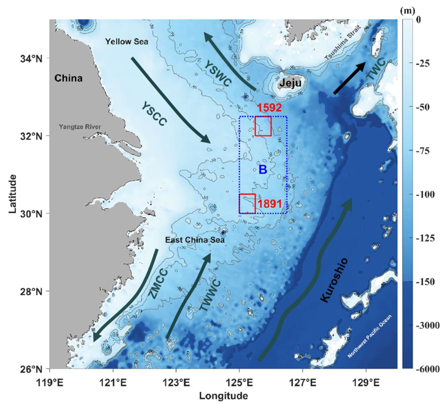
2. Materials and Methods
2.1. Satellite Data and Processing
2.2. Temperature and Geostrophic Currents from ARMOR3D
3. Results
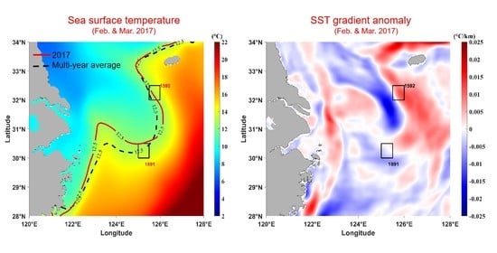
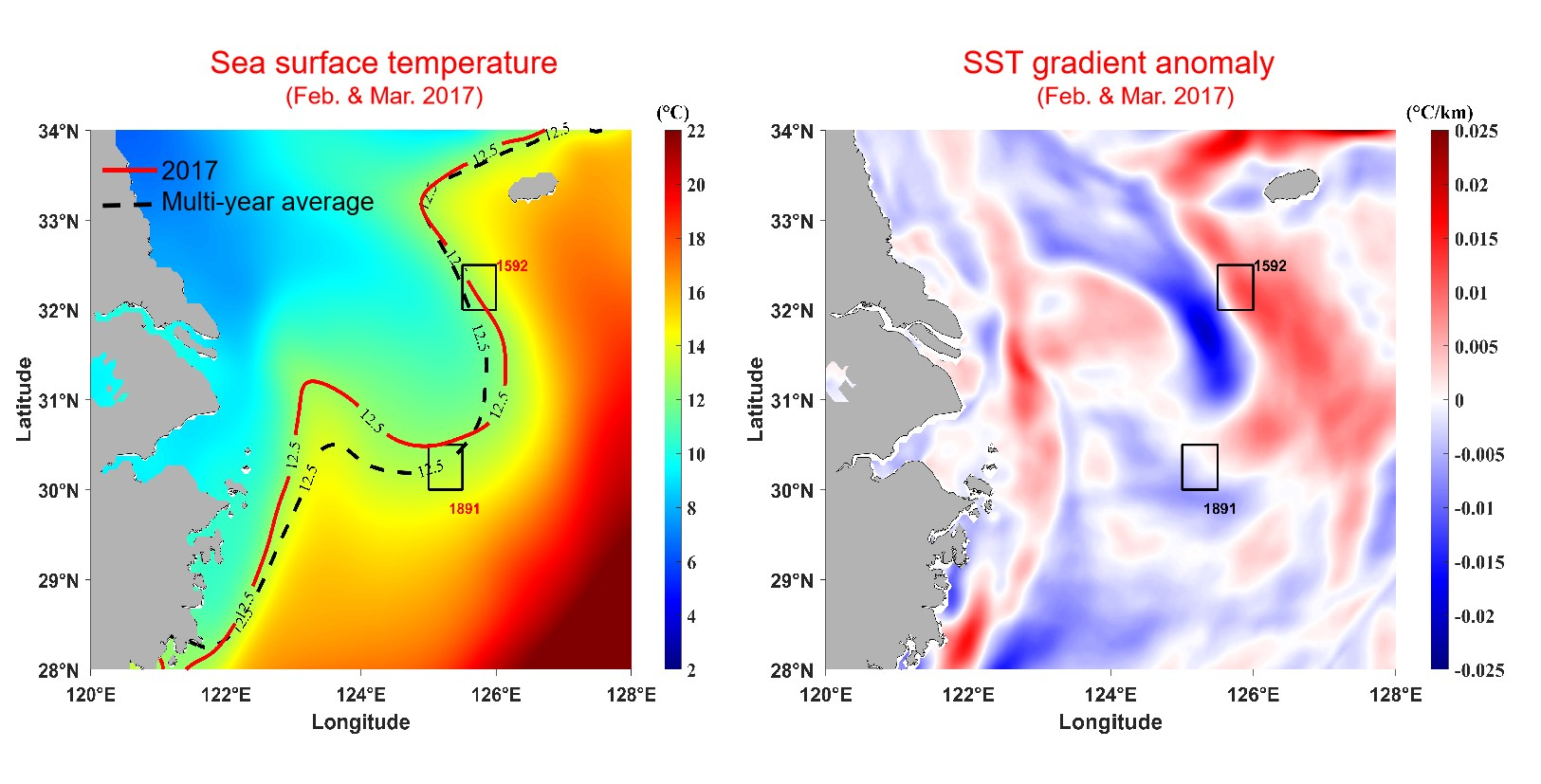
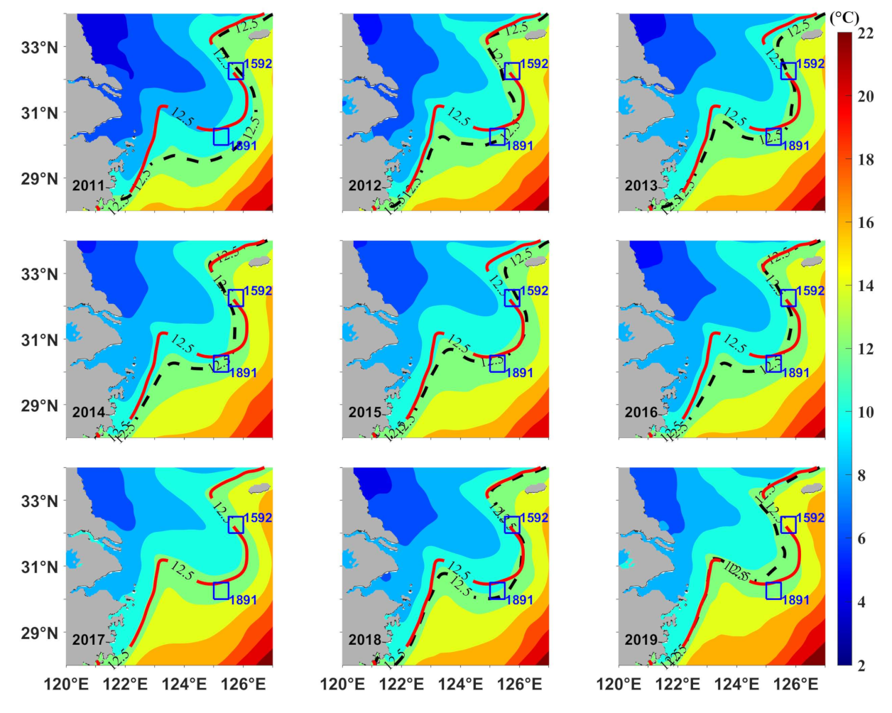
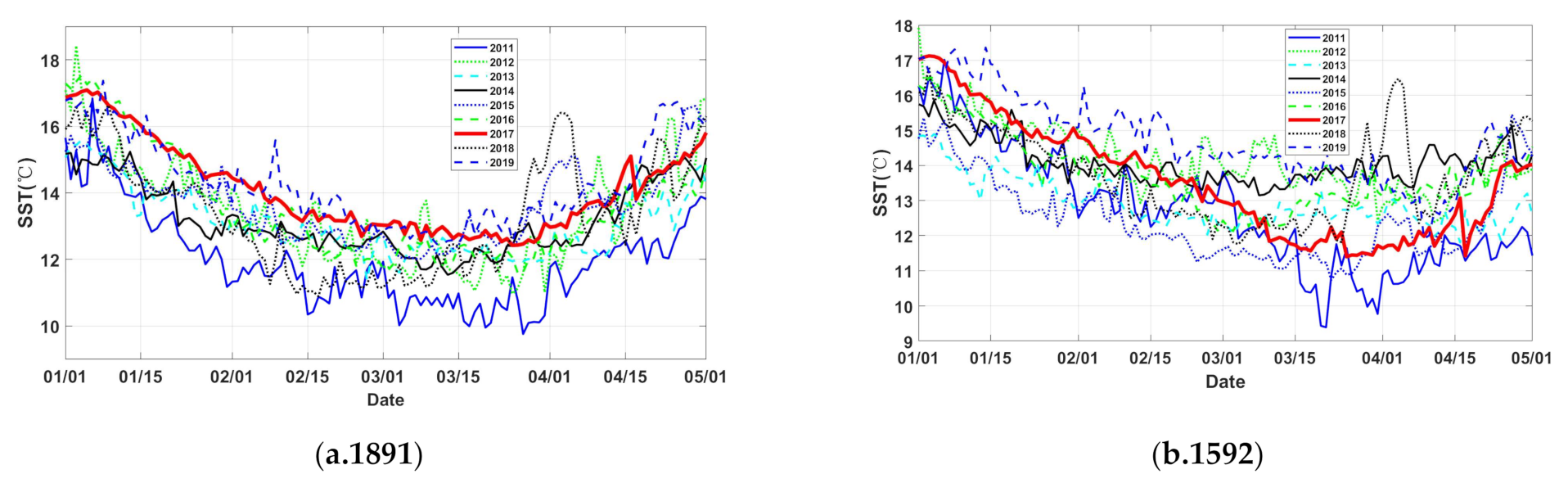
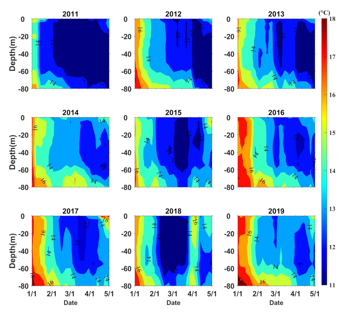
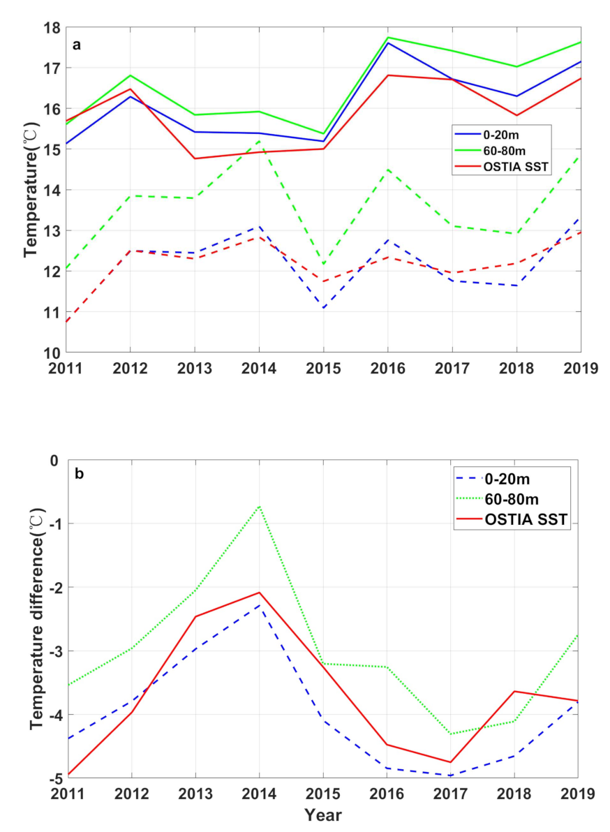
3.1. Temperature
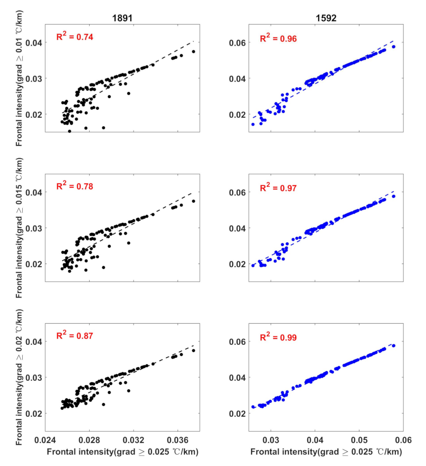
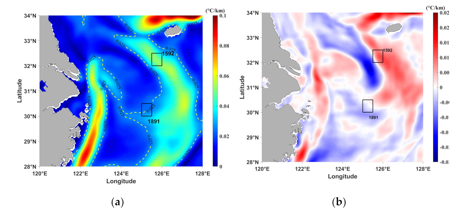
3.2. Thermal Fronts
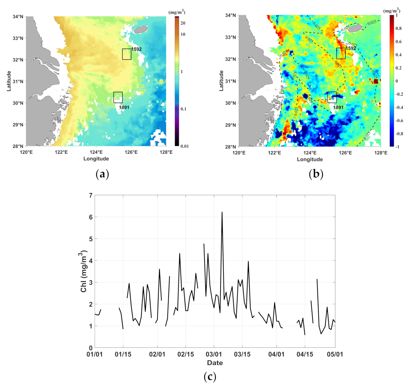
3.3. Chl a
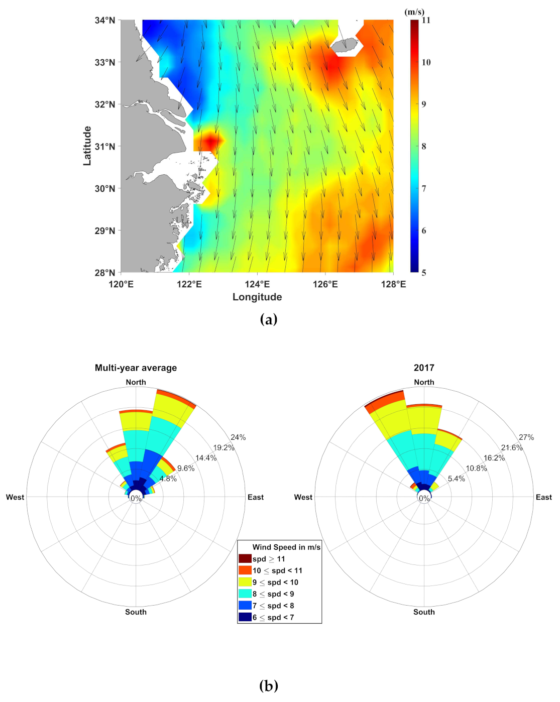
3.4. Wind
4. Discussion
5. Conclusions
Author Contributions
Funding
Data Availability Statement
Acknowledgments
Conflicts of Interest
References
- Lie, H.-J.; Cho, C.-H. Recent advances in understanding the circulation and hydrography of the East China Sea. Fish. Oceanogr. 2002, 11, 318–328. [Google Scholar] [CrossRef]
- Drinkwater, K.F.; Tremblay, M.J.; Comeau, M. The influence of wind and temperature on the catch rate of the American lobster (Homarus americanus) during spring fisheries off eastern Canada. Fish. Oceanogr. 2006, 15, 150–165. [Google Scholar] [CrossRef]
- Winters, D.B. Offshore Wind Energy Impacts on Fisheries: Investigating Uncharted Waters in Research and Monitoring. Fisheries 2018, 43, 343–344. [Google Scholar] [CrossRef]
- Mills, K.E.; Pershing, A.J.; Brown, C.J.; Chen, Y.; Chiang, F.-S.; Holland, D.S.; Lehuta, S.; Nye, J.A.; Sun, J.C.; Thomas, A.C.; et al. Fisheries Management in a Changing Climate: Lessons From the 2012 Ocean Heat Wave in the Northwest Atlantic. Oceanography 2013, 26, 191–195. [Google Scholar] [CrossRef]
- Sambou, O.S.; Kang, B.; Xu, H.X.; Zhou, Y.D.; Panhwar, S.K. Fish assemblage in the Hairtail Protected Area, East China Sea in relation to environmental variables. Cah. Biol. Mar. 2020, 61, 279–289. [Google Scholar] [CrossRef]
- Huang, M.R.; Ding, L.Y.; Wang, J.; Ding, C.Z.; Tao, J. The impacts of climate change on fish growth: A summary of conducted studies and current knowledge. Ecol. Indic. 2021, 121, 106976. [Google Scholar] [CrossRef]
- Xu, Z.L.; Chen, J.J. Analysis on migratory routine of Larimichthy polyactis. J. Fish. Sci. China 2009, 16, 931–940. [Google Scholar]
- Eveson, J.P.; Hobday, A.J.; Hartog, J.R.; Spillman, C.M.; Rough, K.M. Seasonal forecasting of tuna habitat in the Great Australian Bight. Fish. Res. 2015, 170, 39–49. [Google Scholar] [CrossRef]
- Methven, D.A.; Piatt, J.F. Seasonal abundance and vertical distribution of capelin (Mallotus villosus) in relation to water temperature at a coastal site off eastern Newfoundland. ICES J. Mar. Sci. 1991, 48, 187–193. [Google Scholar] [CrossRef]
- Chang, Y.; Lee, M.-A.; Lee, K.-T.; Shao, K.-T. Adaptation of fisheries and mariculture management to extreme oceanic environmental changes and climate variability in Taiwan. Mar. Policy 2013, 38, 476–482. [Google Scholar] [CrossRef]
- Hu, X.M.; Xiong, X.J.; Qiao, F.L.; Guo, B.H.; Lin, X.P. Surface current field and seasonal variability in the Kuroshio and adjacent regions derived from satellite-tracked drifter data. Acta Oceanol. Sin. 2008, 27, 11–29. [Google Scholar]
- Zuo, J.; Song, J.; Yuan, H.; Li, X.; Li, N.; Duan, L. Impact of Kuroshio on the dissolved oxygen in the East China Sea region. J. Oceanol. Limnol. 2018, 37, 513–524. [Google Scholar] [CrossRef]
- Yang, X.M.; Yao, T.D. The progress on the Asian monsoon study. Chin. J. Nat. 1999, 6, 3–5. [Google Scholar]
- Ichikawa, H.; Beardsley, R.C. The Current System in the Yellow and East China Seas. J. Oceanogr. 2002, 58, 77–92. [Google Scholar] [CrossRef]
- Park, S.; Chu, P.C. Thermal and haline fronts in the Yellow/East China Seas: Surface and subsurface seasonality comparison. J. Oceanogr. 2006, 62, 617–638. [Google Scholar] [CrossRef]
- Chen, C.T.A. Chemical and physical fronts in the Bohai, Yellow and East China seas. J. Mar. Syst. 2009, 78, 394–410. [Google Scholar] [CrossRef]
- He, S.; Huang, D.; Zeng, D. Double SST fronts observed from MODIS data in the East China Sea off the Zhejiang–Fujian coast, China. J. Mar. Syst. 2016, 154, 93–102. [Google Scholar] [CrossRef]
- Chang, Y.; Lee, M.A.; Shimada, T.; Sakaida, F.; Kawamura, H.; Chan, J.W.; Lu, H.J. Wintertime high-resolution features of sea surface temperature and chlorophyll-a fields associated with oceanic fronts in the southern East China Sea. Int. J. Remote Sens. 2008, 29, 6249–6261. [Google Scholar] [CrossRef]
- Huang, D.; Zhang, T.; Zhou, F. Sea-surface temperature fronts in the Yellow and East China Seas from TRMM microwave imager data. Deep. Sea Res. Part II Top. Stud. Oceanogr. 2010, 57, 1017–1024. [Google Scholar] [CrossRef]
- Zhao, C.Y. Marine Fishery Resource of China; Zhejiang Science and Technology Press: Hangzhou, China, 1990. (In Chinese) [Google Scholar]
- Zheng, J.Y.; Chen, X.Z.; Cheng, J.H. Fisheries Resource and Environment of Continental Shelf in East China Sea; Shanghai Science and Technology Press: Shanghai, China, 2003. (In Chinese) [Google Scholar]
- Cheng, J.; Cheung, W.W.; Pitcher, T.J. Mass-balance ecosystem model of the East China Sea. Prog. Nat. Sci. 2009, 19, 1271–1280. [Google Scholar] [CrossRef]
- Kang, J.-S. Analysis on the development trends of capture fisheries in North-East Asia and the policy and management implications for regional co-operation. Ocean Coast. Manag. 2006, 49, 42–67. [Google Scholar] [CrossRef]
- Zheng, B.; Chen, X.J.; Li, G. Relationship between the resource and fishing ground of mackerel and environmental factors based on GAM and GLM models in the East China Sea and Yellow Sea. J. Fish. China 2008, 32, 379–386. [Google Scholar]
- Li, G.; Chen, X.; Lei, L.; Guan, W. Distribution of hotspots of chub mackerel based on remote-sensing data in coastal waters of China. Int. J. Remote. Sens. 2014, 35, 4399–4421. [Google Scholar] [CrossRef]
- Lin, H.-Y.; Chiu, M.-Y.; Shih, Y.-M.; Chen, I.-S.; Lee, M.-A.; Shao, K.-T. Species composition and assemblages of ichthyoplankton during summer in the East China Sea. Cont. Shelf Res. 2016, 126, 64–78. [Google Scholar] [CrossRef]
- Liu, K.-K.; Chao, S.-Y.; Lee, H.-J.; Gong, G.-C.; Teng, Y.-C. Seasonal variation of primary productivity in the East China Sea: A numerical study based on coupled physical-biogeochemical model. Deep. Sea Res. Part II Top. Stud. Oceanogr. 2010, 57, 1762–1782. [Google Scholar] [CrossRef]
- Zhang, C.-I.; Seo, Y.-I.; Kang, H.-J.; Lim, J.-H. Exploitable carrying capacity and potential biomass yield of sectors in the East China Sea, Yellow Sea, and East Sea/Sea of Japan large marine ecosystems. Deep. Sea Res. Part II Top. Stud. Oceanogr. 2019, 163, 16–28. [Google Scholar] [CrossRef]
- Teh, L.S.L.; Cashion, T.; Cheung, W.W.L.; Sumaila, U.R. Taking stock: A Large Marine Ecosystem perspective of socio-economic and ecological trends in East China Sea fisheries. Rev. Fish Biol. Fish. 2020, 30, 269–292. [Google Scholar] [CrossRef]
- Jiang, Y.Z.; Cheng, J.H.; Li, S.F. Temporal changes in the fish community resulting from a summer fishing moratorium in the northern East China Sea. Mar. Ecol. Prog. Ser. 2009, 387, 265–273. [Google Scholar] [CrossRef]
- Chen, W.Z.; Zheng, Y.Z.; Chen, Y.Q.; Mathews, C.P. An assessment of fishery yields from the East China Sea Ecosystem. Mar. Fish. Rev. 1997, 59, 1–7. [Google Scholar]
- FAO. The State of World Fisheries and Aquaculture; FAO: Rome, Italy, 1997; p. 125. [Google Scholar]
- Edwards, M.; Richardson, A.J. Impact of climate change on marine pelagic phenology and trophic mismatch. Nat. Cell Biol. 2004, 430, 881–884. [Google Scholar] [CrossRef]
- Perry, A.L.; Low, P.J.; Ellis, J.R.; Reynolds, J.D. Climate Change and Distribution Shifts in Marine Fishes. Science 2005, 308, 1912–1915. [Google Scholar] [CrossRef]
- Tebaldi, C.; Hayhoe, K.; Arblaster, J.M.; Meehl, G.A. Going to the Extremes. Clim. Chang. 2006, 79, 185–211. [Google Scholar] [CrossRef]
- Sukgeun, J.; Hyung, K.C. Fishing vs. Climate Change: An example of filefish (Thamnaconus modestus) in the northern east China sea. J. Mar. Sci. Technol. 2013, 21, 15–22. [Google Scholar] [CrossRef]
- Wall, C.C.; Muller-Karger, F.E.; Roffer, M.A.; Hu, C.; Yao, W.; Luther, M.E. Satellite remote sensing of surface oceanic fronts in coastal waters off west–central Florida. Remote. Sens. Environ. 2008, 112, 2963–2976. [Google Scholar] [CrossRef]
- Straka, W.; Seaman, C.J.; Baugh, K.; Cole, K.; Stevens, E.; Miller, S.D. Utilization of the Suomi National Polar-Orbiting Partnership (NPP) Visible Infrared Imaging Radiometer Suite (VIIRS) Day/Night Band for Arctic Ship Tracking and Fisheries Management. Remote. Sens. 2015, 7, 971–989. [Google Scholar] [CrossRef]
- Cozzolino, E.; Lasta, C.A. Use of VIIRS DNB satellite images to detect jigger ships involved in the Illex argentinus fishery. Remote. Sens. Appl. Soc. Environ. 2016, 4, 167–178. [Google Scholar] [CrossRef]
- Waluda, C.M.; Griffiths, H.J.; Rodhouse, P.G. Remotely sensed spatial dynamics of the Illex argentinus fishery, Southwest At-lantic. Fish. Res. 2008, 91, 196–202. [Google Scholar] [CrossRef]
- Cooke, S.; Lennox, R.; Bower, S.; Horodysky, A.; Treml, M.; Stoddard, E.; Donaldson, L.; Danylchuk, A. Fishing in the dark: The science and management of recreational fisheries at night. Bull. Mar. Sci. 2017, 93, 519–538. [Google Scholar] [CrossRef]
- Hammerschlag, N.; Meyer, C.; Grace, M.; Kessel, S.; Sutton, T.; Harvey, E.; Paris-Limouzy, C.; Kerstetter, D.; Cooke, S. Shining a light on fish at night: An overview of fish and fisheries in the dark of night, and in deep and polar seas. Bull. Mar. Sci. 2017, 93, 253–284. [Google Scholar] [CrossRef]
- Elvidge, C.D.; Baugh, K.; Zhizhin, M.; Hsu, F.C.; Ghosh, T. VIIRS night-time lights. Int. J. Remote. Sens. 2017, 38, 5860–5879. [Google Scholar] [CrossRef]
- Mulet, S.; Rio, M.-H.; Mignot, A.; Guinehut, S.; Morrow, R. A new estimate of the global 3D geostrophic ocean circulation based on satellite data and in-situ measurements. Deep. Sea Res. Part II Top. Stud. Oceanogr. 2012, 77–80, 70–81. [Google Scholar] [CrossRef]
- Guinehut, S.; Dhomps, A.-L.; Larnicol, G.; Le Traon, P.-Y. High resolution 3-D temperature and salinity fields derived from in situ and satellite observations. Ocean Sci. 2012, 8, 845–857. [Google Scholar] [CrossRef]
- Kim, S.H.; Choi, B.K.; Kim, E. Study on the Behavior of the Water Temperature Inversion Layer in the Northern East China Sea. J. Mar. Sci. Eng. 2020, 8, 157. [Google Scholar] [CrossRef]
- Solomon, O.O.; Ahmed, O.O. Fishing with light: Ecological consequences for coastal habitats. Int. J. Fish. Aquat. Stud. 2016, 4, 474–483. [Google Scholar]
- Du, J.-L.; Yang, S.-L.; Feng, H. Recent human impacts on the morphological evolution of the Yangtze River delta foreland: A review and new perspectives. Estuarine, Coast. Shelf Sci. 2016, 181, 160–169. [Google Scholar] [CrossRef]
- Lin, L.; Liu, Z.; Jiang, Y.; Huang, W.; Gao, T. Current status of small yellow croaker resources in the southern Yellow Sea and the East China Sea. Chin. J. Oceanol. Limnol. 2011, 29, 547–555. [Google Scholar] [CrossRef]
- Chen, J.-J.; Xu, Z.-L.; Chen, X.-Z. The spatial distribution pattern of fishing ground for small yellow croaker in China Seas. J. Fish. China 2010, 34, 236–244. [Google Scholar] [CrossRef]
- Liu, X. The Research of Small Yellow Croaker (Larimichthys polyactis) Geographic Race and Gonad; Science Press: Beijing, China, 1962; pp. 35–70. [Google Scholar]
- Li, X.D. A preliminary study on the division of water-system and fishing grounds during winter in the south of Huanghai Sea and the East China Sea. Mar. Forecast. Serv. 1985, 2, 67–72. [Google Scholar]
- Liu, Z.L.; Yuan, X.W.; Yang, L.L.; Yan, L.P.; Tian, Y.J.; Chen, J.H. Effect of climate change on the fisheries community pattern in the overwintering ground of open waters of northern East China Sea. Chin. J. Appl. Ecol. 2015, 26, 901–911. [Google Scholar] [CrossRef]
- Xu, Z.L.; Wang, R.; Chen, Y.Q. Study on ecology of meso-small pelagic copepods in the Southern Yellow Sea and the East Chi-na Sea I. Quantitative distribution. J. Fish. China 2003, 27, 1–8. [Google Scholar] [CrossRef]
- Yatsu, A.; Watanabe, T.; Ishida, M.; Sugisaki, H.; Jacobson, L.D. Environmental effects on recruitment and productivity of Japanese sardine Sardinops melanostictus and chub mackerel Scomber japonicus with recommendations for management. Fish. Oceanogr. 2005, 14, 263–278. [Google Scholar] [CrossRef]
- Yukami, R.; Ohshimo, S.; Yoda, M.; Hiyama, Y. Estimation of the spawning grounds of chub mackerel Scomber japonicus and spotted mackerel Scomber australasicus in the East China Sea based on catch statistics and biometric data. Fish. Sci. 2009, 75, 167–174. [Google Scholar] [CrossRef]
- Guo, A.; Yu, W.; Chen, X.J.; Qian, W.G.; Li, R.C. Relationship between spatio-temporal distribution of chub mackerel Scomber japonicus and net primary production in the coastal waters of China. Acta Oceanol. Sin. 2018, 40, 42–52. [Google Scholar] [CrossRef]
- Liu, F.; Chu, T.; Wang, M.; Zhan, W.; Xie, Q.; Lou, B. Transcriptome analyses provide the first insight into the molecular basis of cold tolerance in Larimichthys polyactis. J. Comp. Physiol. B 2019, 190, 27–34. [Google Scholar] [CrossRef]
- O’Gorman, E.J.; Ólafsson, Ó.P.; Demars, B.O.L.; Friberg, N.; Guðbergsson, G.; Hannesdóttir, E.R.; Jackson, M.C.; Johansson, L.S.; McLaughlin, Ó.B.; Ólafsson, J.S.; et al. Temperature effects on fish production across a natural thermal gradient. Glob. Chang. Biol. 2016, 22, 3206–3220. [Google Scholar] [CrossRef]
- Friedland, K.D.; Langan, J.A.; Large, S.I.; Selden, R.L.; Link, J.S.; Watson, R.A.; Collie, J.S. Changes in higher trophic level productivity, diversity and niche space in a rapidly warming continental shelf ecosystem. Sci. Total. Environ. 2020, 704, 135270. [Google Scholar] [CrossRef]
- Moser, H.G.; Smith, P.E. Larval fish assemblages of the California Current region and their horizontal and vertical distribu-tions across a front. Bull. Mar. Sci. 1993, 53, 645–691. [Google Scholar]
- Sournia, A. Pelagic biogeography and fronts. Prog. Oceanogr. 1994, 34, 109–120. [Google Scholar] [CrossRef]
- Okazaki, Y.; Nakata, H. Effect of the mesoscale hydrographic features on larval fish distribution across the shelf break of East China Sea. Cont. Shelf Res. 2007, 27, 1616–1628. [Google Scholar] [CrossRef]
- Bost, C.; Cotté, C.; Bailleul, F.; Cherel, Y.; Charrassin, J.; Guinet, C.; Ainley, D.; Weimerskirch, H. The importance of oceanographic fronts to marine birds and mammals of the southern oceans. J. Mar. Syst. 2009, 78, 363–376. [Google Scholar] [CrossRef]
- Kindong, R.; Wu, J.; Gao, C.; Dai, L.; Tian, S.; Dai, X.; Chen, J. Seasonal changes in fish diversity, density, biomass, and assemblage alongside environmental variables in the Yangtze River Estuary. Environ. Sci. Pollut. Res. 2020, 27, 25461–25474. [Google Scholar] [CrossRef]
- Yeh, S.W.; Kim, C.H. Recent warming in the yellow/East China Sea during winter and the associated atmospheric circulation. Cont. Shelf Res. 2010, 30, 1428–1434. [Google Scholar] [CrossRef]
- Cai, R.; Tan, H.; Kontoyiannis, H. Robust surface warming in offshore China seas and its relationship to the east Asian mon-soon wind field and ocean forcing on interdecadal time scales. J. Clim. 2017, 30, 8987–9005. [Google Scholar] [CrossRef]
- Cai, R.; Tan, H.; Qi, Q. Impacts of and adaptation to inter-decadal marine climate change in coastal China seas. Int. J. Clim. 2015, 36, 3770–3780. [Google Scholar] [CrossRef]
- Qi, L.; Hu, C.; Wang, M.; Shang, S.; Wilson, C. Floating Algae Blooms in the East China Sea. Geophys. Res. Lett. 2017, 44, 11–501. [Google Scholar] [CrossRef]
- Su, J.L. A review of circulation dynamics of the coastal oceans near China. Acta Oceanol. Sin. 2001, 4, 1–16. [Google Scholar]
- Guan, B.; Fang, G. Winter counter-wind currents off the southeastern China coast: A review. J. Oceanogr. 2006, 62, 1–24. [Google Scholar] [CrossRef]
- Weisberg, R.H.; Zheng, L.; Liu, Y. Basic tenets for coastal ocean ecosystems monitoring. In Coastal Ocean Observing Systems; Academic Press: Cambridge, MA, USA, 2015; pp. 40–57. [Google Scholar] [CrossRef]
- IPCC. Climate Change 2007: The Physical Science Basis, Contribution of Working Group I to the Fourth Assessment Report of the Intergovernmental Panel on Climate Change; Solomon, S., Qin, D., Manning, M., Chen, Z., Marquis, M., Averyt, K.B., Tignor, M., Miller, H.L., Eds.; Cambridge University Press: New York, NY, USA, 2007. [Google Scholar]
- Strüssmann, C.A.; Conover, D.O.; Somoza, G.M.; Miranda, L.A. Implications of climate change for the reproductive capacity and survival of New World silversides (family Atherinopsidae). J. Fish Biol. 2010, 77, 1818–1834. [Google Scholar] [CrossRef] [PubMed]
- Brander, K.M. Cod Gadus morhua and climate change: Processes, productivity and prediction. J. Fish Biol. 2010, 77, 1899–1911. [Google Scholar] [CrossRef] [PubMed]
- Belkin, I.M. Rapid warming of Large Marine Ecosystems. Prog. Oceanogr. 2009, 81, 207–213. [Google Scholar] [CrossRef]
- Liu, Q.; Zhang, Q. Analysis on long-term change of sea surface temperature in the China Seas. J. Ocean Univ. China 2013, 12, 295–300. [Google Scholar] [CrossRef]
- Bao, B.; Ren, G. Climatological characteristics and long-term change of SST over the marginal seas of China. Cont. Shelf Res. 2014, 77, 96–106. [Google Scholar] [CrossRef]
- Nye, J.; Link, J.; Hare, J.; Overholtz, W. Changing spatial distribution of fish stocks in relation to climate and population size on the Northeast United States continental shelf. Mar. Ecol. Prog. Ser. 2009, 393, 111–129. [Google Scholar] [CrossRef]
- Liu, Y.G.; Kerkering, H.; Weisberg, R. Coastal Ocean Observing Systems; Academic Press: London, UK, 2015. [Google Scholar]


Publisher’s Note: MDPI stays neutral with regard to jurisdictional claims in published maps and institutional affiliations. |
© 2021 by the authors. Licensee MDPI, Basel, Switzerland. This article is an open access article distributed under the terms and conditions of the Creative Commons Attribution (CC BY) license (https://creativecommons.org/licenses/by/4.0/).
Share and Cite
Ding, W.; Zhang, C.; Hu, J.; Shang, S. Unusual Fish Assemblages Associated with Environmental Changes in the East China Sea in February and March 2017. Remote Sens. 2021, 13, 1768. https://doi.org/10.3390/rs13091768
Ding W, Zhang C, Hu J, Shang S. Unusual Fish Assemblages Associated with Environmental Changes in the East China Sea in February and March 2017. Remote Sensing. 2021; 13(9):1768. https://doi.org/10.3390/rs13091768
Chicago/Turabian StyleDing, Wenxiang, Caiyun Zhang, Jianyu Hu, and Shaoping Shang. 2021. "Unusual Fish Assemblages Associated with Environmental Changes in the East China Sea in February and March 2017" Remote Sensing 13, no. 9: 1768. https://doi.org/10.3390/rs13091768
APA StyleDing, W., Zhang, C., Hu, J., & Shang, S. (2021). Unusual Fish Assemblages Associated with Environmental Changes in the East China Sea in February and March 2017. Remote Sensing, 13(9), 1768. https://doi.org/10.3390/rs13091768