1. Introduction
Land use, land cover and their changes are among the most relevant environmental variables [
1,
2] with an influence on topics of crucial importance such as global change and land management at all spatial scales [
1].
Remote sensing imagery classification is generally used to monitor land use and land cover on the Earth’s surface. Currently, the availability of a wide range of spaceborne optical and radar systems has boosted the use of multi-spectral and multi-sensor imagery with high temporal and spatial resolution from different satellites and has generalized studies aiming to improve land cover classification accuracy. The Sentinel program from the European Spatial Agency (ESA) is one of the most recent missions focusing on many different aspects of Earth observation, including land monitoring [
3].
Sentinel-2 (S2) consists of two twin-polar orbiting satellites (Sentinel-2A and 2B) active since 2018 [
4,
5]. They contain a Multi-Spectral Instrument (MSI) that samples 13 spectral bands including visible, near-infrared and shortwave infrared. Having two satellites allows for a high temporal resolution (five days at the Equator and 2–3 days under cloud-free conditions in midlatitudes). The spatial resolution is 10 m in the visible and near-infrared bands. Several studies [
6,
7,
8,
9] have tested these images with good results due to their better temporal and spatial resolution and a complete interoperability with previous satellite programs such as Landsat [
4].
Semiarid Mediterranean regions, due to their socio-economic and physical characteristics, have a high spatial irregularity in their landscape, including a variety of spatial patterns, high fragmentation and a wide range of vegetation coverage [
10,
11]. These characteristics pose a challenge for remote sensing classification. The distinction between crops and natural vegetation, rainfed and irrigated crops or some anthropogenic surfaces is a complex issue to solve, worsened by the spectral properties of lithology, soils and different vegetation species. This issue has been usually addressed using spectral indices, which emphasize surface biophysical characteristics [
12,
13], or texture features extracted from an image [
10]. Additionally, Reference [
11] used a multi-temporal approach with one image per season to include a wider range of spectral properties per class. Their results reported an improvement in the separability between vegetation classes.
A good pre-processing is essential for multi-temporal classification and retrieval of surface biophysical parameters from optical images [
14]. Atmospheric correction (AC) is the most important step in this process, as most satellites currently include good quality radiometric and geometric corrections. The aim of applying AC is to remove atmospheric effects from images, leaving only the surface reflectance values [
15,
16].
However, atmospheric conditions and effects are quite different depending on several factors for each different study area. It is then a difficult task to obtain a good AC, especially for multi-spectral data acquired at high spatial resolution [
17,
18,
19]. It is also important to take into account other issues such as the adjacency effect, which results in a reduction of the contrast between bright and dark pixels because of the light scattered from neighbouring pixels. Such issues might reduce apparent resolution and classification accuracy [
20].
For these reasons, researchers from many institutions across Europe have developed a wide range of algorithms for atmospheric correction [
21]. In recent years, several studies have been conducted to compare the reflectivity of Level-2A (L2A) images, processed with different AC algorithms, with ground truth reflectivity [
14,
19,
22]. In addition, NASA and ESA, in the framework of the Committee on Earth Observation Satellites (CEOS), have initiated an Atmospheric Correction Inter-Comparison Exercise (ACIX) [
23] to analyse several current AC algorithms and to compare the quality of their surface reflectance products. During this study, arid sites were found quite challenging because of the absence of dark dense vegetation pixels and a general underestimation of aerosols; hence, performance at those sites was the main problem for all AC algorithms examined. Among the AC algorithms for S2 evaluated in ACIX were MACCS and Sen2Cor, both resulting among the four in better performances at all sites [
23]. A recent study analysed the performance of MAJA, Sen2Cor and others compared with in situ measurements of an area in the central sector of the Ebro Basin in Zaragoza, Spain [
22]. Although the methods’ performances ranked differently for different land covers, the results showed minor differences overall. However, a study performed by [
24] pointed out difficulties determining the most accurate model for correction due to several factors that might jeopardize a proper comparison. Among others, one of the most important problems is that field measurements are likely to be taken on a unique material, while measurements from remote sensors are taken on different materials due to the spatial resolution. In regions with high landscape fragmentation, as the Mediterranean areas, this problem implies that the reflectance values of a satellite image might mix values coming from more than one land use or cover.
The studies carried out so far were devoted to finding the best AC method to reproduce ground truth spectral signatures. No studies, as far as we know, have tried to analyse how AC methods affect the classification accuracy or class separability. It is generally assumed that land cover and land use classification of a single-date image, or even when images from different seasons are used to obtain a single land cover map, might not need an atmospheric correction, depending on the purpose of the study and, of course, the quality of the data [
25]. However, we believe that AC might increase class separability and therefore classification accuracy.
The aim of this study was to compare classification accuracy after using different AC algorithms in a semiarid Mediterranean area and to analyse how these algorithms might increase class separability in the feature space. According to previous studies, the selected algorithms: Sen2Cor, ACOLITE, MAJA and DOS have shown good performances in similar environments or have been developed specifically to deal with tasks such as the adjacency effect or to improve the recognition of water surfaces. We applied them to S2 Level-1C (L1C) imagery for land use and cover classification in the southeast area of the Hydrographic Demarcation of the Segura River (DHS). In addition, other typical strategies to increase classification accuracy (using images of several dates and using normalized indices) have been tested in order to compare their effects on classification accuracy. In order to keep the results simple, we did not test the results of AC methods in each season individually, but only in two cases: three seasons (excluding winter) and four seasons.
2. Methodology
2.1. Study Area
The study area is a 100 × 100 km
2 portion of the T30SXG S2 granule that includes the southern coast of the Hydrographic Demarcation of the Segura River (DHS), in Southeast Spain (
Figure 1). The annual mean rainfall is 382 mm, although the high spatial and temporal variability of rainfall results in the usual alternation of extreme droughts and floods. Temperatures are warm throughout the year, with a mean ranging from 10 °C to 17–18 °C and a thermal amplitude between 12 and 17 °C. There is a wide range of different orographic and climatic features, lithology and soil classes and vegetation covers, both natural and anthropic. The population is about 1 million inhabitants, concentrated in the Guadalentin Valley and the coastal areas, included in this granule.
The main uses in the study area are urban and agricultural. The area belongs to the Murcia Region and represents more than a quarter of its surface and half of its total population, including two of the most populated and largest urban areas. Along the coast, both large, urbanised surfaces (tourist resorts) are intermingled with some protected coastal mountain ranges. That implies a seasonal increase in population that is hardly quantifiable.
Besides, it includes two of the main agricultural areas in the Murcia Region: the Cartagena countryside and the Guadalentin Valley, where fields of irrigated crops alternate with dense tree crops of citrus in lower slope areas. Such covers represent more than 51,800 ha. Rainfed crops and low dense tree fields are found in the foothills of the central mountain ranges of the region, and those are located in the north and northwest sectors of the granule and represent a total of 9575 ha. Crops under plastic and greenhouses are almost 17,500 ha in the study area [
26].
2.2. Atmospheric Correction Algorithms and Processors
Sentinel data are available as top of atmosphere (TOA) reflectance values. L2A products with bottom of atmosphere (BOA) values, estimated with the Sen2Cor algorithm, have also been distributed since 2017. Other algorithms widely used for S2 and included in this study are dark object subtraction (DOS), the most used image-based method for atmospheric correction, MAJA and ACOLITE. The two latter are physically-based methods.
2.2.1. Sen2Cor
Sen2Cor [
27] is an algorithm developed by ESA specifically for Sentinel 2 satellites, and the code is freely available as a SNAP (Sentinel Application Platform) plugin. Users can also obtain L2A products corrected with the Sen2Cor algorithm by downloading them directly from Copernicus Open Access Hub.
The algorithm performs a cloud detection and a scene classification, followed by a retrieval of aerosols and water vapour from L1C images. BOA reflectivity values are then obtained using those values. The scene classification module does not produce a land cover map strictly speaking, but a map with 11 classes including cloud, bright and water pixels, obtained using the dark dense vegetation (DDV) method [
28]. Sen2Cor depends on two ancillary variables: the look up tables of radiative transfer (LUT) and the digital elevation model (DEM).
Sen2Cor is the most accessible of all AC algorithms tested here. Images already corrected with this method can be downloaded from the Copernicus web site (
https://scihub.copernicus.eu/dhus/#/home (accessed on 21 July 2020)). It can also be applied to L1C images using SNAP, where Sen2Cor can be implemented as a plugin; giving the user the possibility of changing the default parameters. The images used in this study were corrected before we downloaded them.
2.2.2. MACCS-ATCOR Joint Algorithm
MAJA is a MACCS-ATCOR joint algorithm [
29], whose complete description can be found in [
30,
31], as well as in the Algorithmic Theoretical Basis Document (ATBD) [
32]. Multi-Temporal Atmospheric Correction and Cloud Screening software (MACCS) is an algorithm developed by the Centre d’Etudes Spatiales de la Biosphère (CESBIO) and the Centre National d’Etudes Spatiales (CNES) as a multi-spectral and multi-temporal AC method. ATCOR is another AC software developed by the Deutsche Zentrum für Luft und Raumfahrt (DLR). The method uses as the input a DEM, which helps in determining absorption or Rayleigh scattering, detecting shadows, clouds and cirrus, masking water and determining aerosol optical thickness (AOT). It can additionally use ozone data if available, but default values are used if not. It is a very complicated algorithm, highly demanding of computer resources and programming knowledge. Fortunately, the French THEIA Data and Services Center has integrated MAJA in its process of the generation of L2A products, so it can be used to process images with the code freely distributed or by downloading already processed images from the THEIA web page (
https://www.theia-land.fr/en/product/sentinel-2-surface-reflectance/ (accessed on 30 April 2021)).
2.2.3. Dark Object Subtraction
DOS is a widely used family of simple image-based AC methods. It is based on the assumption that if dark objects, such as water or dense vegetation, are in complete shadow and have zero reflectance, the value registered by the sensor must be only due to atmospheric scattering [
33]. Hence, the minimum digital number from a scene is considered as a dark object and its value considered as the atmospheric effect. There are different DOS techniques for correction, depending on the minimum percentage value assumed as radiance in dark objects; for DOS1, it is 1%. The problem is that the initial assumption itself might be wrong, as in inland images in semiarid areas, where dense vegetation is rarely found. As it is a basic and well-known method for correction, it is usually implemented in almost every Geographical Information System (GIS). Therefore, to carry out this correction, the DOS1 processor in the Semi-Automatic Classification Plugin for QGIS was used [
34].
2.2.4. ACOLITE
ACOLITE [
35,
36,
37] was created to process Landsat and S2 data for water applications and coastal areas. It is based on the dark spectrum fitting (DSF) algorithm, which has two main assumptions: the homogeneity of atmospheric conditions over a certain area and the existence of pixels with a near-zero value in at least one band. The lowest value obtained from every other band is used to build a dark spectrum as a base of an aerosol model calculated by linear interpolation. After a process of various steps, fully described in [
36], the surface reflectance is retrieved. The estimated air-water interface sky reflectance is set to 0 in land pixels and analytically estimated in water pixels.
2.3. Data Sets
One image from every season in the hydrologic year 2018–2019 was selected (
Table 1). Images were downloaded from Copernicus Open Access Hub repository in Level 1C (L1C) with TOA values and Level 2A (L2A) already corrected to BOA values with Sen2Cor. ACOLITE correction for S2 L1C images was run with the interface and code freely distributed by the Remote Sensing and Ecosystem Modelling (REMSEM) team. Finally, the DOS correction was applied to L1C images using the Semi-Automatic Classification Plugin (SCP) for QGIS [
34].
From the 13 bands collected by MSI, only those with a 10 and 20 m spatial resolution (
Table 2) were used. The latter were resampled to a 10 m resolution using the nearest neighbour method.
Using indices to recognise biophysical patterns on the Earth’s surface is a common and effective practice supported by a wide range of studies [
38,
39,
40,
41,
42,
43]. Indices highlight basic interactions between spectral variables. Hence, some indices were included in the data set:
The normalized difference vegetation index (
NDVI) [
44] is a much used index for measuring and monitoring vegetation cover and biomass production with satellite imagery. It is calculated with Equation (
1).
where
is a narrow near-infrared band (NIR) for vegetation detection and
the red band (R) from S2A MSI.
Tasselled cap brightness (
TCB) [
45] tries to emphasize spectral information from satellite imagery. Spectral bands from the visible and infrared (both near and shortwave) spectra are used to obtain a matrix that highlights brightness, greenness, yellowness, nonesuch [
45] and wetness [
46] coefficients. In this case, we used the brightness equation, also known as the soil brightness index (SBI), which detects variations in soil reflectance. The equation for S2 is:
where
,
and
are the blue (B), green (G) and red (R) bands;
is the NIR band; and
and
are the SWIR from S2A MSI.
The soil adjusted vegetation index (
SAVI) [
47]: Due to the NDVI’s sensitivity to the proportion of soil and vegetation, this index adds to the NDVI a soil factor. In semiarid areas, this is a way to fit the index to background average reflectance. The equation is:
where
is the NIR band,
the R band and
L is a factor for soil brightness with a value of 0.5 to fit with the majority of covers.
The normalized difference built-up index (
NDBI) [
48] is used to distinguish built surfaces, which receive positive values, from bare soils. It is calculated with Equation (
4).
where
is the SWIR band and
the NIR band.
The modified normalized difference water index (
MNDWI) [
49] was proposed to detect superficial water. However, due to the relation between SWIR and wetness in soils, it can be also used to detect water in surfaces of vegetation or soil. The index is calculated with Equation (
5).
where
is the G band and
the SWIR band.
2.4. Training Areas and Classification Scheme
Training areas were selected using the most recent aerial orthophotography from the Spanish Plan Nacional de Ortofotografía Aerea (PNOA) (Aerial Orthophotography National Plan) (
https://pnoa.ign.es (accessed on 30 April 2021)). Polygons for every class were distributed homogeneously, balanced all over the DHS to include its spectral heterogeneity, avoiding statistical dependence. After that, the representativity for all areas was enhanced following the methodology proposed in [
50], resulting in a total of 209 polygons distributed into a ratio of 70/30 for training and validation. The classification scheme adopted (
Table 3) was decided by grouping diverse covers to obtain a feasible set that was representative at a regional scale.
2.5. Classification Accuracy
Random forest (RF) [
51] is a non-parametric method based on an ensemble of decision trees, usually between 500 and 2000, with two procedures to reduce correlation among trees: (1) each tree is trained with a bootstrapped subsample of the training data; (2) the feature used to split each node of the trees is selected from a randomly generated subset of features. Once all trees are calibrated, each one contributes with a vote to classify every new pixel. Finally, the pixel is assigned to the most voted class.
The algorithm also produces an internal form of cross-validation and a ranking of the importance of the different variables to increase classification accuracy. It is calculated by measuring how the accuracy decreases when a feature is randomly reshuffled while the rest remains unchanged [
52].
RF is a robust method for supervised classification [
11], although when the number of variables or predictors is quite high, it is advisable to increase the default number of decision trees, to avoid high variability in the variables’ importance.
The randomForest library [
52] of the R [
53] program was used. It allows setting parameters and applying the algorithm over big data sets. We also used the caret library [
54] to obtain confusion matrices and other accuracy statistics. The parameters of the model are
ntree, the number of trees in the forest (500 by default), and
mtry, the number of predictors from which we selected the one that increased the homogeneity in each node (square root of the number of predictors by default) [
52]. We used the default value for
mtry and 2000 for
ntree.
Our main objectives were to test if the AC methods introduce a significant increase in classification accuracy, to identify the methods whose increase is significantly higher than others and to compare those increases with those produced by the use of 4, instead of 3, images, as well as by the introduction of spectral indices. The null hypotheses were that no difference resulted in the introduction of such methods.
In order to evaluate the accuracy of the classifications, we used overall accuracy, which is the proportion of corrected classified cases, and the kappa index [
55], defined as:
where
n is the sample size,
the correctly classified cases in each class
i and
the expected agreement in each class
i. Kappa index ranges from 0 (the classification is as good as random) to 1 (the classification is perfect). Values lower than 0 are possible, but very rare. Reference [
56] stated that kappa values can be classified as: 0.00–0.20, insignificant; 0.21–0.40, low; 0.41–0.60, moderate; 0.61–0.80, good; and 0.81–1.00, very good.
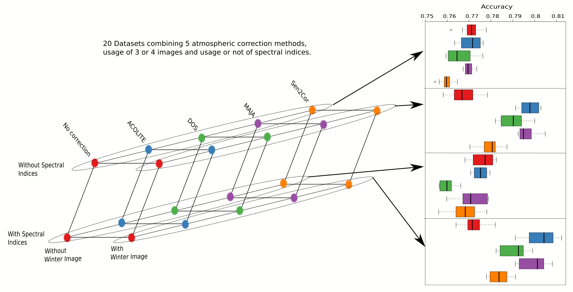
Twenty different data sets were generated resulting in 5 different AC algorithms (including no correction) and 4 different feature sets (including or not the winter image and including or not normalized indices). These data sets included 10 reflectivity features and 5 indices. Therefore, the number of features ranged from 30 (no winter image and no indices) to 60 (winter image and indices).
In order to estimate the statistical significance of recorded accuracy differences, ten replications of the validation results were produced by bootstrapping. An ANOVA analysis to check for accuracy equality was conducted with these replications after testing for residual normality and homoscedasticity (using the Kolmogorov–Smirnov and Levene tests, respectively). Besides establishing which factors are significantly different, the 20 combinations of factors were grouped into data sets with no significantly different accuracy. Such a grouping was carried out from the results of multiple pair comparison based on a Tukey–Kramer contrast.
2.6. Separability Analysis
Class separability in the feature space is an important issue in remote sensing imagery classification. The Jeffries–Matusita (JM) distance [
57] is the usual approach to measure class separability. It can be expressed as:
where
is the Bhattacharyya distance between classes
i and
j. Usually, a multivariate normal distribution is assumed [
58], and this distance is estimated as:
where
is the vector of reflectivity means for class
i and
the covariancematrix of class
i. The JM distance reaches asymptotically 2 when the two classes are completely separable and is zero when they are the same. However, the JM distance assumes multivariate normality in each of the classes [
59], and such assumption is difficult to assess, especially in multi-image classification, and difficult to fulfil.
Reference [
50] proposed a different approach using isolation forests (IFs) [
60] to evaluate how representative of the study area a training data set is and also to estimate the separability between classes using the proportion named the common isolation value (CIV) as a parameter to measure the separability. If an IF model is trained with a sample of data, it will produce a metric of how novel any new case in the context of that sample is. If trained with pixels of one class, it can be used to measure how different any other pixel is compared to that class. A low CIV means that it is very different, and a high CIV means that it is very similar. If we compare the CIV distributions of two classes A and B estimated with an IF model calibrated with one of them (B for instance), the overlapping of both distribution curves measures how easily both classes may be confused (
Figure 2). We estimated the CIV parameter as the ratio between the intersection of both curves and the union of the curves.
CIV has proven to be more informative than the JM distance, not only stating which classes are similar and more likely confused within the extent of each other, but also predicting omission and commission errors [
50]. The lower the CIV of the IF, the better the separability between classes.
We also used a new metric based on a nearest neighbour distance approach that we called the between-class nearest neighbour distances (BCNND) index. The distance of each point in Class A to its nearest neighbour in Class B is compared to the nearest neighbour distances of all points in Class B. The probability of obtaining such a distance, or larger, if both points are of Class B is computed as a measure of how separate that Class A point is from the cloud formed by the Class B points. Finally, the proportion of Class A points with a probability equal to or lower than 0.99 is a measure of how separate Class A is from Class B. The threshold is not really that important because increasing or decreasing it will increase or decrease all the proportions, and the final ranks would be similar.
The algorithm can be summarised as:
Compute the nearest neighbour distances for each class.
Compute the distance of all points in Class A to their nearest neighbour in Class B
Compute the probability of such distances being equal or higher than its value assuming that they belonged to Class B.
Compute the percentage of cases with a probability larger than 0.99 ()
Repeat Steps 2 to 4 for all pair combinations
As the measure is not reciprocal, that is , the final BCNNDindex is then computed as the weighted average of and .
Separability analysis with the Jeffries–Matusita distance was carried out by season instead of using the whole data set. The reason was that the Jeffries–Matusita distance, when calculated with the whole data set, reached the highest possible value showing a very low variance. The Jeffries–Matusita distance assumes multivariate normality in the per-class reflectivity distributions [
59]. We think that the failure to comply with this condition was the reason for these anomalous results. The CIV-based separability analysis was carried out seasonally to compare with the JM distance. Twenty-five bootstrapping resamples were extracted to obtain an empirical probability distribution of the JM distance and the CIV.
Being quite more computationally demanding, no replication was carried out for the BCNND index, but it was also calculated for the whole data set instead of seasonally.
3. Results
3.1. Corrected Data Sets
The new reflectance data sets resulting from the application of different AC methods to the L1C data set were quite similar and to L1C, except in the visible bands, especially the blue band (B02), which showed major corrections. Although it is important to remember that we were operating at a regional scale, most of the classes were quite heterogeneous, and the spectral reflectances had a high variance.
Figure 3 shows some signatures able to help clarify confusions between crops, bare soils, impermeable and greenhouses. All signatures were quite similar regardless the atmospheric correction method employed. Low-density tree crops and rainfed grass crops (both rainfed) had very similar patterns. However, some differences could be found: an increase in the mean reflectivity in Band 11 (SWIR) with respect to Band B08A (NIR) for rainfed grass crops in autumn and a wider inter-quantile range in the spring image for low-density tree crops. Dense tree crops and irrigated grass crops (both irrigated) also showed a strong similarity, the difference being the higher variability in irrigated grass crops. These facts made these two classes extremely prone to being confused. Interestingly, when the data were corrected with a physically-based method, the winter image appeared to be the only one that showed a small distinction between classes by the type of irrigation (irrigated or rainfed), whether having slight differences of the values in the red edge and NIR band in the rainfed classes or the NIR and VIS bands in the case of irrigated classes.
Physical-based methods, Sen2Cor, MAJA and ACOLITE, tended to uniformise the values in the red edge (B05, B06, B07) and NIR (B08 and B08A) with respect to the values without correction, while the values corrected with DOS were closer to those that were not corrected, even showing similar patterns. The visible band’s reflectivities were reduced after correction, except for B02 for artificial or bare soil surfaces, while NIR and SWIR tended to increase. The reflectivity values were higher in spring and summer, except for the impermeable and bare soil classes, which remained almost the same in every single season. However, major atmospheric corrections were found in the winter image, in which the corrected values differed from the uncorrected one in the majority of bands and classes.
Greenhouses’ spectral patterns were similar to those of irrigated grass crops, especially in the autumn and winter images, whereas they were more related to those of impermeable and bare soil in spring and summer. The last two had almost exactly the same values in the mean and quantiles, except for slight differences in the quantile of 95. The class signature with a lower range was dense tree crops. Bare soils and impermeable were almost exactly equal to each other.
Slight differences in Band B08A in the autumn image and in Bands B08A and B11 in the spring image were found for both rainfed classes. There was a lower inter-quantile range for dense tree crops in the autumn, winter and summer images with respect to the irrigated grass crops class. In addition, irrigated grass crops had means and quantiles almost equal to greenhouses in autumn and winter images. Bare soil and impermeable also showed similar signature patterns, impermeable having a higher inter-quantile range.
By the atmospheric correction method, there were slight differences between the data corrected for each class. In fact, were barely found a class where there was any overlap with other classes. The ranges were quite high, which indicated high variance in most of the classes. The highest values and ranges were in impermeable, greenhouses, bare soil and low-density tree crops in data corrected with Sen2Cor, mainly in spring and summer scenes. ACOLITE correction seemed to produce lower reflectivity inter-quantile ranges than the others, which could be related to the larger class separability and higher classification accuracy.
3.2. Classification Accuracy
Table 4 shows the average values of global accuracy and the kappa index for the different AC methods and data sets and the 95% uncertainty intervals calculated from a representative confusion matrix. The classification accuracy seemed to increase, in general, with bands corrected by ACOLITE, closely followed by MAJA. Uncertainty was low and very similar for every other classification, but slightly lower for ACOLITE and MAJA with the complete data sets (four seasons and indices). Its decreasing with the addition of variables indicated the utility of the variables added. The results of the analysis of variance of accuracy with bootstrapped resampling showed significant differences (
in all cases).
Figure 4 and
Table 5 show the different effects that were found to be significant.
Figure 4 shows accuracy distributions obtained with 10 resamplings of the 20 combinations of AC, the use of indices and the number of seasons. The lower-case letters above the boxes represent the non-significantly different groups to which each combination belonged, obtained with ANOVA after the multiple pair comparison based on a Tukey–Kramer contrast. The groups
i and
j were those with the highest accuracy and were comprised by ACOLITE and MAJA using winter images, with or without spectral indices. The highest accuracy values were obtained with ACOLITE and the indices, but the differences with the other three were not significant.
Table 5 shows the magnitude of the different effects and interactions that were found significant. The greatest effect was observed when ACOLITE was used compared to when the images were not corrected (0.029), followed by the use of MAJA (0.024) and the inclusion of the winter season (0.019). The effect of using indices, on the contrary, seemed not to be relevant.
It is interesting that when no winter image was used, using AC did not seem to increase the classification accuracy; it actually reduced it, especially in the cases of DOS and Sen2Cor. However, when the winter image was included in the data set, the accuracy increased significantly, especially when ACOLITE or MAJA were used. Adding normalized indices did not seem to significantly increase the accuracy in these cases. We think that, being a semiarid area, AC did not make a difference except for winter images as the presence of the sea introduced a large amount of coastal mist.
Figure 5 shows the per-class accuracy distributions obtained with 10 resamplings of the 20 combinations; lower-case letters above the boxes are used with the same meaning as in
Figure 4.
Table 6 summarises
Figure 5 showing, in each class, which combinations appeared in the group with the most accurate combinations. Water surfaces were classified with high accuracy independently of the combination used. Accuracy for natural surfaces seemed to increase when no indices were used; however, although the differences were statistically significant, their magnitude was quite low. Cultivated classes had the largest differences between combinations. In these classes, the highest accuracy was reached with MAJA and Sen2Cor in low-density tree crops, ACOLITE and MAJA in high-density tree crops, MAJA in rainfed grass crops and ACOLITE and Sen2Cor in irrigated grass crops and greenhouses. Impermeable areas showed a different result, as DOS was the AC algorithm that reached a higher accuracy with a substantial difference in relation to the other methods. Bare soil areas reached higher accuracy without the winter image and without indices using whichever method (even no correction), except DOS.
The difference between the maximum accuracy and the minimum accuracy (
Table 6) showed that, independently of the statistical significance, some classes, such as low-density tree crops, dense tree crops and irrigated grass crops, experienced larger increases in accuracy (larger than 0.15), while in others, such as forest, scrub or greenhouses, the accuracy increase was very modest (lower than 0.05). Interestingly, the classes with a larger accuracy increase were the agricultural classes, which were more difficult to separate and at the same time usually more relevant.
3.3. Separability Analysis
The results by season using the JM distance or the CIV did not show any significant difference in mean separability, but the variances were quite different and the distributions skewed towards high separability values (around 1.4 in the Jeffries–Matusita distance and zero in the CIV). An example showing the results for the separability of low-density tree crops and dense tree crops appears in
Figure 6. Therefore, the best option would be to chose the lowest variance method. The Levene test, using the median instead of the average as the centrality statistic, was used to test differences in variance. The Levene test was less sensitive to non-normality than other equal variance tests [
61], and using the median increased its robustness.
As we used the JM distance and the CIV to measure class separability in each season, the results were too complex to introduce all of them in a figure. Instead, we summarize the results in
Figure 7 and
Figure 8, which show how many times each combination of the AC algorithms, combined with the usage or not of spectral indices, appeared in the group of the lowest JM distance or the CIV variances estimated with the Levene test. The results of both class separability measurements were less correlated than expected. According to the results of the Jeffries–Matusita index, ACOLITE was the best AC method to increase class separability. It was the best option in all seasons; in some cases, using indices, but in others, without the inclusion of indices. However, the results of the CIV showed that no correction provided a better separability than ACOLITE, although ACOLITE appeared as the second best option and MAJA the third. These disparate results using the CIV or the JM distance can be related to two issues. Firstly, the JM distance results may be affected by the non-normality of the distributions. On the other hand, both statistics might be measuring different things, and more research is needed for this issue.
The probability distributions of the distances to the nearest neighbour computed for each class are presented in
Figure 9. The highest distances appeared in urban areas and greenhouses and the lowest in water and cultivated areas. These distances gave an idea of the scatter of the pixel clouds in the feature space. All empirical distributions could be modelled using a log-normal model.
Figure 10 shows the BCNND index results for the least separable combinations of classes. The BCNND index ranges from zero (very large separability) to one (very low separability) and represents the proportion of pixels that are prone to be confused. The value of the BCNND index for the class pairs not included was near zero in all cases.
Using DOS decreased the class separability in most of the class pairs, and it seemed that it was better to use no correction instead of using DOS. There were several class combinations that did not change separability regardless of the AC method or the predictors included: scrub vs. urban and scrub vs. greenhouses. Urban and bare soil were the most easily confused classes, and no method was able to solve the problem. ACOLITE including winter images (but without indices) and MAJA without the winter image and without indices reduced the index to around 0.64. The inclusion of the winter image increased separability for dense tree crop vs. irrigated grass crops, rainfed grass crops vs. irrigated grass crops and irrigated vs. urban. The inclusion of indices seemed to improve the results in scrub vs. bare soil, dense tree crop vs. greenhouses, irrigated vs. bare soil, bare soil vs. greenhouses and rainfed vs. bare soil. Finally, the inclusion of the winter image and indices had a positive effect for irrigated grass crops vs. greenhouses and bare soil vs. greenhouses. It is noteworthy that, however, both the inclusion of a fourth winter image and the inclusion of indices decreased the separability in forest vs. scrub.
Figure 11 shows the average of the results shown in
Figure 10. DOS was the method with the worst results, and ACOLITE, when including winter images and indices, obtained the best results. Any method, except DOS using the winter image, with or without indices, was the next best option.
The main disadvantage of this method comparing with the JM distance or the CIV was that it was quite more time consuming. That was the reason why no resampling was used to calculate its statistical distribution.
4. Discussion
Most of the previous studies comparing AC methods were based on ground truth reflectivity. However, in this study, we calculated the classification accuracy and class separability using different AC methods in order to evaluate their performance. Therefore, the results were not directly comparable in a quantitative way. However, our results were qualitatively in line with those of recent studies on the inter-comparison of AC methods using reflectivity field samples.
Spectral signatures corrected with DOS were very similar to the uncorrected one, as in [
14,
19]. Image-based methods rely ultimately on the subtraction of dark dense vegetation (DDV) pixels from TOA data, so the shape of spectral signatures may no differ from data without correction. The scarcity of dense vegetation in semiarid Mediterranean territories jeopardizes the effectiveness of this method and explains the poor performance in accuracy and separability for almost every class. Although we verified a good performance for impermeable surfaces, as was found in [
14], our results for bare soil were much worse than theirs. This may be due to the existence of sparse vegetation, the diversity of mineral composition or the colour of the bedrock over bare soil surfaces.
On the other hand, data corrected with physically-based methods were in agreement with each other, but were quite dissimilar to non-corrected data, as these methods also tended to homogenise values in the red edge and NIR bands. ACOLITE and MAJA produced the best classification accuracy and separability for most of the classes, especially for crops. ACIX [
23] tested several AC methods, including ACOLITE, MAACS (the former version of MAJA) and Sen2Cor, and compared their performance for Sentinel-2 data correction at different sites around the world. Unfortunately, as the sites were selected among locations included in the Aerosol Robotic Network (AERONET) to have the availability of reliable atmospheric information for validation, arid sites were included, but no semiarid. Some of the coastal sites analysed in their study share, to a certain extent, some climatic characteristics with our study area, and all three of them were tested in them. Unfortunately, while Sen2Cor performed accurately with respect to true reflectance surfaces, especially in the visible bands, it was not possible to achieve proper results for MACCS and ACOLITE due to the absence of sufficient data. The study developed by [
22], over five land covers, also included in our classification scheme, using, among others, MAJA and Sen2Cor, stated MAJA as a better option for correction over Sen2Cor, especially for vegetation covers. Our results showing an improvement in accuracy per class using images from the four seasons corrected with MAJA was coherent with the conclusions of [
23].
In our study, ACOLITE outperformed MAJA in overall accuracy and separability in most of the classes when the data set included the winter image and indices. However, MAJA was the second best option as it still outperformed ACOLITE in separability in some of the most important classes of crops. The lack of previous inter-comparison studies including ACOLITE and MAJA with sufficient data to establish a proper comparison is noteworthy.
The best classification result in overall accuracy was from ACOLITE, although considering results by class, MAJA outperformed it in some of the classes. Moreover, as the study area is a coastal area with most of its surface covered by crop fields and urban areas, these results seemed to be consistent with the fact that the main purpose of ACOLITE is to perform atmospheric correction in coastal areas. If the study area had extended to other areas of the DHS, the results could have been different. For this reason, MAJA should not be discarded as an atmospheric correction method. Its use for correcting optical images of Sentinel2 jointly with SAR data (Sentinel 1) has already been implemented in applications for agriculture, as Sen2Agri [
62,
63,
64,
65]. More predictors, algorithms and methods should be tested to achieve better rates of separability.
5. Conclusions
The main purpose of this study was to test the best AC method to improve classification accuracy and class separability in a semiarid Mediterranean coastal area. The most confounding classes included crops, artificial surfaces, and bare soil. This issue has been previously reported in several multitemporal studies and addressed in different ways, such as adding indices and ancillary or textural variables as predictors [
10,
11,
12,
13]. However, we tried a different approach, comparing the results of using different AC methods, as well as including different variables in each data set.
The largest effect detected on accuracy was the use of ACOLITE as the atmospheric correction method, followed by the use of MAJA, the use of three seasons and, finally, the use of indices. Therefore, atmospheric correction seems to be a key step in order to improve classification accuracy. The analysis of spectral signatures showed that DOS, the most widely AC method, produced very few changes on reflectivity, whereas physically-based methods produced similar results to each other and different from the non-corrected signatures.
When integrating all these effects, the most accurate classification was obtained with ACOLITE-corrected bands, four seasons and indices. However, the results obtained with MAJA, four seasons and indices were not significantly different. There was a clear improvement in accuracy when the winter image was added, but not when the spectral indices were added.
Per-class accuracy values showed a more complex picture. In most of the classes, ACOLITE with indices and the winter image appeared in the group of the most accurate methods. However, in five classes, there was a different result. The class scrub had the highest accuracy using MAJA and the winter image with or without indices. Low-density tree crops reached the highest accuracy with MAJA or Sen2Cor using the winter image both with and without indices. The classes rainfed grass crops and bare soil reached the highest accuracy using MAJA with indices, but no winter image. Finally, the class impermeable reached the highest accuracy using DOS and both the winter image and indices. Summarising these results, ACOLITE was the best option for five classes and MAJA for four classes. The use of indices and the winter image was the best option in most of the classes.
According to the Jeffries–Matusita distance, ACOLITE without indices provided the best separability results in spring and summer images, whereas also ACOLITE, but with indices, was the best option for autumn and winter images.
The results were different for the CIV. In this case, no correction seemed the best option in summer, autumn and winter, whereas ACOLITE with indices was the best option for the spring image. ACOLITE with indices was also the second best option in the other three seasons. In this case, a strange behaviour appeared. On the one hand, a low correlation between the JM distance and the CIV was observed, but on the other hand, although in the case of the CIV, ACOLITE was still the AC method that improved separability the most, it did not improve the separability of the bands. Another aspect to highlight, complementary to the analysis of spectral signatures that we carried out, was that the JM distance and the CIV indicated that DOS even reduced the separability with respect to the uncorrected bands.
The BCNND results were more similar to those of the Jeffries–Matusita distance and those obtained with accuracy. ACOLITE with indices and the winter image was the combination that reached a higher separability, although in general, any method, except DOS, with winter images reached similar separability values. The results per class were more complex as there were class combinations that were hardly separable (scrub and urban, scrub and greenhouses, urban and bare soil and urban and greenhouses) regardless of the AC method or combination of variables used to classify. Scrub and bare soil and bare soil and greenhouses were also difficult to separate, but the separability improved adding the winter image and indices.
The conclusions of this study should not be directly applied to other areas as environmental differences may produce changes in the ranking of the AC methods. It is even possible that the results in this same study area could be different for different images due to the atmospheric situation of every image. However, we think that the methodology could be useful. More studies in other areas are needed before a claim in relation to which AC method works generally best can be made.


