GOSAT CH₄ Vertical Profiles over the Indian Subcontinent: Effect of a Priori and Averaging Kernels for Climate Applications

Abstract

We examined methane (CH₄) variability over different regions of India and the surrounding oceans derived from thermal infrared (TIR) band observations (TIR CH₄) by the Thermal and Near-infrared Sensor for carbon Observation—Fourier Transform Spectrometer (TANSO-FTS) onboard the Greenhouse gases Observation SATellite (GOSAT) for the period 2009–2014. This study attempts to understand the sensitivity of the vertical profile retrievals at different layers of the troposphere and lower stratosphere, on the basis of the averaging kernel (AK) functions and a priori assumptions, as applied to the simulated concentrations by the MIROC4.0-based Atmospheric Chemistry-Transport Model (MIROC4-ACTM). We stress that this is of particular importance when the satellite-derived products are analyzed using different ACTMs other than those used as retrieved a priori. A comparison of modeled and retrieved CH₄ vertical profiles shows that the GOSAT/TANSO-FTS TIR instrument has sufficient sensitivity to provide critical information about the transport of CH₄ from the top of the boundary layer to the upper troposphere. The mean mismatch between TIR CH₄ and model is within 50 ppb, except for the altitude range above 150 hPa, where the sensitivity of TIR CH₄ observations becomes very low. Convolved model profiles with TIR CH₄ AK reduces the mismatch to less than the retrieval uncertainty. Distinct seasonal variations of CH₄ have been observed near the atmospheric boundary layer (800 hPa), free troposphere (500 hPa), and upper troposphere (300 hPa) over the northern and southern regions of India, corresponding to the southwest monsoon (July–September) and post-monsoon (October–December) seasons. Analysis of the transport and emission contributions to CH₄ suggests that the CH₄ seasonal cycle over the Indian subcontinent is governed by both the heterogeneous distributions of surface emissions and the influence of the global monsoon divergent wind circulations. The major contrast between monsoon, and pre- and post-monsoon profiles of CH₄ over Indian regions are noticed near the boundary layer heights, which is mainly caused by seasonal change in local emission strength with a peak during summer due to increased emissions from the paddy fields and wetlands. A strong difference between seasons in the middle and upper troposphere is caused by convective transport of the emission signals from the surface and redistribution in the monsoon anticyclone of upper troposphere. TIR CH₄ observations provide additional information on CH₄ in the region compared to what is known from in situ data and total-column (XCH₄) measurements. Based on two emission sensitivity simulations compared to TIR CH₄ observations, we suggest that the emissions of CH₄ from the India region were 51.2 ± 4.6 Tg year⁻¹ during the period 2009–2014. Our results suggest that improvements in the a priori profile shape in the upper troposphere and lower stratosphere (UT/LS) region would help better interpretation of CH₄ cycling in the earth’s environment.

1. Introduction

The South Asia region, consisting of India, Pakistan, Bangladesh, Nepal, Bhutan, and Sri Lanka, play an import part in the global methane (CH₄) budget, because the regional total emissions contributed 8% (about 500 Tg) of the CH₄ global total emissions during the 2000s [1]. The recent economic growth of India has led to a significant increase in industrial emissions [2,3,4], especially in the Indo-Gangetic Plain (IGP), encompassing northern regions of the Indian subcontinent. The IGP is one of the most densely populated regions with strong emissions of various tracers due to human activity [5]. However, there are little or no long-term measurements of CH₄ and the other greenhouse gases to evaluate the inventory emissions [6,7,8,9].

The Asian Summer Monsoon Anticyclone (ASMA) is a dominant circulation pattern in the Upper Troposphere and Lower Stratosphere (UT/LS) in the northern hemisphere in summer, which extends from Southeast Asia to the Middle East [10,11]. The Asian monsoons may be classified into a few sub-systems, such as the South Asian Monsoon, which affects the Indian subcontinent and surrounding regions. The monsoon is associated with persistent strong convection over India and the Bay of Bengal, elevated surface heating over the Tibetan Plateau, and orographic uplifting at the southern/south-western slopes of the Himalayas, which contributes to overall ascension of boundary layer air to the upper troposphere (up to ~200 hPa) [12]. The deep convection and associated circulation patterns of the monsoon provides an important pathway for polluted boundary layer air to reach UT/LS [13,14]. The atmospheric compounds can then be advected horizontally to other regions, or further uplifted in to the stratosphere [1,8,15,16]. Due to the influence of deep convection and long-range transport, the chemical tracers such as CH₄, CO, and ozone often show extreme values [17,18]. Global observations from satellite instruments can complement and extend the information available from the in situ observations at sparse surface networks and aircraft campaigns to improve our knowledge of the processes controlling the emission and distribution of CH₄, and to monitor its variability on different scales. The shortwave infrared (SWIR) and thermal infrared (TIR) bands are available for measurements of CH₄ from space. Observations in the SWIR, such as those from the Thermal Additionally, Near-infrared Sensor for carbon Observation-Fourier Transform Spectrometer (TANSO-FTS) onboard the Greenhouse gases Observation SATellite (GOSAT) [19,20,21], provide information on column-averaged CH₄ (XCH₄), in cloud-free conditions during the daytime satellite overpass. On the other hand, TIR CH₄ observations provide much greater geographical and temporal coverage, and more importantly, the measurements of vertical profiles would allow a better understanding of the CH₄ cycle over a region. The sensitivity of TIR CH₄ observations is stronger in the mid to upper troposphere and relatively low near the surface, because its spectral signatures depend on thermal contrast between the atmosphere and surface [22,23].

The heterogeneity in surface emissions variations of XCH₄ governed by complex atmospheric transport mechanisms during the southwest monsoon season in July–September and northeast monsoon season in October–December is observed by GOSAT. The work by Chandra et al. [8] has highlighted the difficulty in interpreting the emissions from the surface by columnar CH₄ measurements from SWIR spectra, without using an atmospheric chemistry-transport model. At the same time, Ricaud et al. [24] investigated the impact of the Asian Monsoon Anticyclone to the distribution of the mid-to-upper CH₄ in the Mediterranean Basin using a wide variety of datasets including GOSAT/TANSO-FTS TIR observations.

Critical data for interpretation of satellite retrievals of trace gas are the a priori information on the shape of the vertical profile and the averaging kernel (AK) functions. Both should be implemented to the simulated profile to resample the simulated profile in a manner that mimics the satellite vertical sensitivity [25]. A priori profiles are derived from a chemical transport model or a representation which has different physical processes, emissions, or spatial resolutions. As a result, comparisons between satellite-retrieved and model-simulated column abundances are greatly influenced by the a priori profile shape [26].

This study analyzes the vertical distributions of CH₄ over the Asian monsoon region. We used CH₄ mixing ratios observed from GOSAT/TANSO-FTS TIR (hereafter referred to as “GOSAT-TIR”) Version 1 (Level 2 V1) and simulated by MIROC4.0-based Atmospheric Chemistry-Transport Model (MIROC4-ACTM) for the period from 23 April 2009, until 24 May 2014. We discuss challenges in using GOSAT-TIR CH₄ (hereafter referred to as “TIR CH₄”) data to determine relative contributions of surface emissions and transport in the formation of CH₄ seasonal cycles over different parts of India and the surrounding oceans. The paper is structured as follows. In Section 2, we briefly describe the spaceborne instrument GOSAT-TIR and vertical profile retrievals of CH₄, the MIROC4-ACTM simulation setup, the study domain, and data processing. The meteorology and climatology of CH₄ inferred from the different datasets over the study domain, variability of CH₄ vertical profiles, and the impact of the Asian Monsoon Anticyclone to the distribution of the tropospheric CH₄ are discussed in Section 3. Major conclusions are given in Section 4.

2. Methods

2.1. Study Domain

This work follows the setup described by Chandra et al. [8] and uses 10 regions (Figure 1a) which are characterized by different CH₄ emissions and meteorological conditions. The Indian landmass was partitioned into eight sub-regions surrounded by two oceanic regions. From southwest to northeast, there are: the Arabian Sea (AS), Southern India (SI), the Bay of Bengal (BB), Western India (WI), Central India (CI), Eastern India (EI), Arid India (AI), Western IGP (WIGP), Eastern IGP (EIGP), and Northeast India (NEI).

2.2. GOSAT-TIR Retrievals

GOSAT was the first satellite dedicated to global observations of greenhouse gases CO₂ and CH₄ from space. Since the launch on 23 January 2009, observations are made on a 666 km sun-synchronous orbit with a 3-day revisit cycle, and 12-day operation cycle, with overpasses twice a day at local noon 13:00 ± 15 min and near-midnight [27]. During daytime, GOSAT/TANSO-FTS can simultaneously observe CH₄ column-averaged dry-air mole fractions and CH₄ profiles in the same field of view (a nadir footprint diameter of 10.5 km) using SWIR and TIR spectral bands, respectively [28,29]. Therefore, daytime observations are screened more thoroughly by TANCO-Cloud and Aerosol Imager (CAI). At night, observations and filtering are carried out only by the TIR algorithms. Therefore, the number of scenes of daytime and night-time observations can differ significantly, especially during the monsoon period. However, the average difference between the retrieved CH₄ is usually within ±20 ppb when data within one day are compared. We leave a more detailed analysis of the daily variation of CH₄ outside the scope of this work.

The retrieval algorithm for the GOSAT-TIR V1 CH₄ adopted a nonlinear maximum a posteriori (MAP) method with linear mapping [22]. A priori covariance matrix for CH₄ in the V1 CH₄ retrieval is set to be a diagonal matrix with vertically fixed diagonal elements with a standard deviation of 4%. The first retrieval version of the TIR CH₄ product (Level 2 V00.01) and its validation analysis showed that the TIR XCH₄ profiles were within 0.5% agreement with the aircraft XCH₄ values over the tropical ocean [30]. Work by Holl et al. [31] compared CH₄ data from the Canadian Space Agency’s Atmospheric Chemistry Experiment FTS (ACE-FTS), ground-based FTS, and the current released version of GOSAT-TIR (Level 2 V1) in the Canadian high Arctic, although TIR CH₄ measurement information content is too low for true profile retrieval because of the low thermal contrast and the low signal-to-noise ratio over the Arctic. Zou et al. [32] performed global comparisons with the Atmospheric Infrared Sounder (AIRS) retrievals for the levels of 300–600 hPa, where both AIRS and GOSAT-TIR V1 CH₄ have peak sensitivities. Mean mismatch in CH₄ (GOSAT–AIRS) were 10.3–31.8 and −16.2 ± 25.7 ppbv for the levels of 300 and 600 hPa, respectively. Comparison of the XCH₄ shows that TIR CH₄ agrees with AIRS to within 1% in the mid-latitude regions of the Southern Hemisphere and in the tropics, and to ~1–2% in the mid to high latitudes [32]. Olsen et al. [33] performed global comparisons of GOSAT-TIR V1 CH₄ vertical profiles to ACE-FTS (version 3.5) and the European Space Agency’s Michelson Interferometer for Passive Atmospheric Sounding (MIPAS), as well as 16 ground stations with the Network for the Detection of Atmospheric Composition Change (NDACC). In the overlapping altitude ranges of the three satellite data products there is a small, but consistent, positive bias of around 20 ppbv, or 1% in TIR CH₄ data. In the upper troposphere, no bias between TIR CH₄ and NDACC was found.

In a more recent comparison, the average bias in CH₄ profile retrieved from GOSAT-TIR spectra with a spectral correction scheme was less than 2% over the full altitude range, when compared with data from the Monitoring Atmospheric Composition and Climate (MACC) scaled to the total column measurements of the Total Carbon Column Observing Network (TCCON) [23].

Global comparisons are also conducted based on HIPPO, CARIBIC, JMA, and CONTRAIL/ASE aircraft observations (Saitoh, N. et al.: Intensive validation analysis of GOSAT/TANSO-FTS thermal infrared CH₄ data (version 1) based on aircraft observations, in preparation). In low latitudes corresponding to the India location, compared datasets include CARIBIC profiles over MAA (Chennai, India), BOG (El Dorado, Colombia), and CCS (Venezuela) airports and CONTRAIL/ASE over GUAM (U.S.A.) airport. The validations show that TIR V1 CH₄ and aircraft CH₄ profiles agreed with each other within 10–15 ppb and there was no evident seasonal dependence in the CH₄ differences.

2.3. TIR CH₄ Profile Properties

The observation by GOSAT-TIR band enables analysis of the vertical structure of atmospheric CH₄. This band has relatively high spectral resolution of ~0.2 cm⁻¹ and provides CH₄ vertical profiles in 22 layers from the surface to 0.1 hPa. The degrees of freedom (DOF) of signal for TIR CH₄ observations (V1 algorithm version) is around 1 over low-latitude parts of India. DOF means the number of purely (mathematically) independent pieces of information. However, the real atmospheric layers correlate with each other, so even if its DOF is close to 1, TIR has the ability to derive new knowledge about CH₄ concentrations. Figure 1 shows a typical TIR CH₄ profile with retrieval errors and a priori profile and its corresponding AK profiles for the southern and northeast regions of India, and over the Bay of Bengal during the monsoon season. The a priori profiles (Figure 1b,d,f) used in the CH₄ retrieval were provided by the National Institute for Environmental Studies (NIES) transport model using 47 sigma levels. The stratospheric part of the NIES model was adjusted to the observed age of air for CO₂ and long-term satellite observations from HALOE for CH₄ [34].

Analysis of the AK profiles of the TIR CH₄ products (Figure 1c,e,g) show that the GOSAT-TIR measurement signal is beyond the retrieval error at pressure levels of 500–150 hPa with the sensitivity maximum at the levels of 200–400 hPa decreasing towards the surface. The spectra sensitivity does not change significantly between the different parts of the study domain but becomes low in the lower troposphere (below 800 hPa), emphasizing the major limitation of TIR CH₄ measurements.

2.4. MIROC4-ACTM Simulations

The measurements were compared to results of simulations by the MIROC4-ACTM simulation [35,36]. The MIROC4-ACTM runs at a horizontal resolution of T42 spectral truncations (~2.8 × ~2.8) with 67 sigma-pressure vertical levels. The MIROC4-ACTM simulated horizontal winds (U and V) and temperature (T) are nudged to the Japan Meteorological Agency reanalysis fields (JRA-55) at all the vertical levels [37]. The model uses an optimal OH field based on a scaled version of the seasonally varying OH field [38,39].

Two simulations were performed using combinations of inverted fluxes at monthly intervals, based on two a priori emission scenarios [40]:

• Flux_Cao: EDGAR + GFED + other + VISIT wetland&rice (Cao scheme [41]);
• Flux_WH: EDGAR + GFED + other + VISIT wetland&rice (WH scheme [42]).

The anthropogenic emissions for an individual sector were taken from EDGAR (the Emission Database for Global Atmospheric Research, version 4.3.2 inventory [4]) on an annual basis for the period 1970–2012, and the global total emissions were extrapolated to 2017 using the 2011–2012 rate of change. GFED (Global Fire Database version 4s [43]) provides interannually varying monthly emissions for biomass burning. The other emissions (including ocean, termites, mud volcano, etc.) were taken from the TransCom-CH₄ inter-comparison experiment [44]. While all other emissions were common, the VISIT (Vegetation Integrated Simulator of Trace gases [45,46]) provided two distinct sets of wetland and rice emissions on a monthly basis using two different schemes developed by [41,42], which are referred to as “${\mathrm{ACTM}}_{\mathrm{Cao}}$” and “${\mathrm{ACTM}}_{\mathrm{WH}}$”, respectively (Figure 2). The main difference between these approaches in most cases can be explained by the combined effect of changes in soil temperature and the position of the water table. In general, the emissions WH scheme are about 5–10% larger than those by the Cao scheme, except for the WIGP, EIGP, and NEI regions of India and Bangladesh where the maximum difference reaches 20–40% (Figure 2). Moreover, there are small number of hotspots in Southeast Asia (e.g., Mekong River Delta region), in the case of Cao scheme compared to WH scheme.

2.5. Data Processing

The MIROC4-ACTM simulations were sampled and collocated in space and time to the TIR CH₄ observation points. The criteria for the collocation were the nearest model grid cell in space, and the nearest hour in time. For vertical profile comparison, the MIROC4-ACTM data were interpolated on the retrieval pressure levels of the TIR CH₄ product, i.e., from 67 model levels to 22 retrieval levels.

2.6. AK Functions and the Retrieval Sensitivity

AK functions are defined to provide a simple characterization of the relationship between the retrieval and the true state. The retrieval sensitivity can be obtained from the sum of the columns of the AK matrix, which is also referred to as “the area of the averaging kernel” [25]. Along with “raw” model simulation results (${\mathrm{ACTM}}_{\mathrm{Cao},\mathrm{WH}}$), we analyzed (${\mathrm{ACTM}}_{\mathrm{Cao},\mathrm{WH}}^{\mathrm{AK}}$) profiles convolved with retrieval a priori and the TIR CH₄ AK matrix using the following vector equation [25,30]:

$$X_{{\mathrm{ACTM}}_{\mathrm{Cao},\mathrm{WH}}^{\mathrm{AK}}}=X_{a priori}+A\left(X_{{\mathrm{ACTM}}_{\mathrm{Cao},\mathrm{WH}}}-X_{a priori}\right),$$

(1)

Here, A is an AK matrix, X_{a priori} represents a vector of an a priori vertical profile, and $X_{{\mathrm{ACTM}}_{\mathrm{Cao},\mathrm{WH}}}$ and $X_{{\mathrm{ACTM}}_{\mathrm{Cao},\mathrm{WH}}^{\mathrm{AK}}}$ are vectors of “raw” and convolved model simulated profiles, respectively.

2.7. The Prophet Analysis and Forecasting Model

TIR CH₄ observations show large temporal and spatial heterogeneity, which complicate the derivation of seasonal cycle variation. The Prophet is a novel time-series analysis and forecasting model [47], which performs the smoothing of time-series data based on a generalized additive model with three main properties: trend, seasonality, and holidays. Compared to traditional exponential smoothing, Prophet can handle temporal patterns with multiple periods and has no requirements regarding the regularity of measurement spacing. The model has a robust performance in the presence of missing data and trend shifts, and typically handles outliers well while working with time-series that have several seasons of historical data with strong seasonal patterns. Prophet managed to use all data points for the study period, thereby increasing accuracy and reducing the sensitivity to random outliers [48].

3. Results

3.1. Prevailing Atmospheric Conditions over the Indian Subcontinent

Key components of the climatology in the Indian Ocean and the surrounding areas are the annual migration of the Intertropical Convergence Zone (ITCZ) and seasonal development of monsoon winds [10,11,49,50]. In boreal spring, the ITCZ migrates northward across the Indian Ocean and reaches its northernmost position at approximately 35°N during summer. A strong pressure gradient between the low-pressure zone over the Tibetan Plateau and a high-pressure zone over the Southern Indian Ocean generates a strong near-surface monsoonal airflow from July to September (Figure 3c1–c3). In autumn, the ITCZ retreats southward and reaches its southernmost position in January. The reversed pressure gradient during the winter months generates the moderate and dry northeast monsoon (Figure 3d1–d3). Devasthale and Fueglistaler [51] showed that a significant fraction of high opaque clouds reaches and penetrates the tropical tropopause layer during active ASMA conditions (Figure 3c). The overall frequency of convective clouds (reaching at least 200 hPa) is higher in July and August. Most of the deep convection occurs over the Bay of Bengal and central northeast India [52], while very deep convection over the Tibetan plateau is comparatively weak, and may play only a secondary role in troposphere-to-stratosphere transport.

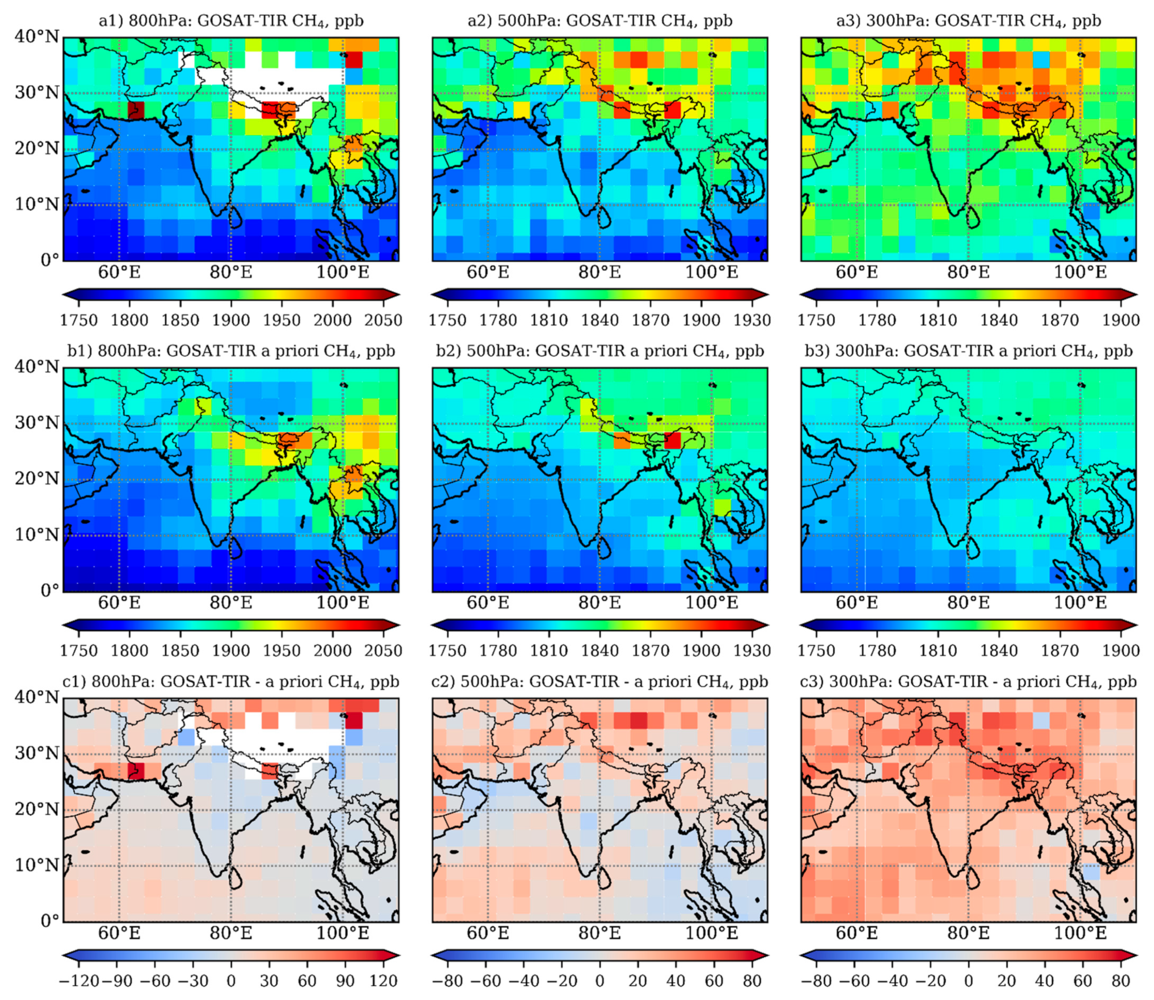
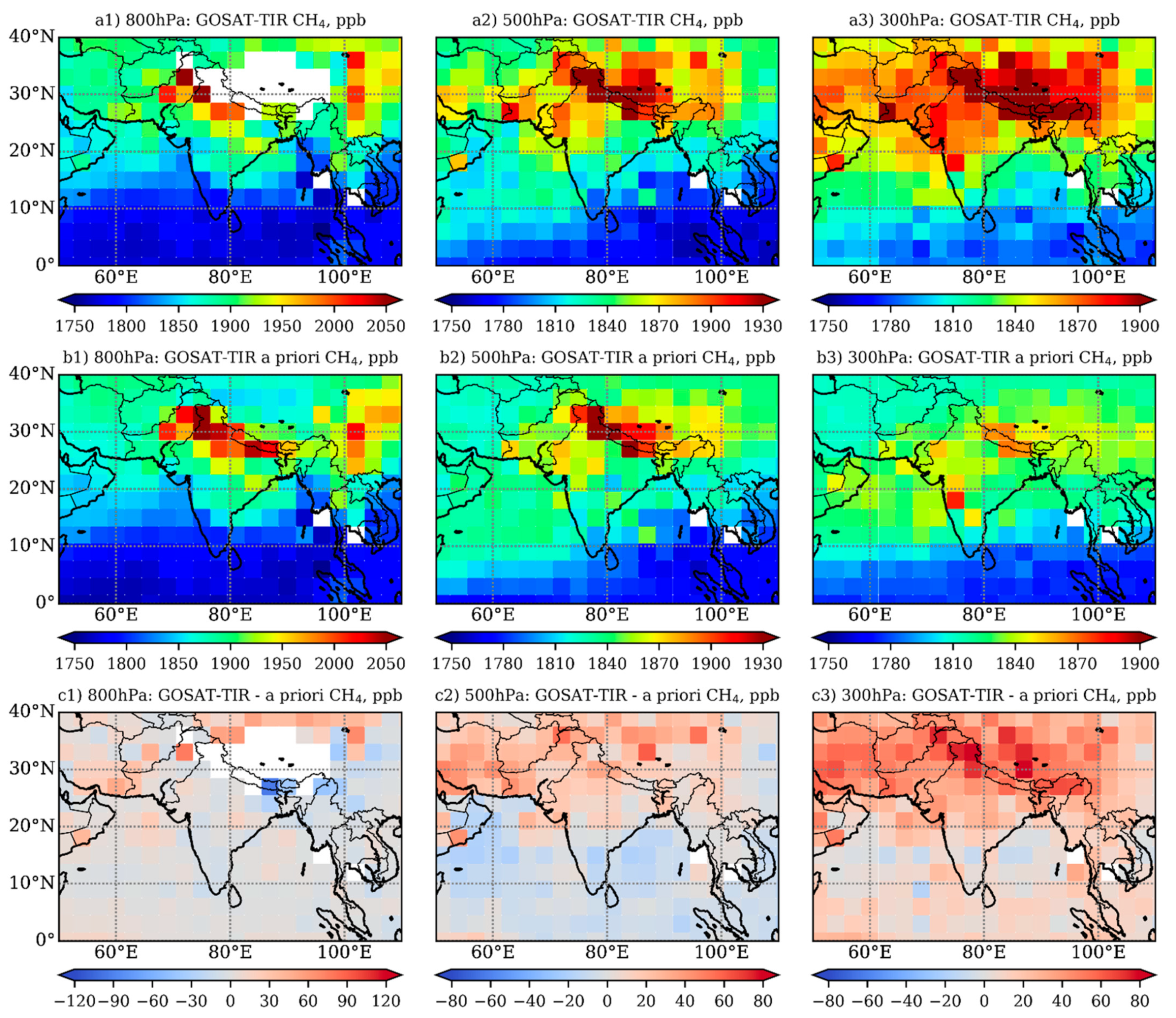
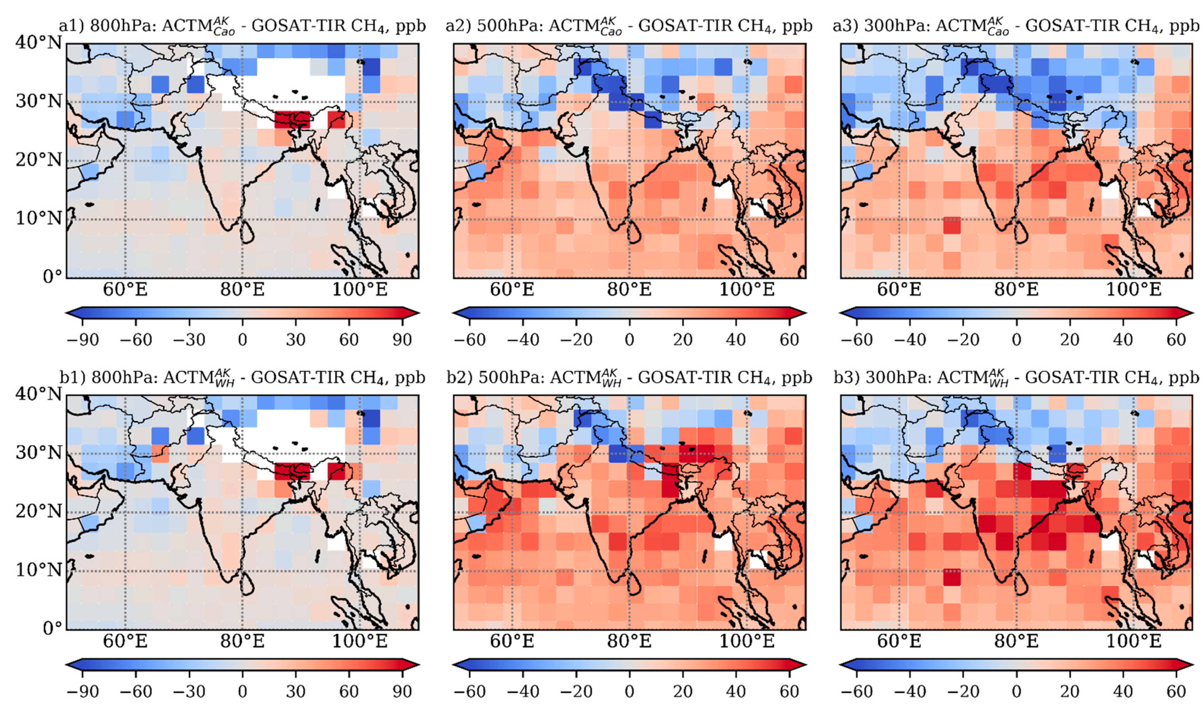
3.2. CH₄ over India Observed by GOSAT-TIR and Simulated by MIROC4-ACTM

We analyzed CH₄ distributions from GOSAT-TIR and MIROC4-ACTM regrided on the horizontal grid with a resolution of 3.0° × 3.0° and interpolated at the levels of constant pressure of 800, 500, and 300 hPa, which represent the top of the boundary layer, the free troposphere, and the upper troposphere heights of the Earth’s atmosphere, respectively. CH₄ concentrations were averaged over time for four periods: pre-monsoon April–June (AMJ), monsoon July–September (JAS), post-monsoon October–December (OND), and winter season January–March (JFM) with focus on the first three periods, because no strong difference was found between JFM and AMJ. Due to a lack of TIR CH₄ data in cloudy scenes and the influence of the complex orography of the studied area, the number of points used for averaging in each grid cell varies with height over land (Figure 4a1–a3). This is especially noticeable for the northern regions of India, because a significant part of Tibet and the Himalayas are above the level of 800 hPa (Figure 4a1). Northern India also has large sources of CH₄ with different types of emission. These two factors cause large standard deviations (SD) in CH₄ (Figure 4b1–b3). For South India and the marine regions, the SD values are much lower compared to those over the land. In the middle and upper troposphere, the perturbations from the heterogeneity of the emissions are smoothed out, the density of observation points increases; therefore, the averaging errors decrease. At a height of 300 hPa, the average SD for TIR CH₄ is approximately 25 ppb.

The density of observation points decreases with the onset of the monsoon season (Figure S1); however, it remains sufficient to detect significant changes in CH₄ concentrations even considering the relatively large SD values there. A significant increase in concentration values is noticeable, primarily in the middle and upper troposphere, which is due to the repeatedly confirmed effect of convective transport from surface sources upward. After reaching a level near the tropopause, the increased concentrations are distributed by three jets: the lateral (the cross-equatorial circulation) and transverse (flows between the arid regions of north Africa and the Near East and south Asia) monsoons, and the Walker Circulation is extended across the Pacific Ocean East [10]. The CH₄ concentration in the eastern jets is higher, because it is formed over more northern areas with larger emission. The influence of the third component (the cross-equatorial circulation) is more noticeable in the post-monsoon period (Figure S2).

TIR CH₄ retrievals are constrained to the a priori CH₄ data (panels b1–b3 of Figure 5 and Figure 6) especially in lower pressure levels due to the relatively low signal-to-noise ratio of the TIR spectra at CH₄ absorption bands [30,32]. Nevertheless, the TIR CH₄ product shows clear differences in CH₄ from the a priori values, even in the lower part of the atmosphere where sensitivity is weak (panels c1–c3 of Figure 5 and Figure 6 for AMJ and JAS, and Figures S3 and S4 for JFM and OND). These differences are mainly located in the regions with high flux uncertainty. Apparently, the a priori CH₄ simulated by NIES TM with the Emission Database for Global Atmospheric Research (EDGAR) version 32FT2000 [53] for anthropogenic CH₄, and GISS emissions [44,54] for natural CH₄ shows large negative bias in this area. This implies that an additional signal of CH₄ concentration could be captured by the GOSAT-TIR measurements.

As explained in Section 2.3, MIROC4-ACTM simulations were performed with two flux combinations reflecting different approaches for estimation of the wetland CH₄ emissions. In the pre- and post-monsoon seasons (AMJ and OND), the excess concentration due to additional emission is locked in the boundary layer (as seen from MOPITT CO) [5]; therefore, we can only detect a slight increase in concentration at the levels selected for the analysis. CH₄ simulated using both emission schemes was consistent with the GOSAT-TIR retrieval with an averaged mismatch within ±2%, the heterogeneity of which is apparently caused by transport regimes. By analogy to the CH₄ distribution from GOSAT-TIR, the increased scatter was found in modeled CH₄ over IGP, wherein the enhanced values extended up to the level of 300 hPa (see Supplementary Figures S5 and S6).

During the monsoon, the difference between emission scenarios becomes significant, as additional CH₄-rich airmass is carried to the middle and upper atmosphere (Figure 7). The large mismatch in comparison with GOSAT-TIR (panels b1–b3 of Figure 7) emphasizes the overestimation of CH₄ emission in the WH scheme. Apparently, production of CH₄ due to wetland and rice along the Ganges river in the WH scheme of the VISIT model is excessively high. More detailed flux strength estimations are in Section 3.6.

3.3. CH₄ Vertical Profiles

Figure 8 depicts seasonal mean CH₄ vertical profiles observed by GOSAT-TIR and simulated by the model for pre-monsoon (April–June) and monsoon (July–September) seasons of 2011. The variation of GOSAT-TIR sensitivity is taken into account by the implementation of the a priori profiles and AK functions (Figure 1c,e,g) to the modelled datasets (${\mathrm{ACTM}}_{\mathrm{Cao}}^{\mathrm{AK}}$ and ${\mathrm{ACTM}}_{\mathrm{WH}}^{\mathrm{AK}}$). The variabilities shown in Figure 8 are larger than GOSAT-TIR retrieval errors, derived here as the diagonal elements of the posteriori error covariance matrices based on the MAP method, which include random error components of the retrieval. Therefore, GOSAT-TIR and the model show good agreements (mismatch is inside 1-σ SD uncertainty) within both errors (natural variabilities and retrieval random errors). The vertical CH₄ profiles have a characteristic curved shape with double peak. The first peak near the surface is associated with emissions from local sources; the second one at the level of 150–200 hPa is caused by the vertical updraft [55,56]. The vertical gradient between the near-surface and upper troposphere levels increases in the direction from south-west to north-east, reflecting the increase in CH₄ surface flux intensities (Figure 2).

Monsoons cause a powerful perturbation of concentration along the entire vertical profile up to the level of the tropopause. Two southern regions (the Arabian Sea and Southern India; Figure 8a,h) are located near the entry point of Somali Jet—atmospheric masses with low CH₄ concentrations coming from the Indian Ocean [7,49]. These regions do not have significant sources of CH₄; therefore, concentrations in the vertical profiles increase with height due to transport from other regions. The third southern region (Bay of Bengal; Figure 8c) has similar properties, but at the same time, it is under the influence of transport from neighboring regions (i.e., East India, EIGP), as evidenced by a large spread near the surface.

The use of AK takes into account the relatively low vertical resolution of satellite measurements and the change in the sensitivity of the retrieval with altitude. Convolved model profiles with TIR CH₄ AK (Equation (1)) along the a priori profile smooth the model profiles to fit the GOSAT-TIR vertical resolution and reduce the mismatch at the levels where the sensitivity of satellite sensors is weak, as shown in Figure 9.The use of TIR CH₄ AK functions have a significant smoothing effect, approaching the MIROC4-ACTM model profiles to a priori so much that the difference between the calculations for the Cao and WH emission scenarios becomes barely distinguishable. This is especially visible above the level of 150 hPa, where the sensitivity of GOSAT-TIR there drops sharply, and the satellite retrievals and the AK convolved model profiles strongly follow the a priori profiles.

3.4. CH₄ Time–Altitude Variation

The monsoon anticyclone shows substantial intra-seasonal oscillations, which are connected to variable forcing from transient deep convection over the Indian subcontinent and the Bay of Bengal. This variability is typically associated with active/break cycles of the monsoon with timescales of ~10–20 days [57,58]. Significant correlations exist between outgoing longwave radiation (OLR; Figure 3a2,d2) and circulation within the monsoon region, such that the entire balanced anticyclone varies in concert with convective heating: enhanced convection leads to warmer tropospheric temperatures, stronger anticyclonic circulation, and colder lower stratospheric (and tropopause) temperatures [14]. This causes a significant heterogeneity of the flux transported upward and CH₄ concentration in the upper layers during ASMA (Figure 10).

The IGP region experiences intense agricultural activity and use of traditional biofuels. In the winter months, the IGP is often enveloped by thick fog and haze. The prevailing winds at low altitudes (surface to ~850 hPa) are northerly to northwesterly with low wind speeds (<5 m/s), and the eastern parts of the IGP are impacted by a localized area of strong subsidence in winter [59]. These conditions tend to trap the pollution at low altitudes [5].

Apparently, the a priori profiles from the NIES model show insufficient vertical transport due to inefficient convective parameterization required to simulate tracer transport under monsoon conditions (Figure 10). This problem forced the transition to a more sophisticated reanalysis JRA-25/JCDAS (Japanese 25-year Reanalysis/Climate Data Assimilation System developed by the Japan Meteorological Agency (JMA)) and the adaptation of the new parameterization as described by [55]. The GOSAT-TIR retrieval tries to compensate for such a concentration deficit in the upper troposphere.

3.5. Seasonal Variation of CH₄

The Prophet analysis model was implemented to derive mean seasonal cycles of CH₄ from GOSAT-TIR and MIROC4-ACTM for the levels of 800 and 300 hPa for 2009–2014 ignoring year-to-year variations (Figure 11). Seasonal changes are controlled primarily by meteorological parameters; therefore, the effect of the summer monsoon is most noticeable because it causes enhanced redistribution of CH₄ from lower layers to the middle and upper troposphere. As a result, in summer, the minimum CH₄ is found in the lower troposphere (800 hPa), while the maximum is in the upper part (Figure 11). The amplitude of seasonal changes is determined by the net amount of the sources; therefore, it increases from south to north from marine regions to the most densely populated areas. In the same direction, the difference between the Cao and WH fluxes increases and reached maxima in the three most northern regions (WIGP, EIGP and NEI). This inequality determines the difference between seasonal variability for host regions and spreads to the nearest neighbors. It is especially noticeable for AI and WI, where intrinsic fluxes are much smaller.

With the onset of autumn, the deep convective transport is suppressed; therefore, under the influence of the Hadley cell circulation, the slow outflow of air masses starts in the opposite south-west direction. This situation is marked by the peak of concentration at 800 hPa, which slowly moves from the northern regions (over EIGP in October) to the southern (over the Arabian Sea in late November). Despite a significant (about 50%) difference in Cao and WH emissions, the concentrations smoothed by Equation (1) differ significantly less than without implementation of the AK functions (Figure S8).

The numerical values of the seasonal cycle derived by the Prophet model (Figure 11) and averaged for individual seasons and levels of 800 and 300 hPa are presented in

Table 1. Mean and 1-σ SD uncertainty of multi-year (2009–2014) seasonal variation of CH₄ at the levels of 800 and 300 hPa for JFM, AMJ, JAS, and OND derived from GOSAT-TIR by the Prophet model as shown in Figure 11.

Regions	JFM		AMJ		JAS		OND
	800 hPa	300 hPa	800 hPa	300 hPa	800 hPa	300 hPa	800 hPa	300 hPa
Arid	–2.4 ± 10.5	–12.2 ± 3.6	–42.0 ± 12.2	–11.2 ± 10.4	24.7 ± 19.6	26.9 ± 18.0	19.7 ± 20.8	–4.3 ± 4.0
Arabian Sea	2.6 ± 5.6	–1.1 ± 1.3	–19.9 ± 14.7	–4.1 ± 4.7	–39.5 ± 13.5	–10.3 ± 8.9	56.4 ± 23.8	15.4 ± 3.9
Bay of Bengal	11.3 ± 8.2	8.3 ± 4.4	–15.5 ± 26.3	–5.8 ± 9.5	–40.4 ± 19.6	–21.8 ± 7.7	44.7 ± 15.7	19.2 ± 5.7
Central India	–3.1 ± 17.6	–12.9 ± 4.3	–51.3 ± 11.6	–13.2 ± 7.1	–10.3 ± 50.6	17.6 ± 13.9	64.6 ± 34.5	8.4 ± 12.2
Eastern India	2.4 ± 14.9	–5.8 ± 6.5	–43.8 ± 15.4	–10.9 ± 4.6	–23.3 ± 50.8	1.8 ± 12.9	64.9 ± 42.7	14.7 ± 5.9
East IGP	–25.7 ± 7.8	–11.2 ± 4.3	–4.7 ± 11.8	–4.9 ± 6.4	5.5 ± 39.7	12.7 ± 9.3	25.2 ± 34.4	3.5 ± 7.5
Northeast India	–3.3 ± 6.2	–14.1 ± 2.8	–25.8 ± 27.3	0.7 ± 6.0	–28.2 ± 50.1	9.0 ± 10.3	57.2 ± 17.7	4.6 ± 10.1
Southern India	20.2 ± 14.2	3.6 ± 6.7	–38.8 ± 34.1	–9.0 ± 7.8	–60.6 ± 27.2	–14.3 ± 10.5	82.1 ± 29.5	20.4 ± 5.8
Western India	1.4 ± 15.0	–14.4 ± 4.8	–43.7 ± 10.3	–11.0 ± 6.5	–31.6 ± 37.1	21.2 ± 13.0	73.6 ± 40.8	4.3 ± 11.5
West IGP	–24.9 ± 6.0	–11.9 ± 2.9	–20.2 ± 14.3	–10.0 ± 11.3	42.7 ± 8.5	29.5 ± 9.8	2.7 ± 26.0	–7.7 ± 5.3

. Based on these results, we found that the amplitude of seasonal changes at the level of 800 hPa was maximum for the regions in the southern and central regions of the domain (SI, WI, CI, EI), where it reached values of 100–140 ppb. At the 300 hPa level, the maximum amplitude was much lower (up to 50 ppb) in regions with high convective activity and adjacent to them (WIGP, BB, AI, WI). The seasonal cycles at the levels of 500 and 300 hPa are very similar; therefore, the free troposphere is not given in the table.

3.6. Regional CH₄ Emission Estimation

India occupies a large region of South Asia, where fewer observations limit the chance to reduce the uncertainty in the greenhouse gases (including CH₄) flux. Used in this work, the Cao and WH flux combinations for the South Asia region for the period 2009–2014 account for 65.7 ± 5.8 and 82.4 ± 7.3 Tg year⁻¹, respectively. Figure 12 shows the time variation of modelled and observed CH₄ averaged over the area of South Asia for three levels (300, 500, and 800 hPa). A significant difference in emissions appears during the monsoon, with almost equal effects in the middle and upper troposphere. Inter-annual change of trend is weak but increasing towards the top of the boundary layer (Figure 12c), where GOSAT-TIR variability can be greatly influenced due to the large spread (SD) of individual samplings (Figure 4). Another important factor is the GOSAT-TIR retrieval a priori profile derived from NIES TM with the coarse vertical grid and simplified scheme for modeling of the boundary layer height, which shows strong diurnal and seasonal variations [60]. Good consistency in the phase is found, because the ${\mathrm{ACTM}}_{\mathrm{Cao}}^{\mathrm{AK}}$, and ${\mathrm{ACTM}}_{\mathrm{WH}}^{\mathrm{AK}}$ are overlapped during non-monsoon periods, and concentration mismatch is strongly associated with the flux difference.

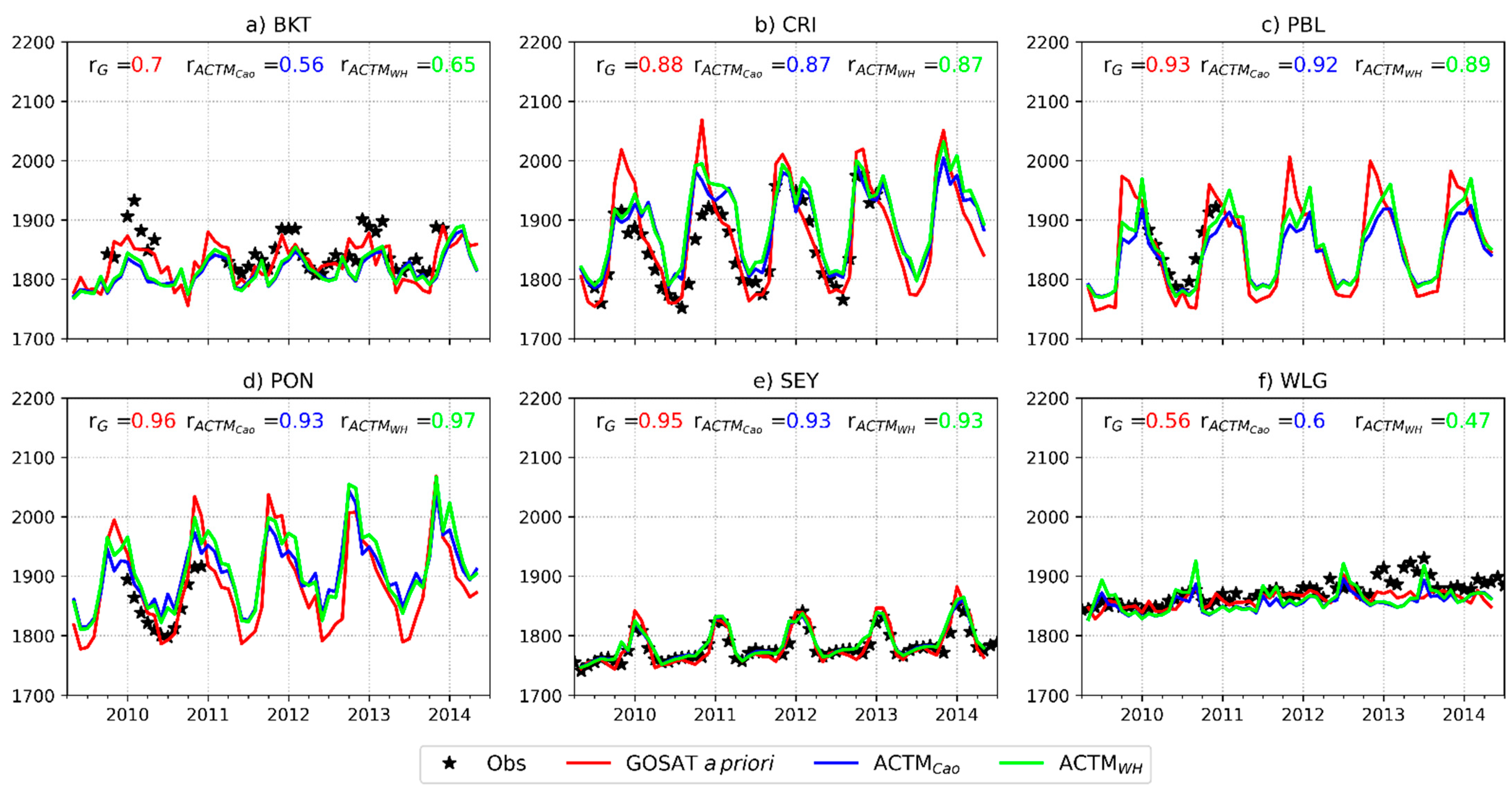
3.7. Comparison with Ground Observations

GOSAT-TIR measurements are less sensitive to CH₄ concentrations near the surface, which makes it difficult to discuss based on direct comparison with ground-based observations. However, such comparisons are useful for evaluating the MIROC4-ACTM model and a priori distributions. The number of ground observation stations in India is limited; therefore, we also included observations from the surrounded regions for an overall assessment of the comparison results.

Figure 13 shows a comparison with surface observations over Bukit Kototabang, Indonesia (BKT—0.2° S, 100.3° E, 845 m a.s.l.), Cape Rama (CRI—15.1° N, 73.8° E, 60 m a.s.l.), Seychelles (SEY—4.7° N, 55.2° E, 3 m a.s.l.), Mt. Waliguan, China (WLG—36.3° N, 100.9° E, 3810 m a.s.l.) provided by World Data Centre for Greenhouse Gases (WDCGG). For observations performed by Laboratoire des Sciences du Climat et de l’Environnement (LSCE) over the Pondicherry (PON) station (12.0° N, 79.9° E, 20 m a.s.l), and the Port Blair (PBL) station (11.7° N, 92.8° E, 20 m a.s.l.), only mean seasonal cycle data are available. Therefore, for these sites, the concentration values were adjusted using the average concentrations. For comparison, the surface values from the GOSAT-TIR and MIROC4-ACTM CH₄ profiles within a radius of 2.5° from the observation site coordinates were selected and monthly averaged.

Selected sites represent a diverse variety of CH₄, which has different interpretations. The remote marine site (SEY) and high-mountain sites (WLG) are influenced by large-scale processes. Low bias (~5 ppb) and SD (~20 ppb) confirm the ability to reproduce the global CH₄ budget. The BKT, CRI, PBL, and PON sites represent coastal regions with variable local meteorology controlling CH₄. Judging by the correlation coefficient (r), the performance of the model is quite high (r = 0.9), although it decreases in mountainous and densely populated areas (r = 0.6).

4. Discussion

Analysis of CH₄ from GOSAT-TIR and MIROC4-ACTM has several important aspects underlining GOSAT-TIR retrieval itself, but also its implementation on studies over India. Despite essential progress, the development of satellite methods for studying atmospheric CH₄ is obstructed by a few limitations. The launch rate of new orbital instruments is significantly ahead of the development of a ground-based and aircraft measurement network for their validation. Due to the scarcity of suitable aircraft observations over India, validation of GOSAT-TIR profiles cannot cover all seasons and land regions studied in this work.

In comparison with AIRS satellite observations [61], the finer vertical resolution of GOSAT-TIR allows capturing more detailed features in CH₄ vertical profiles and therefore more prominent patterns related to different regions and seasons. The significant difference in the CH₄ profile gradient, and its seasonal variability (winter and summer) between a priori and the MIROC4-ACTM model, was revealed in the UT/LS zone (150–200 hPa). During monsoon season, daily variation in a priori profiles is also found in the middle troposphere. While [8] mainly used the model simulations to understand the vertical transport (after validating the model using GOSAT-SWIR measurements), we showed the seasonal evolution of transport and emissions on CH₄ at different layers of the troposphere using both the model and GOSAT-TIR measurements. Unlike work conducted by [7], we found a strong difference between seasons in the middle and upper troposphere caused by variability in atmospheric circulation and vertical convection.

A priori profiles play an essential role in processing a satellite signal, especially for the CH₄, which has a significant change in a lifetime with altitude. The choice of such a profile (usually provided by model calculations) is critical because of small DOF in observed spectra; the retrieval algorithms cannot overcome large errors in input a priori data. The TransCom-CH₄ experiment [44] showed a significant scatter between the participated models, including the NIES model later selected for calculating the GOSAT-TIR a priori profile (described in Section 2.2). In this study, the difference in the CH₄ profile gradient, its seasonal variability (winter and summer) between a priori and the MIROC4-ACTM model was revealed in the UT/LS zone (levels of 150–20 hPa). This emphasizes the difference in vertical resolution and reanalyzes for the calculation of vertical profiles (described in Section 2.3 and Section 2.4). However, the reason for the misfits (GOSAT-TIR a priori vs. ACTM) is difficult to reconcile without additional studies with the use of custom a priori profiles in retrieval.

In the case of long-term projects, the updating of a priori data in accordance with the current progress becomes important. From the moment of the GOSAT launch, the calculations of a priori profiles are carried out according to the same scheme. This is important for the long-term consistency of the TIR CH₄ product but does not take into account the recent improvements (e.g., new reanalysis data, higher vertical resolution, and convective parameterizations) implemented in MIROC4-ACTM [36], as well as further understanding of the CH₄ budget [62]. The release of a new version of retrieval algorithms designed to improve and update satellite products is not regular; therefore, perhaps, for further progress, the retrieval algorithms may use some custom a priori information for checking initial results. Therefore, this will require greater transparency of technical information from satellite projects and significant optimization of retrieval calculations, because such tasks require large computational resources. However, this a priori profile issue remains hidden (but no less relevant) in the field of the main efforts of the scientific community working with XCH₄ derived from the SWIR band, apart from applying the a priori correction.

Another issue of concern, as we found, was the implementation of AK functions. Without AK processing, mean MIROC4-ACTM and GOSAT-TIR mismatches were within 50 ppb, except for the level of 150 hPa and upward, where the GOSAT-TIR sensitivity becomes very low. Convolved model profiles with retrieval a priori and AK functions reduce the mismatch to below uncertainty, making the influence of the a priori profiles too large.

The lack of reliable data for the estimation of regional CH₄ budgets can be mitigated by TIR CH₄. Relying on our comparison (Figure 12), we suggest the Cao flux combination with the annual mean South Asian emission of 65.7 ± 5.8 Tg year⁻¹ for the period 2009–2014 as more plausible. This confirms the assessment made by [63], indicating that the EDGAR inventory (version 4.2FT2010) with a value of 73.3–83.2 Tg year⁻¹ overestimated the South Asia regional emission by 10–15 Tg year⁻¹. A significant part of the extra fluxes was concentrated in a few relatively small regions in Northern India (Figure 2). However, our best estimate emission of 51.2 ± 4.6 Tg year⁻¹ over India is much greater than the 19.6–24.3 Tg year⁻¹ estimated by [6], who combined in situ data of different time coverage and SWIR CH₄ retrievals in the trajectory-based modelling framework, but is in good agreement with the mean emissions of 48.9 Tg year⁻¹ calculated by [40]. Simulation with two scenarios showed that during the monsoon, significant CH₄ amounts due to extra fluxes can quickly propagate to the UT/LS zone and not be detected by ground-based measurements.

Overall, the MIROC4-ACTM simulations of CH₄ in the Indian regions are consistent with the GOSAT-TIR samplings, in terms of seasonality and global variability. Although we found noticeable error in the model data in phase and amplitude at the end of the summer–fall period, the model performance in CH₄ transport in the troposphere and the lower stratosphere was improved due to the use of MIROC4.0 as the meteorological model. Inconsistencies seen in the model-observation comparisons provide opportunities for further flux optimization with inverse modeling methods. More insights are expected after the extension of the released data period of the TIR CH₄ product.

5. Conclusions

CH₄ from GOSAT-TIR observations and MIROC4-ACTM simulations, sampled at the location and time of the satellite overpass, were analyzed over India and surrounding oceanic regions for the period 2009–2014. The area of our analysis was subdivided into eight land and two ocean regions. We studied the seasonal variation of CH₄ at the atmospheric levels of 800 and 300 hPa over Indian regions and found a large time–spatial inhomogeneity. The major factors controlling it included change in local emission strength, variability in atmospheric circulation, and vertical convection caused by the Asian summer monsoon.

GOSAT-TIR observations are less affected by cloud conditions and could be performed during night; therefore, suitable data coverage and density (10–200 observation samples per 3.0° × 3.0° grid cell per month) are obtained to study CH₄ over India. By capturing signals from the top of the atmospheric boundary layer (except for high mountain regions) up to UT/LS, detailed horizontal and vertical features of CH₄ are revealed. Differences from the a priori values suggest that the CH₄ concentration signal was captured even in the lower part of the troposphere, where sensitivity of the GOSAT-TIR sensor is relatively weak compared to the middle and upper troposphere. The mean TIR CH₄ model mismatch was within 50 ppb, except for the altitude range above 150 hPa, where the sensitivity of GOSAT-TIR observations becomes very low.

The MIROC4-ACTM simulations were conducted using two surface fluxes optimized by the inverse analysis describing different approaches of modelling CH₄ emissions from wetlands. Among these scenarios, the Cao scheme seems to be more balanced than WH for individual regions and the whole of South Asia during the monsoon season. In the other periods, no strong difference was found. The flux difference is effective to show the strength of surface concentration propagation to the middle and upper troposphere. Using comparison with GOSAT-TIR, we identified the annual mean emission for the period 2009–2014 for South Asia and India as of 65.7 ± 5.8 and 51.2 ± 4.6 Tg year⁻¹, respectively.

Despite substantial improvements and testing in various validation projects [44,63], CTMs are still considered as an insufficiently reliable method of studies. However, for many regions/cases, it is only one available source of new knowledge, that would identify general trends, indicate optimal methods of development, and motivate the making of accurate field/aircraft measurements. Our results suggest that an additional comparison with aircraft observations is necessary to analyze the GOSAT-TIR and MIROC4-ACTM mismatch found above the level of 150 hPa. Furthermore, the selection of the a priori model for satellite data retrieval could play a significant role and should be addressed in the developments of future retrieval systems.

References

1. Patra, P.K.; Canadell, J.G.; Houghton, R.A.; Piao, S.L.; Oh, N.-H.; Ciais, P.; Manjunath, K.R.; Chhabra, A.; Wang, T.; Bhattacharya, T.; et al. The carbon budget of South Asia. Biogeosciences 2013, 10, 513–527. [Google Scholar] [CrossRef] [Green Version]
2. Akimoto, H. Global Air Quality and Pollution. Science 2003, 302, 1716–1719. [Google Scholar] [CrossRef] [PubMed] [Green Version]
3. Ohara, T.; Akimoto, H.; Kurokawa, J.; Horii, N.; Yamaji, K.; Yan, X.; Hayasaka, T. An Asian emission inventory of anthropogenic emission sources for the period 1980–2020. Atmos. Chem. Phys. 2007, 7, 4419–4444. [Google Scholar] [CrossRef] [Green Version]
4. Janssens-Maenhout, G.; Crippa, M.; Guizzardi, D.; Muntean, M.; Schaaf, E.; Dentener, F.; Bergamaschi, P.; Pagliari, V.; Olivier, J.G.J.; Peters, J.A.H.W.; et al. EDGAR v4.3.2 Global Atlas of the three major greenhouse gas emissions for the period 1970–2012. Earth Syst. Sci. Data 2019, 11, 959–1002. [Google Scholar] [CrossRef] [Green Version]
5. Kar, J.; Deeter, M.N.; Fishman, J.; Liu, Z.; Omar, A.; Creilson, J.K.; Trepte, C.R.; Vaughan, M.A.; Winker, D.M. Wintertime pollution over the Eastern Indo-Gangetic Plains as observed from MOPITT, CALIPSO and tropospheric ozone residual data. Atmos. Chem. Phys. 2010, 10, 12273–12283. [Google Scholar] [CrossRef] [Green Version]
6. Ganesan, A.L.; Rigby, M.; Lunt, M.F.; Parker, R.J.; Boesch, H.; Goulding, N.; Umezawa, T.; Zahn, A.; Chatterjee, A.; Prinn, R.G.; et al. Atmospheric observations show accurate reporting and little growth in India’s methane emissions. Nat. Commun. 2017, 8, 1–7. [Google Scholar] [CrossRef] [Green Version]
7. Guha, T.; Tiwari, Y.K.; Valsala, V.; Lin, X.; Ramonet, M.; Mahajan, A.; Datye, A.; Kumar, K.R. What controls the atmospheric methane seasonal variability over India? Atmos. Environ. 2018, 175, 83–91. [Google Scholar] [CrossRef] [Green Version]
8. Chandra, N.; Hayashida, S.; Saeki, T.; Patra, P.K. What controls the seasonal cycle of columnar methane observed by GOSAT over different regions in India? Atmos. Chem. Phys. 2017, 17, 12633–12643. [Google Scholar] [CrossRef] [Green Version]
9. Lin, X.; Ciais, P.; Bousquet, P.; Ramonet, M.; Yin, Y.; Balkanski, Y.; Cozic, A.; Delmotte, M.; Evangeliou, N.; Indira, N.K.; et al. Simulating CH4 and CO2 over South and East Asia using the zoomed chemistry transport model LMDz-INCA. Atmos. Chem. Phys. 2018, 18, 9475–9497. [Google Scholar] [CrossRef] [Green Version]
10. Webster, P.J.; Magaña, V.O.; Palmer, T.N.; Shukla, J.; Tomas, R.A.; Yanai, M.; Yasunari, T. Monsoons: Processes, predictability, and the prospects for prediction. J. Geophys. Res. Ocean. 1998, 103, 14451–14510. [Google Scholar] [CrossRef]
11. Fleitmann, D.; Burns, S.J.; Mangini, A.; Mudelsee, M.; Kramers, J.; Villa, I.; Neff, U.; Al-Subbary, A.A.; Buettner, A.; Hippler, D.; et al. Holocene ITCZ and Indian monsoon dynamics recorded in stalagmites from Oman and Yemen (Socotra). Quat. Sci. Rev. 2007, 26, 170–188. [Google Scholar] [CrossRef]
12. Fu, R.; Hu, Y.; Wright, J.S.; Jiang, J.H.; Dickinson, R.E.; Chen, M.; Filipiak, M.; Read, W.G.; Waters, J.W.; Wu, D.L. Short circuit of water vapor and polluted air to the global stratosphere by convective transport over the Tibetan Plateau. Proc. Natl. Acad. Sci. USA 2006, 103, 5664–5669. [Google Scholar] [CrossRef] [Green Version]
13. Randel, W.J.; Park, M.; Emmons, L.; Kinnison, D.; Bernath, P.; Walker, K.A.; Boone, C.; Pumphrey, H. Asian monsoon transport of pollution to the stratosphere. Science 2010, 328, 611–613. [Google Scholar] [CrossRef] [Green Version]
14. Randel, W.J.; Park, M. Deep convective influence on the Asian summer monsoon anticyclone and associated tracer variability observed with Atmospheric Infrared Sounder (AIRS). J. Geophys. Res. Atmos. 2006, 111, 1–13. [Google Scholar] [CrossRef]
15. Xiong, X.; Houweling, S.; Wei, J.; Maddy, E.; Sun, F.; Barnet, C. Methane plume over south Asia during the monsoon season: Satellite observation and model simulation. Atmos. Chem. Phys. 2009, 9, 783–794. [Google Scholar] [CrossRef] [Green Version]
16. Garny, H.; Randel, W.J. Transport pathways from the Asian monsoon anticyclone to the stratosphere. Atmos. Chem. Phys. 2016, 16, 2703–2718. [Google Scholar] [CrossRef] [Green Version]
17. Park, M.; Randel, W.J.; Kinnison, D.E.; Garcia, R.R.; Choi, W. Seasonal variation of methane, water vapor, and nitrogen oxides near the tropopause: Satellite observations and model simulations. J. Geophys. Res. Atmos. 2004. [Google Scholar] [CrossRef] [Green Version]
18. Park, M.; Randel, W.J.; Emmons, L.K.; Bernath, P.F.; Walker, K.A.; Boone, C.D. Chemical isolation in the Asian monsoon anticyclone observed in Atmospheric Chemistry Experiment (ACE-FTS) data. Atmos. Chem. Phys. 2008, 8, 757–764. [Google Scholar] [CrossRef] [Green Version]
19. Butz, A.; Hasekamp, O.P.; Frankenberg, C.; Vidot, J.; Aben, I. CH4 retrievals from space-based solar backscatter measurements: Performance evaluation against simulated aerosol and cirrus loaded scenes. J. Geophys. Res. Atmos. 2010. [Google Scholar] [CrossRef] [Green Version]
20. Parker, R.; Boesch, H.; Cogan, A.; Fraser, A.; Feng, L.; Palmer, P.I.; Messerschmidt, J.; Deutscher, N.; Griffith, D.W.T.; Notholt, J.; et al. Methane observations from the Greenhouse Gases Observing SATellite: Comparison to ground-based TCCON data and model calculations. Geophys. Res. Lett. 2011, 38. [Google Scholar] [CrossRef] [Green Version]
21. Yoshida, Y.; Kikuchi, N.; Morino, I.; Uchino, O.; Oshchepkov, S.; Bril, A.; Saeki, T.; Schutgens, N.; Toon, G.C.; Wunch, D.; et al. Improvement of the retrieval algorithm for GOSAT SWIR XCO2 and XCH4 and their validation using TCCON data. Atmos. Meas. Tech. Discuss. 2013, 6, 949–988. [Google Scholar]
22. Saitoh, N.; Kimoto, S.; Sugimura, R.; Imasu, R.; Kawakami, S.; Shiomi, K.; Kuze, A.; Machida, T.; Sawa, Y.; Matsueda, H. Algorithm update of the GOSAT/TANSO-FTS thermal infrared CO2 product (version 1) and validation of the UTLS CO2 data using CONTRAIL measurements. Atmos. Meas. Tech. 2016, 9, 2119–2134. [Google Scholar] [CrossRef] [Green Version]
23. De Lange, A.; Landgraf, J. Methane profiles from GOSAT thermal infrared spectra. Atmos. Meas. Tech. 2018, 11, 3815–3828. [Google Scholar] [CrossRef] [Green Version]
24. Ricaud, P.; Sic, B.; El Amraoui, L.; Attié, J.L.; Zbinden, R.; Huszar, P.; Szopa, S.; Parmentier, J.; Jaidan, N.; Michou, M.; et al. Impact of the Asian monsoon anticyclone on the variability of mid-to-upper tropospheric methane above the Mediterranean Basin. Atmos. Chem. Phys. 2014, 14, 11427–11446. [Google Scholar] [CrossRef] [Green Version]
25. Rodgers, C.D. Inverse Methods for Atmospheric Sounding: Theory and Practice, Series on Atmospheric, Oceanic and Planetary Physics—Volume 2; World Scientific Publishing: Singapore, 2000. [Google Scholar]
26. Cooper, M.; Martin, R.; Henze, D.; Jones, D. Effects of a priori profile shape assumptions oncomparisons between satellite NO2 columns and model simulations. Atmos. Chem. Phys. 2020, 20, 7231–7241. [Google Scholar] [CrossRef]
27. Yokota, T.; Yoshida, Y.; Eguchi, N.; Ota, Y.; Tanaka, T.; Watanabe, H.; Maksyutov, S. Global concentrations of CO2 and CH4 retrieved from GOSAT: First preliminary results. Sci. Online Lett. Atmos. 2009. [Google Scholar] [CrossRef] [Green Version]
28. Kuze, A.; Suto, H.; Nakajima, M.; Hamazaki, T. Thermal and near infrared sensor for carbon observation Fourier-transform spectrometer on the Greenhouse Gases Observing Satellite for greenhouse gases monitoring. Appl. Opt. 2009, 48, 6716–6733. [Google Scholar] [CrossRef] [PubMed]
29. Kuze, A.; Suto, H.; Shiomi, K.; Urabe, T.; Nakajima, M.; Yoshida, J.; Kawashima, T.; Yamamoto, Y.; Kataoka, F.; Buijs, H. Level 1 algorithms for TANSO on GOSAT: Processing and on-orbit calibrations. Atmos. Meas. Tech. 2012. [Google Scholar] [CrossRef] [Green Version]
30. Saitoh, N.; Touno, M.; Hayashida, S.; Imasu, R.; Shiomi, K.; Yokota, T.; Yoshida, Y.; Machida, T.; Matsueda, H.; Sawa, Y. Comparisons between XCH4 from GOSAT Shortwave and Thermal Infrared Spectra and Aircraft CH4 Measurements over Guam. Sola 2012, 8, 145–149. [Google Scholar] [CrossRef]
31. Holl, G.; Walker, K.A.; Conway, S.; Saitoh, N.; Boone, C.D.; Strong, K.; Drummond, J.R. Methane cross-validation between three Fourier transform spectrometers: SCISAT ACE-FTS, GOSAT TANSO-FTS, and ground-based FTS measurements in the Canadian high Arctic. Atmos. Meas. Tech. 2016, 9, 1961–1980. [Google Scholar] [CrossRef] [Green Version]
32. Zou, M.; Xiong, X.; Saitoh, N.; Warner, J.; Zhang, Y.; Chen, L.; Weng, F.; Fan, M. Satellite observation of atmospheric methane: Intercomparison between AIRS and GOSAT TANSO-FTS retrievals. Atmos. Meas. Tech. 2016, 9, 3567–3576. [Google Scholar] [CrossRef] [Green Version]
33. Olsen, K.S.; Strong, K.; Walker, K.A.; Boone, C.D.; Raspollini, P.; Plieninger, J.; Bader, W.; Conway, S.; Grutter, M.; Hannigan, J.W.; et al. Comparison of the GOSAT TANSO-FTS TIR CH volume mixing ratio vertical profiles with those measured by ACE-FTS, ESA MIPAS, IMK-IAA MIPAS, and 16 NDACC stations. Atmos. Meas. Tech. 2017, 10, 3697–3718. [Google Scholar] [CrossRef] [Green Version]
34. Saeki, T.; Saito, R.; Belikov, D.; Maksyutov, S. Global high-resolution simulations of CO2 and CH4 using a NIES transport model to produce a priori concentrations for use in satellite data retrievals. Geosci. Model Dev. 2013, 6, 81–100. [Google Scholar] [CrossRef] [Green Version]
35. Watanabe, S.; Miura, H.; Sekiguchi, M.; Nagashima, T.; Sudo, K.; Emori, S.; Kawamiya, M. Development of an Atmospheric General Circulation Model for Integrated Earth System Modeling on the Earth Simulator. J. Earth Simulator 2008, 9, 27–35. [Google Scholar]
36. Patra, P.K.; Takigawa, M.; Watanabe, S.; Chandra, N.; Ishijima, K.; Yamashita, Y. Improved chemical tracer simulation by MIROC4.0-based atmospheric chemistry-transport model (MIROC4-ACTM). Sci. Online Lett. Atmos. 2018. [Google Scholar] [CrossRef] [Green Version]
37. Kobayashi, S.; Ota, Y.; Harada, Y.; Ebita, A.; Moriya, M.; Onoda, H.; Onogi, K.; Kamahori, H.; Kobayashi, C.; Endo, H.; et al. The JRA-55 reanalysis: General specifications and basic characteristics. J. Meteorol. Soc. Jpn. 2015, 93, 5–48. [Google Scholar] [CrossRef] [Green Version]
38. Spivakovsky, C.M.; Logan, J.A.; Montzka, S.A.; Balkanski, Y.J.; Foreman-Fowler, M.; Jones, D.B.A.; Horowitz, L.W.; Fusco, A.C.; Brenninkmeijer, C.A.M.; Prather, M.J.; et al. Three-dimensional climatological distribution of tropospheric OH: Update and evaluation. J. Geophys. Res. Atmos. 2000. [Google Scholar] [CrossRef]
39. Patra, P.K.; Krol, M.C.; Montzka, S.A.; Arnold, T.; Atlas, E.L.; Lintner, B.R.; Stephens, B.B.; Xiang, B.; Elkins, J.W.; Fraser, P.J.; et al. Observational evidence for interhemispheric hydroxyl-radical parity. Nature 2014, 513, 219–223. [Google Scholar] [CrossRef]
40. Chandra, N.; Patra, P.K.; Bisht, J.S.H.; Ito, A.; Morimoto, S.; Janssens-Maenhout, G.; Umezawa, T.; Fujita, R.; Takigawa, M.; Watanabe, S.; et al. Emissions from the oil and gas sectors, coal mining and ruminant farming drive methane growth over the past three decades. J Meteorol. Soc. Jpn. 2021. [Google Scholar] [CrossRef]
41. Cao, M.; Marshall, S.; Gregson, K. Global carbon exchange and methane emissions from natural wetlands: Application of a process-based model. J. Geophys. Res. Atmos. 1996. [Google Scholar] [CrossRef] [Green Version]
42. Walter, B.P.; Heimann, M.; Matthews, E. Modeling modern methane emissions from natural wetlands Model description and results. J. Geophys. Res. Atmos. 2001. [Google Scholar] [CrossRef] [Green Version]
43. Van Der Werf, G.R.; Randerson, J.T.; Giglio, L.; Van Leeuwen, T.T.; Chen, Y.; Rogers, B.M.; Mu, M.; Van Marle, M.J.E.; Morton, D.C.; Collatz, G.J.; et al. Global fire emissions estimates during 1997–2016. Earth Syst. Sci. Data 2017, 9, 697–720. [Google Scholar] [CrossRef] [Green Version]
44. Patra, P.K.; Houweling, S.; Krol, M.; Bousquet, P.; Belikov, D.; Bergmann, D.; Bian, H.; Cameron-Smith, P.; Chipperfield, M.P.; Corbin, K.; et al. TransCom model simulations of CH4 and related species: Linking transport, surface flux and chemical loss with CH4 variability in the troposphere and lower stratosphere. Atmos. Chem. Phys. 2011, 11, 12813–12837. [Google Scholar] [CrossRef] [Green Version]
45. Ito, A.; Tohjima, Y.; Saito, T.; Umezawa, T.; Hajima, T.; Hirata, R.; Saito, M.; Terao, Y. Methane budget of East Asia, 1990–2015: A bottom-up evaluation. Sci. Total Environ. 2019, 676, 40–52. [Google Scholar] [CrossRef]
46. Ito, A. Methane emission from pan-Arctic natural wetlands estimated using a process-based model, 1901–2016. Polar Sci. 2019, 21, 26–36. [Google Scholar] [CrossRef] [Green Version]
47. Taylor, S.J.; Letham, B. Forecasting at Scale. Am. Stat. 2018. [Google Scholar] [CrossRef]
48. Belikov, D.; Arshinov, M.; Belan, B.; Davydov, D.; Fofonov, A.; Sasakawa, M.; Machida, T. Analysis of the diurnal, weekly, and seasonal cycles and annual trends in atmospheric CO2 and CH4 at tower network in Siberia from 2005 to 2016. Atmosphere 2019, 10, 689. [Google Scholar] [CrossRef] [Green Version]
49. Findlater, J. A major low-level air current near the Indian Ocean during the northern summer. Q. J. R. Meteorol. Soc. 1969. [Google Scholar] [CrossRef]
50. Metya, A.; Datye, A.; Chakraborty, S.; Tiwari, Y.K.; Sarma, D.; Bora, A.; Gogoi, N. Diurnal and seasonal variability of CO2 and CH4 concentration in a semi-urban environment of western India. Sci. Rep. 2021, 11, 2931. [Google Scholar] [CrossRef]
51. Devasthale, A.; Fueglistaler, S. A climatological perspective of deep convection penetrating the TTL during the Indian summer monsoon from the AVHRR and MODIS instruments. Atmos. Chem. Phys. 2010, 10, 4573–4582. [Google Scholar] [CrossRef] [Green Version]
52. Bergman, J.W.; Fierli, F.; Jensen, E.J.; Honomichl, S.; Pan, L.L. Boundary layer sources for the asian anticyclone: Regional contributions to a vertical conduit. J. Geophys. Res. Atmos. 2013, 118, 2560–2575. [Google Scholar] [CrossRef]
53. Olivier, J.G.J.; Berdowski, J.J.M. Global Emissions Sources and Sinks. In The Climate System; A.A. Balkema Publishers/Swets and Zeitlinger Publishers: Lisse, The Netherlands, 2001; pp. 33–78. [Google Scholar]
54. Fung, I. Three-dimensional model synthesis of the global methane cycle. J. Geophys. Res. 1991. [Google Scholar] [CrossRef]
55. Belikov, D.A.; Maksyutov, S.; Krol, M.; Fraser, A.; Rigby, M.; Bian, H.; Agusti-Panareda, A.; Bergmann, D.; Bousquet, P.; Cameron-Smith, P.; et al. Off-line algorithm for calculation of vertical tracer transport in the troposphere due to deep convection. Atmos. Chem. Phys. 2013, 13, 1093–1114. [Google Scholar] [CrossRef] [Green Version]
56. Saito, R.; Patra, P.K.; Sweeney, C.; Machida, T.; Krol, M.; Houweling, S.; Bousquet, P.; Agusti-Panareda, A.; Belikov, D.; Bergmann, D.; et al. TransCom model simulations of methane: Comparison of vertical profiles with aircraft measurements. J. Geophys. Res. Atmos. 2013, 118, 3891–3904. [Google Scholar] [CrossRef]
57. Krishnamurti, T.N.; Ardanuy, P. The 10- to 20-day westward propagating mode and ‘Breaks in the Monsoons’. Tellus 1980. [Google Scholar] [CrossRef]
58. Tiwari, Y.K.; Guha, T.; Valsala, V.; Lopez, A.S.; Cuevas, C.; Fernandez, R.P.; Mahajan, A.S. Understanding atmospheric methane sub-seasonal variability over India. Atmos. Environ. 2020, 223, 117206. [Google Scholar] [CrossRef]
59. Dey, S.; Di Girolamo, L. A climatology of aerosol optical and microphysical properties over the Indian subcontinent from 9 years (2000–2008) of Multiangle Imaging Spectroradiometer (MISR) data. J. Geophys. Res. Atmos. 2010, 115, 1–22. [Google Scholar] [CrossRef] [Green Version]
60. Kavitha, M.; Nair, P.R.; Girach, I.A.; Aneesh, S.; Sijikumar, S.; Renju, R. Diurnal and seasonal variations in surface methane at a tropical coastal station: Role of mesoscale meteorology. Sci. Total Environ. 2018, 631–632, 1472–1485. [Google Scholar] [CrossRef]
61. Kavitha, M.; Nair, P.R. Satellite-retrieved vertical profiles of methane over the Indian region: Impact of synoptic-scale meteorology. Int. J. Remote Sens. 2019, 40, 5585–5616. [Google Scholar] [CrossRef]
62. Saunois, M.R.; Stavert, A.; Poulter, B.; Bousquet, P.G.; Canadell, J.B.; Jackson, R.A.; Raymond, P.J.; Dlugokencky, E.; Houweling, S.K.; Patra, P.; et al. The global methane budget 2000–2017. Earth Syst. Sci. Data 2020, 12, 1561–1623. [Google Scholar] [CrossRef]
63. Patra, P.K.; Saeki, T.; Dlugokencky, E.J.; Ishijima, K.; Umezawa, T.; Ito, A.; Aoki, S.; Morimoto, S.; Kort, E.A.; Crotwell, A.; et al. Regional methane emission estimation based on observed atmospheric concentrations (2002–2012). J. Meteorol. Soc. Jpn. 2016, 94, 91–113. [Google Scholar] [CrossRef] [Green Version]
Figure 1. The map of the regional divisions for the analysis (a), depicted by unicolor boxes with the name abbreviations defined in Section 2.1. The black lines in-land show major rivers in the plot domain; the human settlements along the rivers are major sources of CH4. The TIR CH4 a priori with 1-σ SD uncertainty (red line with error bars) and TIR CH4 profile with the retrieval error (blue line with shaded area) are shown in panels (b,d,f), and the 22 AK functions corresponding to the 22 retrieval layers are in panels (c,e,g). Data in panels (bg) are shown for the regions Northeast India, Southern India, and the Bay of Bengal, averaged over the period July–September 2011.
Remotesensing 13 01677 g001
Figure 2. The surface CH4 fluxes (g-CH4/m2/month) used for MIROC4-ACTM simulation: (a1,a2) from Cao scheme, (b1,b2) difference between schemes (WH—Cao). Panels (a1,b1), and (a2,b2) are for AMJ and JAS, respectively.
Remotesensing 13 01677 g002
Figure 3. Wind vectors for the JFM (panels a1a3), AMJ (b1b3), JAS (c1c3), and OND (d1d3) months of 2010 from the MIROC4-ACTM simulations are shown. Please note different vector scales for the levels of 800 (panels a1d1), 500 (a2d2), and 200 hPa (a3d3), respectively. At the background: left panels (a1d1) show monthly surface pressure (0.9950 sigma level) from the National Centers for Environmental Prediction (NCEP) reanalysis for 2011 (http://www.esrl.noaa.gov/psd/data/gridded/data.ncep.reanalysis.derived.html accessed on 27 March 2021), central panels (a2d2) show monthly long term mean interpolated outgoing longwave radiation (OLR) from the National Oceanic and Atmospheric Administration (NOAA) for 2011 (https://www.esrl.noaa.gov/psd/data/gridded/data.interp_OLR.html accessed on 27 March 2021), and the right panels (a3d3) show daily mean cloud top pressure (hPa) from the level-3 MODIS atmosphere daily global product (v6.1) downloaded from the Giovanni online data system (Acker and Leptoukh, 2007) for 2011.
Remotesensing 13 01677 g003
Figure 4. Latitude–longitude distributions of TIR CH4 properties at the levels of 800, 500, and 300 hPa (the left, middle, and right panels, respectively) for the season AMJ 2011. The top (a1a3) and bottom rows show TIR CH4 observation points numbers, and TIR CH4 1-σ SD (b1b3), respectively.
Remotesensing 13 01677 g004
Figure 5. Latitude–longitude distributions of CH4 at the levels of 800, 500, and 300 hPa (the left, middle, and right panels, respectively) observed by GOSAT-TIR for the season AMJ 2011. The top (a1a3), middle (b1b3) and bottom (c1c3) rows show TIR CH4, TIR CH4 a priori, and difference between the TIR CH4 and a priori distributions, respectively.
Remotesensing 13 01677 g005
Figure 6. Same as Figure 5, but for JAS 2011.
Remotesensing 13 01677 g006
Figure 7. Latitude–longitude difference in CH4 distributions simulated by MIROC4-ACTM and observed by GOSAT-TIR at the levels of 800, 500, and 300 hPa (the left, middle, and right panels, respectively) for JAS 2011. The top row (a1a3) and bottom row (b1b3) show the difference in CH4 between GOSAT-TIR, and ACTM Cao and ACTM WH , respectively.
Remotesensing 13 01677 g007
Figure 8. Seasonal mean CH4 vertical profiles for pre-monsoon (April–June) and monsoon (July–September) of 2011 are shown in the left and right part of each panels (bk) for the different regions as depicted in the central map (a). Black line with error bars shows the GOSAT-TIR data with 1-σ SD uncertainty. Blue and red lines with shaded areas correspond to the ACTM Cao AK and ACTM WH AK data with 1-σ SD uncertainty, respectively.
Remotesensing 13 01677 g008
Figure 9. Seasonal mean CH4 vertical profiles (ae) for winter (January–March) and (fj) monsoon (July–September) periods of 2011 are shown for the selected regions. Black line shows the GOSAT-TIR a priori data. Green and magenta lines with shaded areas correspond to the ACTM Cao and ACTM WH data with 1-σ SD uncertainty, respectively. Red and blue lines represent the CH4 from ACTM Cao AK and ACTM WH AK smoothed with the AK functions implementation.
Remotesensing 13 01677 g009
Figure 10. Time–altitude cross-section of CH4 from GOSAT-TIR retrieval, GOSAT-TIR a priori, and ACTM Cao AK (the left, middle, and right panels, respectively) for the Arabian Sea, Arid, and EIGP regions (for all regions please see Figure S7). Note that the profiles are shown for the tropospheric altitudes because the GOSAT-TIR retrieval system is not sensitive to the stratospheric altitudes (see Figure 8 and the associated text).
Remotesensing 13 01677 g010
Figure 11. Multi-year (2009–2014) seasonal variation of CH4 (right y-axis) derived by implementation of the Prophet model for levels of 800 (red lines) and 300 hPa (blue lines) over considered regions from GOSAT-TIR (solid line), ACTM Cao AK (dashed line), and ACTM WH AK (dotted line), respectively. At the background, bar plots represent Cao (dark grey) and WH (light grey) CH4 fluxes (left y-axis), respectively. Please note the different scale of y-axes (left) for fluxes.
Remotesensing 13 01677 g011
Figure 12. Time series of CH4 averaged over the area of South Asia for levels of (a) 300, (b) 500 and (c) 800 hPa. Symbols state the GOSAT-TIR observations, red and blue lines are for ACTM Cao AK , and ACTM WH AK , respectively. Solid and dashed lines are for monthly and yearly averaged concentrations (left y-axis), and dotted line shows the difference between the model simulations (right y-axis), respectively. The same results, but without implementation of the AK functions is shown in Figure S9.
Remotesensing 13 01677 g012
Figure 13. Seasonal variation of monthly mean CH4 derived from ground observations, GOSAT a priori, ACTM Cao and ACTM WH over observational sites: (a) BKT, (b) CRI, (c) PBL, (d) PON, (e) SEY, and (f) WLG. Correlation coefficient (r) was calculated for observations vs. GOSAT a priori ( r G ), and observations vs. model simulations ( r ACTM Cao ,   r ACTM WH ) for every site are shown in the upper part of the panels.
Remotesensing 13 01677 g013