Article

An Improved Quadtree Sampling Method for InSAR Seismic Deformation Inversion

1
State Key Laboratory of Information Engineering in Surveying, Mapping, and Remote Sensing, Wuhan University, Wuhan 430079, China
2
School of Geosciences and Info-Physics, Central South University, Changsha 410083, China
*
Author to whom correspondence should be addressed.
Remote Sens. 2021, 13(9), 1678; https://doi.org/10.3390/rs13091678
Submission received: 25 March 2021 / Revised: 21 April 2021 / Accepted: 23 April 2021 / Published: 26 April 2021

Abstract

:
With the development of interferometric synthetic aperture radar (InSAR), the seismic deformation observation density increases sharply. Data down-sampling can effectively reduce the observation density and the computational cost for subsequent researches. Considering the saliency of the deformation field, we introduce a saliency-based quadtree algorithm for down-sampling (SQS). Three simulation experiments show that SQS can effectively distinguish the near-field and far-field deformation, as well as reduce the amount of observation, while keeping the detailed information of the main deformation near the fault. SQS can avoid the interference of far-field local deformation better than the traditional quadtree sampling algorithm (QS), thus obtaining better inversion results. We took the Dingri earthquake on 20 March 2020 as a case study to verify the advantages of SQS in dealing with real earthquake deformation. We obtained the co-seismic deformation from the ascending and descending Sentinel-1 for the Dingri earthquake, using QS and SQS for sampling and inversion separately. The results show the advantages of SQS in data volume reduction, observation distribution, anti-interference of local deformation, and inversion accuracy. Our preferred solution based on SQS shows that the Dingri earthquake was caused by a normal fault slip. The main slip area is 2–5.5 km deep with a maximum slip of 0.68 m. The estimated geodetic moment is 3.14 × 10¹⁷ Nm, corresponding to a magnitude of Mw5.63.

1. Introduction

The interferometric synthetic aperture radar (InSAR), with wide spatial coverage, continuous temporal coverage, and all-weather observations, has become an important tool for monitoring co-seismic deformation [1,2,3]. However, the wide coverage and high spatial resolution of the InSAR observation result in millions of observation points in an InSAR image, leading to huge computation loads. Furthermore, with the increase of SAR satellites, combining multi-orbit and multi-sensor observations to provide complete constraints has become the main way for seismic parameter inversion [2,4,5,6]. Thus, a more efficient and reliable down-sampling method is necessary for seismic researches. Furthermore, multi-platform SAR data bring different errors, and some local deformation or noise may impact the subsequent researches. Therefore, sampling algorithm should be able to retain the key information of the original data while reducing the data amount and can reduce noise and local errors.
The traditional down-sampling methods of InSAR co-seismic deformation include uniform sampling, resolution-based sampling, and quadtree sampling (QS) [3,7,8].
Uniform sampling is achieved by averaging the pixels in a given window. The method is relatively simple and rough. Although the amount of data is reduced, the details of the deformation center may be blurred. Resolution-based down-sampling methods have been proposed by Simons et al. [3,8,9]; they take the initial fault geometry parameters as a priori information. Such methods can reduce the impacts of the local deformation in the far-field.
The QS algorithm uses the gradient threshold to divide the window into different levels. The algorithm can greatly reduce the amount of data and effectively retain the characteristics of deformation, without using prior information. Compared with resolution-based down-sampling, QS is more widely used in InSAR seismic researches [7,10,11]. However, there are some flaws in QS. The method uses the deformation gradient or other correlation values as the threshold for window partition. Since the co-seismic deformation field of InSAR is usually affected by temporal decorrelation, atmosphere delay, and other local deformation, the high-deformation-gradient areas appear in some areas far away from the deformation center. Therefore, QS may sample many unnecessary points, which reduces the down-sampling efficiency and the seismic inversion accuracy.
Image saliency is an important visual feature of an image, which has been widely used in machine vision, compression, coding, image edge enhancement, saliency target partitioning, and extraction [12,13,14]. Image saliency reflects the degree of human attention to each area of the image. It can distinguish the most significant and important parts of the image and blur the secondary parts. This feature can be used to distinguish the main deformation from the local deformation. On this basis, we propose an improved quadtree algorithm, the Saliency-Based Quadtree Sampling (SQS), for down-sampling InSAR observation.
The remainder of this paper is organized as follows. First, we introduce the basic principle of the saliency extraction method involved in SQS. Then, SQS is compared with the traditional QS through three simulation experiments. Finally, in Section 4, we use the new algorithm to sample the deformation of the Dingri earthquake that occurred on 20 March 2020 and invert the source parameters of the earthquake.

2. The Saliency-Based Quadtree Sampling Algorithm

Co-seismic deformation is characterized by continuity and concentration. The deformation caused by a single earthquake is generally concentrated in one area, which is referred to as the “near-field” area. The area far away from the epicenter with little change in deformation is called the “far-field” area [9]. We should sample more points in the near-field than in the far-field to reflect the details near the fault. How to distinguish the near-field from the far-field is the key problem in the sampling process of the co-seismic deformation field. QS identifies the points in the near-field by the feature that the regional deformation gradient is large in the near field, but it cannot completely distinguish the deformation in the near field from the local deformation in the far-field [7]. The resolution-based sampling algorithm divides the near-field region according to the given geometric parameters of the fault, and iteratively controls the sampling points of the near-field region [3]. However, the fault information is not always available in advance. Besides, adding prior information and resolution matrix increases the complexity and uncertainty. We try to use image saliency as a reference index to separate the near- and far-fields and propose the SQS method.
SQS has three steps: (1) saliency extraction, (2) creating a mask file based on saliency, and (3) quadtree sampling based on saliency (Figure 1).
(1) Saliency extraction: We used the multi-scale filtering method to obtain the saliency of seismic deformation, as it is simple and requires less original information and computation expense [15]. To distinguish the near- and far-fields of the earthquake deformation, the most significant region (i.e., the main deformation region) in the deformation field was obtained according to saliency. Saliency can also be used as a new index for subsequent quadtree meshing.
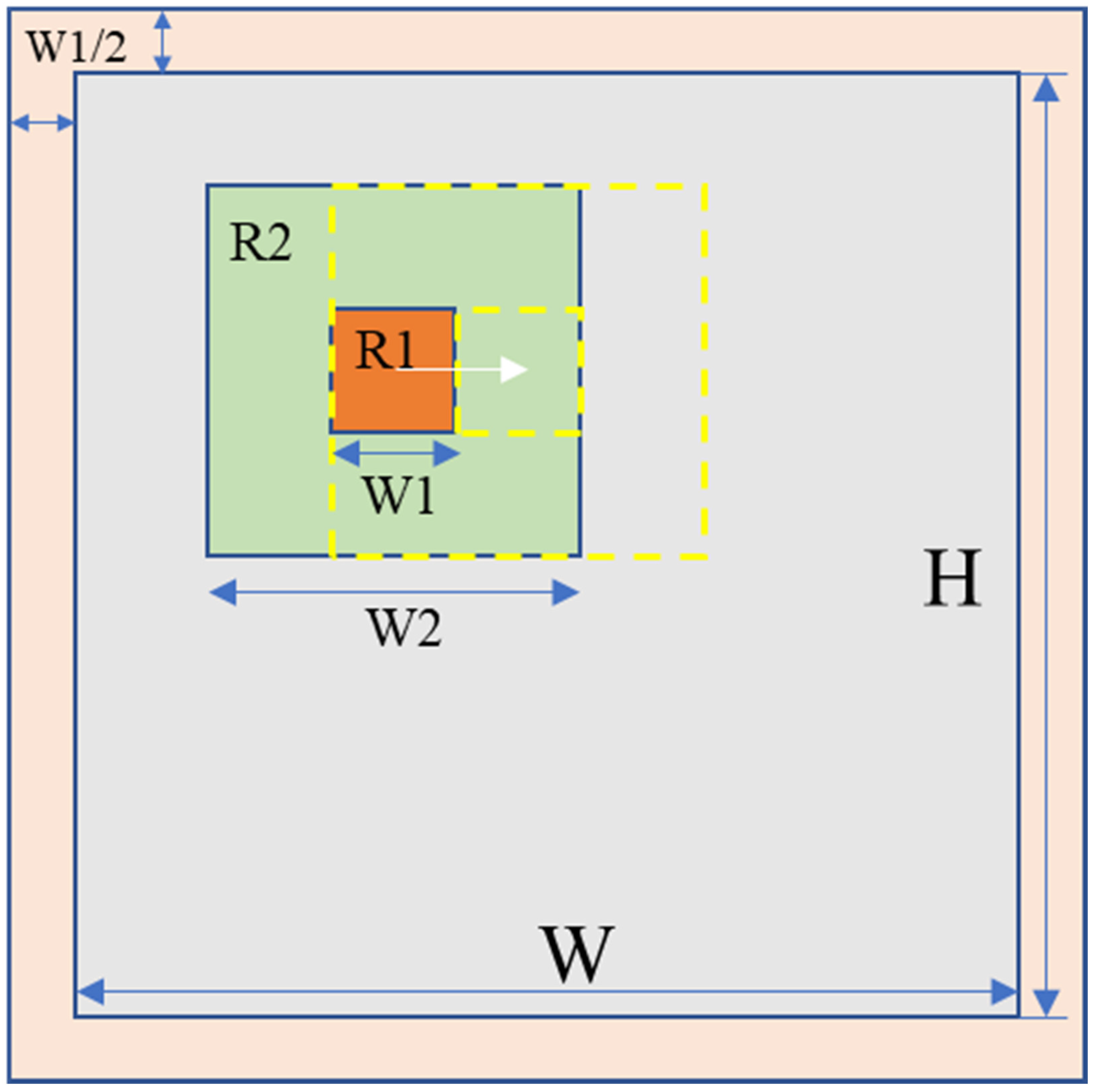
For extracting saliency by the multi-scale filtering method, we set the sizes of the sliding window ( R 1 ) and search window ( R 2 ) as W 1 and W 2 , respectively. Then the absolute value S of the difference between the average of the sliding window and the search window was calculated. S is assigned to all points in the sliding window R 1 . Moving the two windows in the whole image, we obtained the saliency, S i of the image (1 ≤ i N , N is the length of W 1 sequence). Changing the size of R 1 , we got the average saliency of the image by S ¯ = 1 N i = 1 N S i . See Figure 2 and the following for details.
(1)
Set size W 1 for R 1 and W 2 for R 2 (search window). W 1 is a sequence and 1 W 1 i W 2 2 (1 ≤ i N , N is the length of W 1 sequence). For example, W 1 = [ 4   6   8   12   16   24   32 ] ,   W 2 = 140 ;
(2)
Expand the normalized deformation graph by W 1 i 2 and fill it with null values;
(3)
Calculate the average d R 1 ¯ and d R 2 ¯ of the non-null points of R 1 and R 2 ;
(4)
Calculate the saliency S = | d R 1 ¯ d R 2 ¯ | ;
(5)
The saliency of all points in window R 1 is assigned as S ;
(6)
Move R 1 and R 2 until the entire deformation graph is traversed to obtain S i ;
(7)
Repeat steps 2–6 with different W 1 values;
(8)
Calculate the average of multiple saliency graphs S ¯ = 1 N i = 1 N S i .
The saliency extraction of multi-scale filtering is to obtain the average difference between the sliding window (multiple window size) and the search window. This difference is positively correlated to saliency. The sliding windows with different sizes reflect the saliency at different scales, and the average saliency of each scale can reflect the saliency of deformation from local to global.
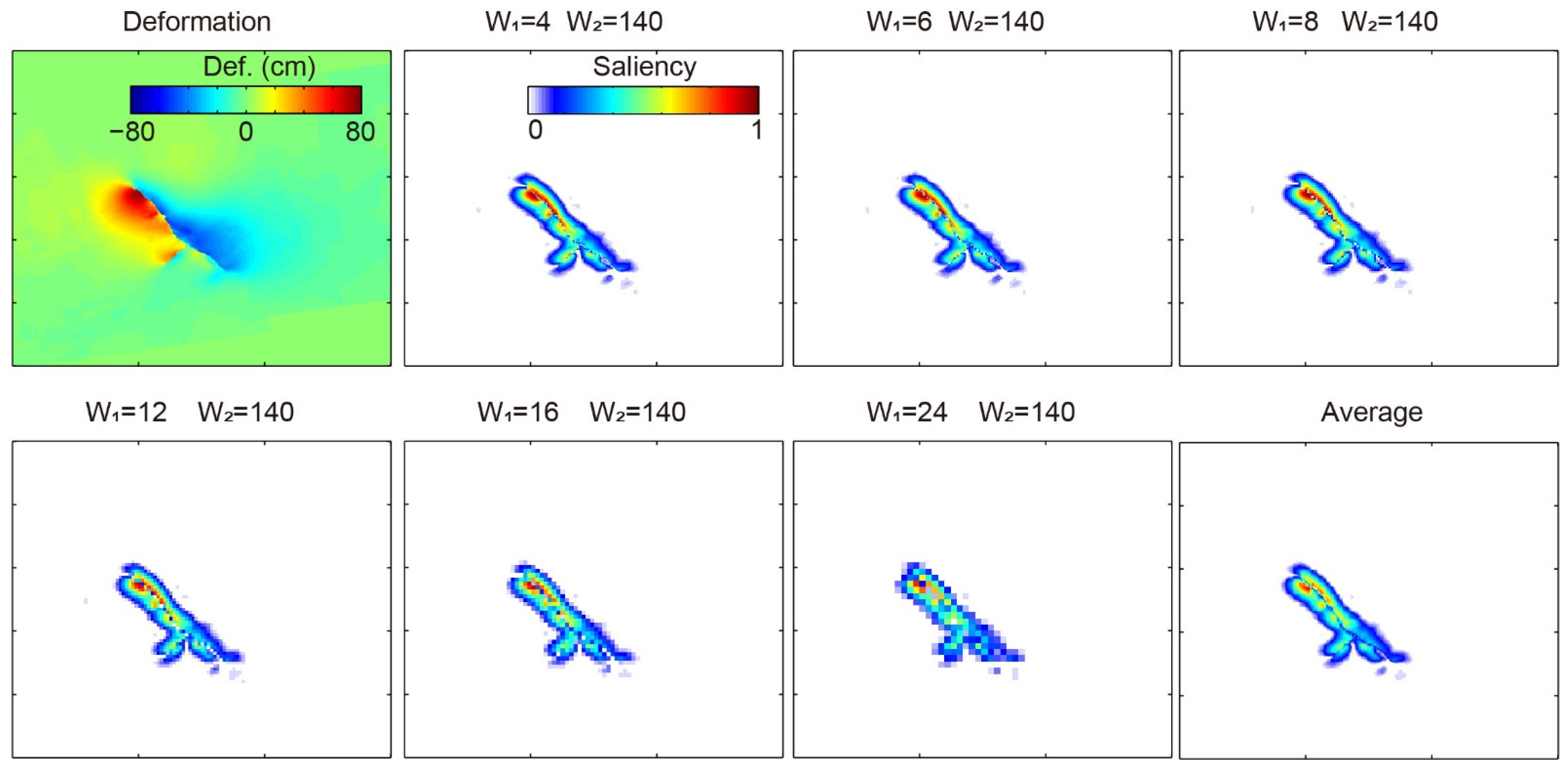
The first panel of Figure 3 is the line-of-sight (LOS) co-seismic deformation of the 2019 Ridgecrest Mw7.1 earthquake obtained by the ascending orbit of Sentinel-1. Other panels of Figure 3 show the saliency graphs of the co-seismic deformation obtained by different W 1 values and the average. With the increase of W 1 , the resolution of the saliency graph decreases gradually, and the saliency of the region R 1 on a larger scale is shown. The size of R 2 is positively correlated to the regional integrity of saliency.
(2) Creating a mask file based on saliency: SQS combines the characteristics of the saliency graph and quadtree algorithm and uses the expansion algorithm for auxiliary processing [16,17,18] (refer to Supplementary Materials Texts S1 and S2 for details). The expansion algorithm can extend the boundary to cover the whole main deformation region. It can also fill the data gap and solve the problems, such as the two sides of the fault partition area so that the major deformation areas into a whole. The mask file processed by the expansion algorithm can distinguish the near-field, far-field, and local deformation. Then, the largest deformation region is selected as the near-field region.
(3) Quadtree sampling based on saliency: The average saliency graph after masking the largest area can preserve the details of the main deformation in the quadtree meshing, so the far-field can be uniformly sampled with the maximum window size. QS takes the standard deviation of the deformation in the window as the reference index. However, SQS uses the standard deviation of saliency ( σ w ) in the window as a reference index. When σ w is greater than the set threshold, the window is equally divided into four windows. Perform iteration until σ w in the partitioned window is smaller than the threshold or the window size is smaller than the minimum size. According to the principle of the quadtree algorithm, the image needs to be cropped or expanded into a matrix with both the length and width of 2n pixels (n = 0, 1, 2…) before sampling.

3. Simulation Experiments

3.1. Simulation Experiment 1: Comparison the Sampling Results between SQS and QS

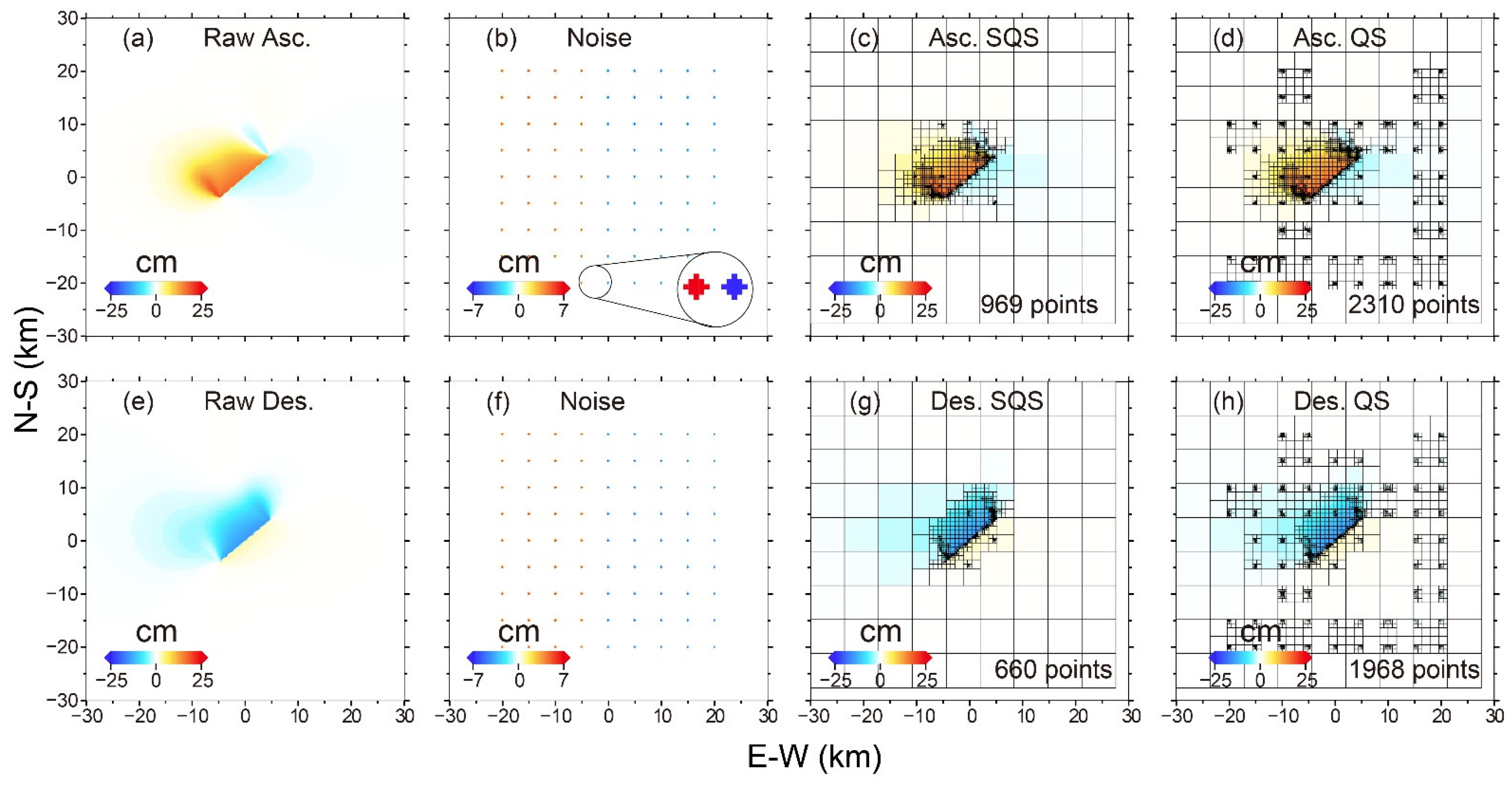
We simulated the deformation of an earthquake, using the Okada model [19]. The Okada model program comes from the code package provided by Stanford University (https://cdfm.stanford.edu/software, last accessed 4 April 2021). The source parameters of the simulated earthquake are shown in SE 1 (Simulation Experiment 1) of Table 1. We simulated the ascending and descending LOS deformation, using the parameters of the Sentinel-1 satellite (Figure 4a,e). The width of the deformation field is 60 km × 60 km. The grid density is set as 600 × 600 pixels, and the resolution of each pixel is set as 100 m. The simulated maximum deformation is 21.8 cm. To test the performance of SQS, regular noise is added to the original deformation field, in which 7.3 cm noise deformation (30% of the maximum deformation) is added to the west side of the deformation field, and −7.3 cm noise is added to the east side (Figure 4b,f).
We used both SQS and QS to sample the simulated deformation fields. For SQS, the deformation is normalized to 0~1, and saliency is calculated with W 1 of [4 6 8 12 16 24] and W 2 of 140. The threshold is 0.08 and 0.1 for ascending and descending images, respectively, when the saliency is binarized. After one expansion, the mask file is generated (Supplementary Materials Figures S1 and S2). Based on the saliency figure and the mask file, we use the minimum and maximum divided windows of 2 and 64, and the threshold σ w of 0.03 to divide the grid. The results of SQS are shown in Figure 4c,g. QS adopts the same maximum and minimum divided windows and uses the threshold of grid partition as 0.5 cm (Table 2). The QS results are shown in Figure 4d,h. SQS effectively reduces the noise in the far-field deformation and retains the details of the near-field deformation. To test whether SQS can distinguish the near-field from the far-field under the condition that the noise level is equal to the deformation level, we tried to increase the magnitude of the noise (±29 cm) to make it larger than the maximum of the main deformation (see Supplementary Materials Figure S3). The results show that SQS can still distinguish the near-field from the far-field and reduce the interference of local deformations.

3.2. Simulation Experiment 2: Linear Inversion Results Based on SQS and QS

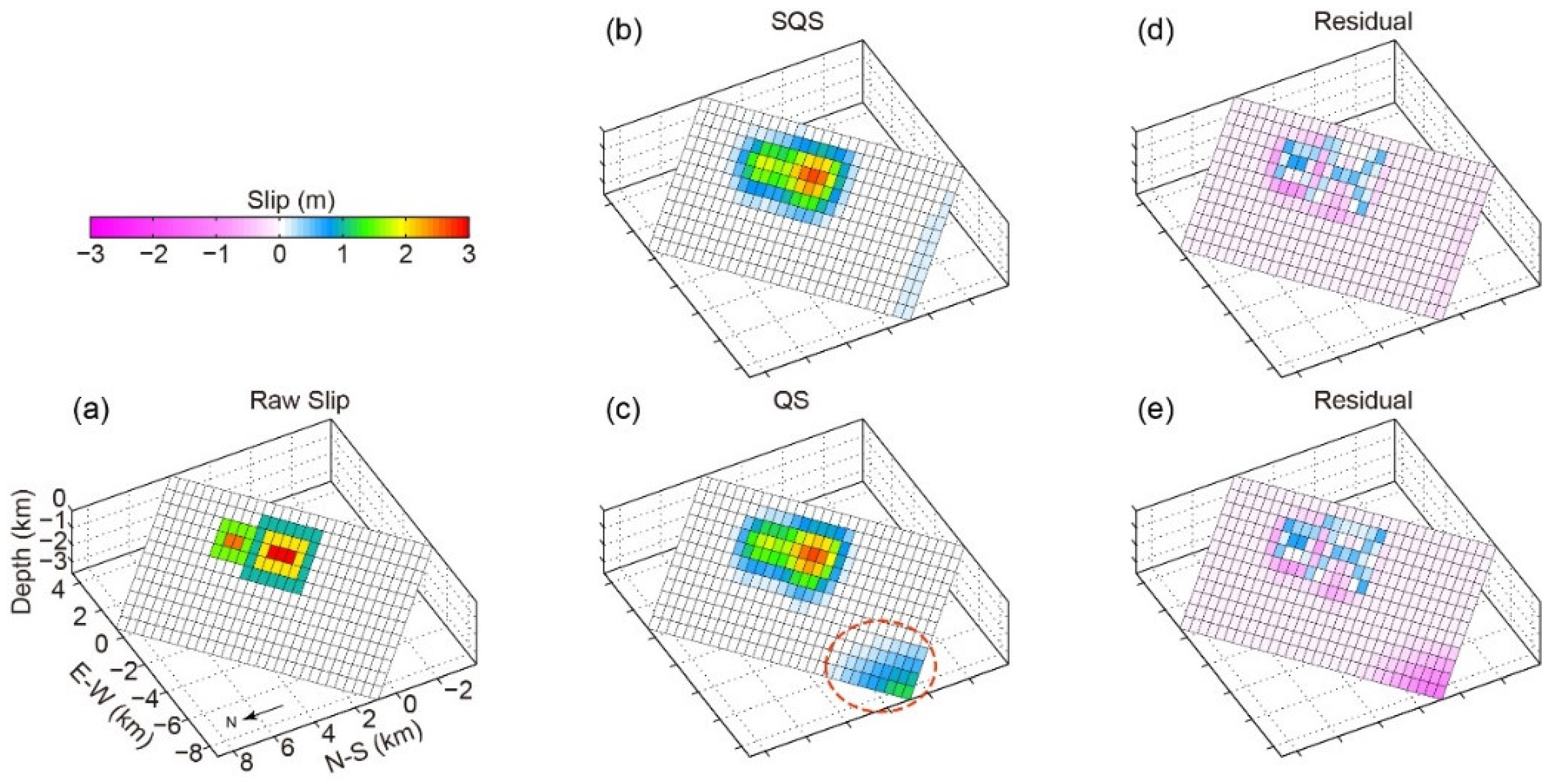
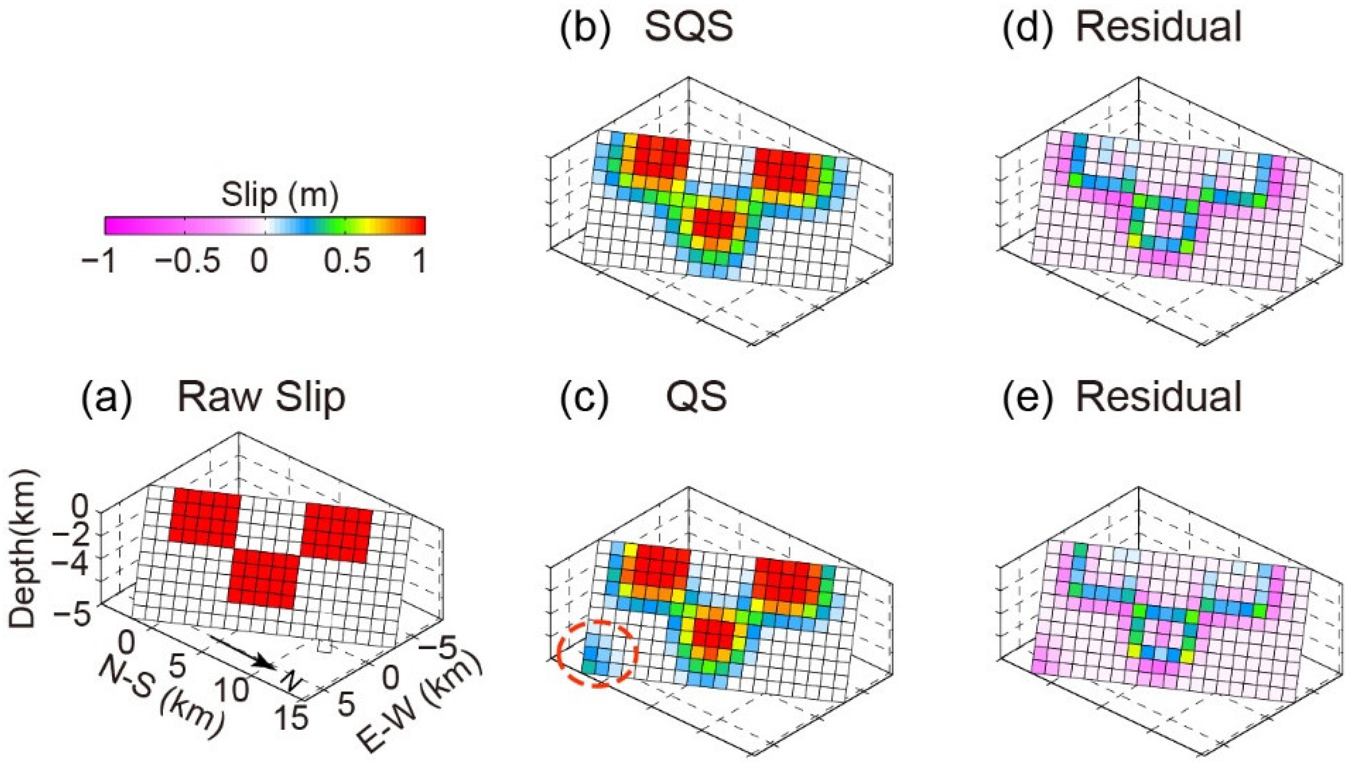
To study the effect of sampling points on inversion results, in simulation experiment 2 (SE 2), we simulated a fault slip as shown in Figure 5a. The geometric parameters of the fault are shown in SE 2 of Table 1. Similar to Section 3.1, we simulated the ascending and descending LOS deformation, using the Sentinel-1 parameters and Okada model, and determined the maximum deformation to be 84.8 cm (descending). We added the atmospheric noise from the real data, with a maximum of 15.2 cm (Figure 6). Then, SQS and QS were used to sample the ascending and descending deformations, and the results are shown in Figure 6. The sampling parameters are shown in Table 2. We used these two sets of sampling results to invert the linear slip distribution separately. Completely consistent non-negative constraints and smoothing factors were adopted in the inversion [10,20] and the inversion results are shown in Figure 5.
As shown in Figure 6, QS fails to distinguish local deformation effectively. Obvious local deformations are observed in the west, southwest, and southeast of the main deformation regions, and unnecessary points were sampled in these regions. SQS effectively differentiated the deformation regions of near-field and far-field. SQS uniformly samples the far-field region with the maximum window and does well when reducing the interference of local deformation. The near-field region is divided by the quadtree algorithm according to the saliency after masking. The inversion results show that the result based on SQS restored the real slip well. Contrarily, there is an obvious inversion error in the results based on QS (Figure 5c), as QS fails to suppresses the local deformation in the far-field.

3.3. Simulation Experiment 3: The Resolution of the Inversion Results Based on SQS and QS

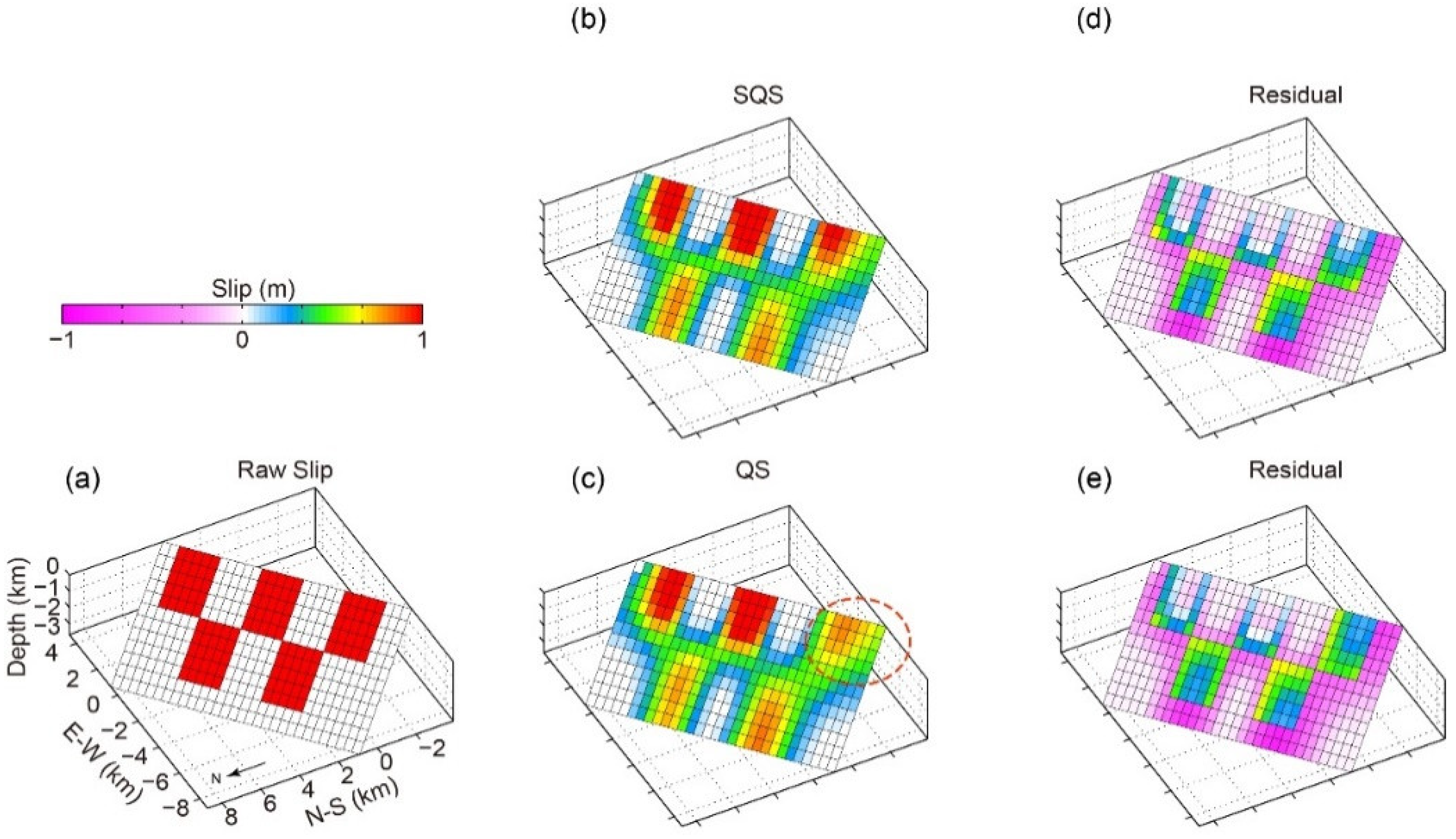
We conducted a checkboard experiment to explore the effect of the two methods on the inversion results, which is simulation experiment 3 (SE 3). We constructed the checkboard slip model as shown in Figure 7a. The fault geometry is shown in SE 3 of Table 1. Based on the location of the sampling points obtained by SQS and QS in Section 3.2, the LOS deformations were forwarded by the checkboard slip model. The maximum random error of ±3 cm was added to the deformation fields. Then, the slip distribution was inverted from these two groups of deformation. The results are shown in Figure 7.
The resolution based on QS is lower in the upper right corner (the red ellipses region in Figure 7) than that based on SQS. The reason is that the local deformation may change the distribution of the sampled points, which disperses the weight of the algorithm to invert the fault slip, and finally, it is reflected in the inversion resolution. Compared with QS, SQS can avoid far-field deformation and obtain better points distribution, to get more reliable inversion results.

4. Case Study

The simulation experiments verify the feasibility and advantages of SQS. This section takes the Dingri earthquake, which occurred on 20 March 2020, as an example to validate the algorithm in dealing with deformation of real earthquake.

4.1. Background

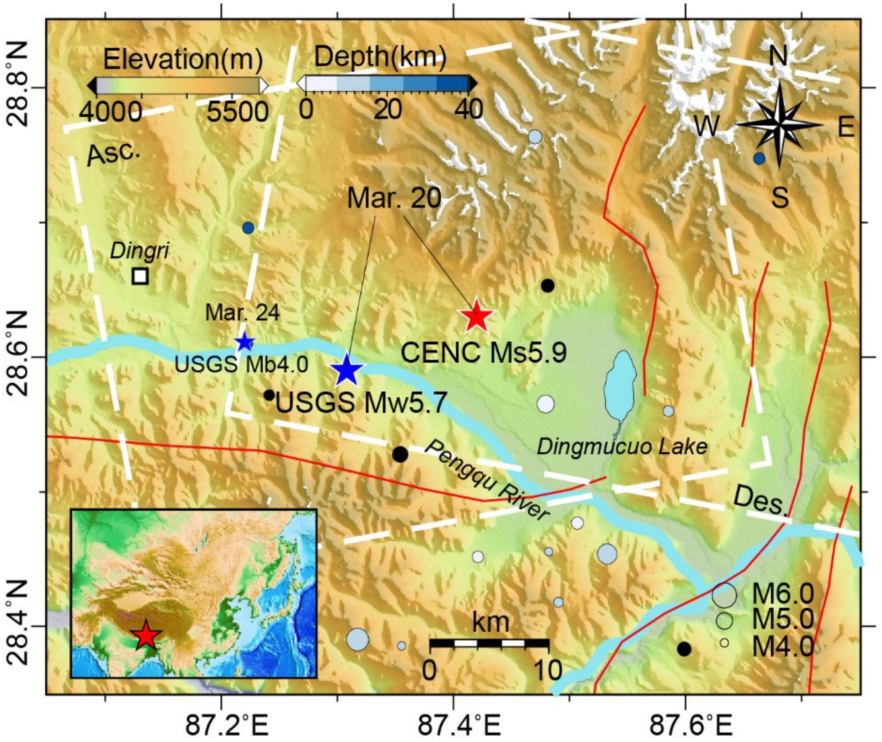
The Rikaze region of China is located on the border between China and Nepal in the northern foothills of the Himalayas. The Rikaze region between the normal fault system of North Himalayan and the Yarlung-Zangbo River fault system [21]. Due to the East–West tension, the normal rift faults of Shenzha-Dingjie and the Dangreyongcuo-Dingri fault are formed in this area [22,23]. Since 1950, 15 M > 5 earthquakes have occurred in the vicinity of Dingri County, Rikaze, the largest of which was M6.2 on 20 March 1993 (United States Geological Survey, USGS, https://www.usgs.gov/natural-hazards/earthquake-hazards/earthquakes, last accessed 4 April 2021). On 20 March 2020, an Ms5.9 earthquake occurred in Dingri, Rikaze (China Earthquake Networks Center, CENC, https://www.cenc.ac.cn/, last accessed 4 April 2021), which was called the Dingri event (Figure 8). As the earthquake area was sparsely populated, the event caused no human or serious property damage. However, since the earthquake occurred on the plate boundary and to the north of the 2015 Nepal Mw 7.8 earthquake [24,25], the Dingri earthquake provides valuable information on plate movement and tectonic characteristics.

4.2. Sampling Results of Co-Seismic Deformations of the Dingri Event

Using the Sentinel-1 data, we obtained the ascending (Path 121, 2020/03/16-2020/03/28) and descending orbits (Path 12, 2020/03/08-2020/03/20) co-seismic deformation fields of the Dingri event (Figure 9 and Figure 10d,g). The deformation caused by the earthquake is concentrated in the northeast of the epicenter (moving away from the satellite) with a small amount of scattering in the southwest. The maximum ascending and descending deformations are 13.8 cm and 14.9 cm, respectively, which are both away from the satellite. The deformation characteristics suggest that the earthquake was caused by a normal fault slip. We use SQS and QS to sample the deformation fields of the earthquake (Figure 9). The sampling parameters are shown in Table 2. The saliency and mask extraction are shown in Supplementary Materials Figures S2 and S4. Due to the river in the south and the lake in the southeast of the seismic area, and some aftershocks, local deformation, and atmospheric interference, the QS method oversamples in these areas. SQS can distinguish the far-field and near-field regions well. The maximum window uniform is used for local deformation regions or far-field deformation areas.

4.3. Source Parameters of the Dingri Event

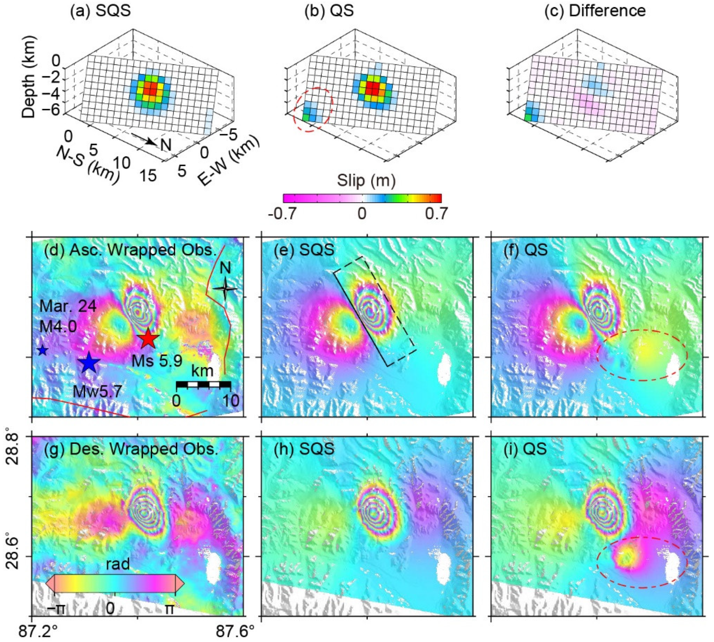
The source parameter results of the nonlinear inversion based on QS and SQS are shown in Table 3. The geometric parameters of the two results are similar, but the motion parameters of QS are larger than those of SQS, since the model based on QS needs a bigger slip to fit the far-field deformation. We used the sampling points obtained by SQS to determine the basic geometric parameters of the fault (Table 3). We extended the fault plane to 20 × 10 km and divided it into 200 slip units with the size of 1 × 1 km. Then the two sampling results were used for linear inversion, using the same non-negative constraints and smoothing factors. As Figure 10 shows, there is an obvious inversion error in the result based on QS (the ellipse region in Figure 10b), as QS fails to suppresses the local deformation in the far-field. The linear inversion results based on SQS indicate that the earthquake is caused by an almost pure normal slip, and the seismic moment is 3.14 × 10¹⁷ Nm, corresponding to Mw 5.63. The main slip of the earthquake is 2.0–5.5 km deep with a maximum of 0.68 m.
A checkboard experiment was carried out for the Dingri earthquake to test the inversion resolution. The checkboard slip model (Figure 11a) is based on the fault geometry inverted by SQS in Table 3. The maximum random error of ±3 cm was added to the forward deformation points. Then, the slip distributions were inverted from these two groups of deformations sampled by QS and SQS. The results are shown in Figure 11.
Using these two slip models we forwarded and wrapped the surface deformation by 2.8 cm per fringe (Figure 10). The red ellipse region in Figure 10f,i is caused by the unreliable asperity in Figure 10b. The checkboard test also shows an abnormal asperity in the inversion result based on QS (Figure 11c), indicating that the inversion results of QS are influenced by the local deformation in the south of the fault. In Figure 10, the forwarded deformation based on SQS points is more consistent with the original deformation field, and the local signals around the lake are ignored. The forwarded descending deformations in the center and the west part of the epicenter (Figure 10h) are slightly lower than the observations, because an M4.0 aftershock occurred 4 days after the mainshock. The ascending secondary image was imaged about just 11 h after the mainshock, so it does not include the aftershock, but the descending secondary image acquired on April 1 includes the deformation of this aftershock. Thus, the overall descending observation is slightly larger than the forwarded result. We obtained the deformation of the M4.0 aftershock using the Sentinel-1 ascending image (Supplementary Materials Figure S5) and confirmed the above analysis. Furthermore we found that the main deformation location of the aftershock is on the northeast of the epicenter provided by USGS (the small blue star in Figure 8), close to the mainshock (the red star in Figure 8), which reflects the advantages of InSAR in earthquake observation and epicenter determination.

5. Discussion

Inverting source parameters of an earthquake from InSAR images requires reliable co-seismic deformation observation. However, due to the atmospheric disturbance, terrain residual, aftershock deformation, local landslide deformation, and noise, deformation observation always contain some errors. On the one hand, the sampling algorithm can keep the original data information as much as possible while reducing the amount of data. On the other hand, it can reduce some noise. In simulation experiment 1, with intensive and big local deformation, SQS weakened and separated the local deformation, and it extracted the far-field and near-field regions. This demonstrates the ability of SQS in restraining local deformation. Simulation experiments 2 and 3 confirm the advantages of SQS and show the effect of sampling points on the inversion results. Good sampling results are conducive to obtain reliable inversion results. The Dingri earthquake is an example to validate the algorithm in dealing with the real deformation of earthquakes. In addition to the Dingri earthquake, we also tested several real earthquake cases with different magnitudes and types based on SQS and QS (2020/2/3 Chengdu Mw4.8 earthquake, 2009/4/6 L’Aquila Mw6.3 earthquake, and 2018/9/28 Palu Mw7.5 earthquake) (Supplementary Materials Figures S6–S8) [10,27]. The sampling parameters are shown in Supplementary Materials Table S1. These cases fully show the feasibility and advantages of SQS in practical application.
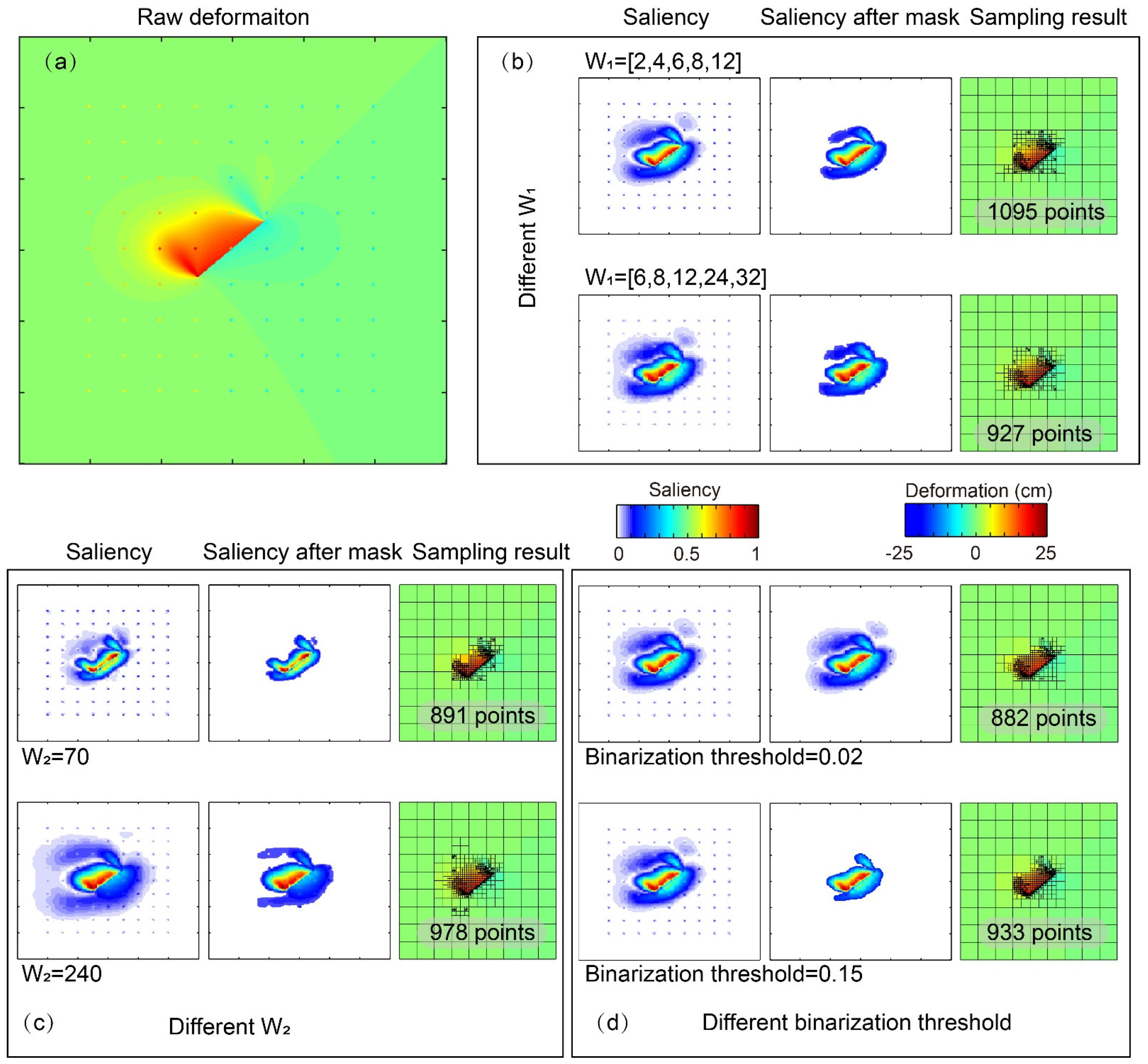
The parameters setting is also an important factor affecting the results of SQS. Moreover, σ w and the maximum and minimum segmentation windows are set according to the demand. If more points and more detailed information are needed to be displayed, the σ w and maximum and minimum segmentation windows can be reduced, and vice versa. W 1 , W 2 , and the binarization threshold affect the segmentation of near-field and far-field. The smaller the W 1 or the longer the sequence is, the more detailed the saliency is. W 2 can affect the overall shape of the saliency figure. Generally, the larger the W 2 is, the larger the near-field range is. Figure 12 shows how the results change when these parameters change independently. The raw deformation in Figure 12 is same as Figure 4a. SQS parameters used in Figure 12b–d are consistent with SE 1 Ascending in Table 2, except for the parameters indicating the changes. For the results in Figure 12, SQS can separate near-field deformation and far-field deformation no matter how the parameters change, but different parameter settings will affect the size of the near-field region and sampling details. With the increase of W 1 , the resolution of the saliency graph decreases gradually. However, it has only a small effect on the size of the near-field region. When W 2 is too small or the binarization threshold is too large, the area of the near-field region is small. However, the small near-field area does not mean the little sampling points. Figure 12d shows that different sizes of near-field are obtained due to different binarization thresholds. Due to the normalization, the results with a small near-field area highlight the saliency differences, so more points can be obtained in the near-field. We tried many experiments, and the changes of sampling points with W 2 and binarization threshold are shown in Supplementary Materials Figure S9. The results show that the number of sampling points is not positively or negatively correlated with W 2 and binarization threshold. In other words, the number of sampling points does not simply increase with the area of the near-field. In a certain range, increasing W 2 or the binarization threshold can increase the number of sampling points. However, when it reaches a peak, the number of sampling points will decrease. We need to select parameters according to our needs, to obtain the appropriate near-field region and sampling points.
The points sampled by SQS can obtain better inversion results of slip distribution than QS. However, the improvement of the sampling algorithm for seismic inversion results is not constant. When the deformation interference of far-field is small and the main deformation is concentrated, the results of QS and SQS are not significantly different, and the inversion results obtained by them are similar. For example, the local deformation far away from the main deformation areas has little contribution to the inversion, which can be ignored by the inversion algorithm. In such cases, the advantage of SQS is not obvious. Besides, if the far-field deformation is very large or complex, SQS can hardly distinguish the near-field from the far-field deformation (QS cannot distinguish it even more). However, in the actual research, these extreme situations are rare. Usually, the co-seismic deformation obtained by InSAR is mainly co-seismic deformation, and it will be affected by local deformation, atmospheric error, or noise, resulting in local high deformation gradient region [10,20,24,27,28,29] (Supplementary Materials Figures S6–S8). In these cases, SQS will have different degrees of improvement compared with QS. Reliable inversion results are based on reliable original deformation data. Therefore, when the deformation field is seriously influenced by noises or errors, we should reduce these noises and errors first, instead of only relying on a sampling algorithm.

6. Conclusions

We proposed an improved quadtree sampling method based on saliency. The method is simple and efficient and can get optimized sampling data for seismic deformation. SQS can retain the deformation details of the main deformation area and restrain the impact of the far-field or local deformation, to facilitate the subsequent inversion and other researches. Furthermore, unlike the resolution-based sampling algorithm, SQS does not need prior fault parameters. The simulation experiments and real cases show the advantages of the proposed algorithm in reducing the amount of data and the interference of far-field or local deformation to the inversion results. However, due to the simplicity of the extraction saliency method we adopted, the expansion algorithm and area calculation are still needed after extraction saliency. Further researches could be focused on improving the SQS by omitting subsequent treatment and reducing parameters that need to be set manually. This research obtained the co-seismic deformation field, fault geometric parameters, and slip distribution of the Dingri earthquake, which provides references for studies on this earthquake.

Supplementary Materials

The following are available online at https://www.mdpi.com/article/10.3390/rs13091678/s1. Text 1: the details of the expansion process. Text 2: Details of region area calculation and region selection. Figure S1: Deformation, saliency under different filtering windows, and saliency average of simulation experiments. Figure S2: Binary graph, expanded result, mask, and masked saliency of simulation experiments and the Dingri event. Figure S3: Results of SQS and QS with noise amplitude same as the deformation. Figure S4: Deformation, saliency under different filtering windows, and their average of the Dingri event. Figure S5: Deformation of the M4.0 aftershock observed by Sentinel-1. Figure S6: SQS and QS results of the 2020 Mw4.8 Chengdu earthquake. Figure S7: SQS and QS results of the 2009 Mw6.3 L’Aquila earthquake. Figure S8: SQS and QS results of the 2018 Mw7.5 Palu earthquake. Figure S9: Sampling numbers of SQS with different parameters. Table S1: Parameters used in sampling deformation fields of Supplementary Figures S6, S7, and S8.

Author Contributions

H.G. performed the data processing, improved algorithm, source parameter inversion, and drafted the manuscript. M.L. and G.F. provided helpful suggestions and revised the manuscript. All authors have read and agreed to the published version of the manuscript.

Funding

This work is supported by the National Key Research and Development Program of China (Grant No. 2019YFC1509201), the National Natural Science Foundation of China (Grant No. 41904001), the China Postdoctoral Science Foundation (Grant No. 2018M640733), and the National Postdoctoral Program for Innovative Talents (Grant No. BX20180220).

Data Availability Statement

The deformation data of the Dingri earthquake and Matlab code of SQS are available in Supplementary Materials.

Acknowledgments

We thank five anonymous reviewers for their thoughtful comments. The Sentinel-1 and Envisat images are from Copernicus Open Access Hub (https://scihub.copernicus.eu/, last accessed 4 April 2021) of the European Space Agency (ESA). The ALOS-2 images are from JAXA under Project P1390002. Part of the figures in this paper were prepared with the Generic Mapping Tools.

Conflicts of Interest

The authors declare no conflict of interest.

References

  1. Massonnet, D.; Rossi, M.; Carmona, C.; Adragna, F.; Peltzer, G.; Feigl, K.; Rabaute, T. The displacement field of the Landers earthquake mapped by radar interferometry. Nature 1993, 364, 138–142. [Google Scholar] [CrossRef]
  2. Biggs, J.; Wright, T.J. How satellite InSAR has grown from opportunistic science to routine monitoring over the last decade. Nat. Commun. 2020, 11, 1–4. [Google Scholar] [CrossRef]
  3. Simons, M. Coseismic Deformation from the 1999 Mw 7.1 Hector Mine, California, Earthquake as Inferred from InSAR and GPS Observations. Bull. Seism. Soc. Am. 2002, 92, 1390–1402. [Google Scholar] [CrossRef]
  4. He, P.; Wen, Y.; Ding, K.; Xu, C. Normal Faulting in the 2020 Mw 6.2 Yutian Event: Implications for Ongoing E–W Thinning in Northern Tibet. Remote Sens. 2020, 12, 3012. [Google Scholar] [CrossRef]
  5. Ross, Z.E.; Idini, B.; Jia, Z.; Stephenson, O.L.; Zhong, M.; Wang, X.; Zhan, Z.; Simons, M.; Fielding, E.J.; Yun, S.-H.; et al. Hierarchical interlocked orthogonal faulting in the 2019 Ridgecrest earthquake sequence. Science 2019, 366, 346–351. [Google Scholar] [CrossRef] [Green Version]
  6. Pritchard, M.E.; Simons, M.; Rosen, P.A.; Hensley, S.; Webb, F.H. Co-seismic slip from the 1995 July 30Mw = 8.1 Antofagasta, Chile, earthquake as constrained by InSAR and GPS observations. Geophys. J. Int. 2002, 150, 362–376. [Google Scholar] [CrossRef] [Green Version]
  7. Jonsson, S. Fault Slip Distribution of the 1999 Mw 7.1 Hector Mine, California, Earthquake, Estimated from Satellite Radar and GPS Measurements. Bull. Seism. Soc. Am. 2002, 92, 1377–1389. [Google Scholar] [CrossRef]
  8. Lohman, R.B.; Simons, M. Some thoughts on the use of InSAR data to constrain models of surface deformation: Noise structure and data downsampling. Geochem. Geophys. Geosyst. 2005, 6. [Google Scholar] [CrossRef]
  9. Wang, C.; Ding, X.; Li, Q.; Jiang, M. Equation-Based InSAR Data Quadtree Downsampling for Earthquake Slip Distribution Inversion. IEEE Geosci. Remote. Sens. Lett. 2014, 11, 2060–2064. [Google Scholar] [CrossRef]
  10. Wang, L.; Gao, H.; Feng, G.; Xu, W. Source parameters and triggering links of the earthquake sequence in central Italy from 2009 to 2016 analyzed with GPS and InSAR data. Tectonophysics 2018, 744, 285–295. [Google Scholar] [CrossRef]
  11. Gao, H. Research on InSAR Seismic Source Parameter Inversion and the Triggering Relationship between Earthquake. Master’s Thesis, East China University of Technology, Nanchang, China, 2018. (In Chinese with English Abstract). [Google Scholar]
  12. Itti, L.; Koch, C.; Niebur, E. A model of saliency-based visual attention for rapid scene analysis. IEEE Trans. Pattern Anal. Mach. Intell. 1998, 20, 1254–1259. [Google Scholar] [CrossRef] [Green Version]
  13. Zhai, Y.; Shah, M. Visual attention detection in video sequences using spatiotemporal cues. In Proceedings of the 14th Annual ACM International Conference on Multimedia—MULTIMEDIA’06, Barbara, CA, USA, 21–25 October 2006; pp. 815–824. [Google Scholar] [CrossRef]
  14. Goferman, S.; Zelnik-Manor, L.; Tal, A. Context-Aware Saliency Detection. IEEE Trans. Pattern Anal. Mach. Intell. 2011, 34, 1915–1926. [Google Scholar] [CrossRef] [PubMed] [Green Version]
  15. Achanta, R.; Estrada, F.; Wils, P.; Süsstrunk, S. Salient Region Detection and Segmentation. In Proceedings of the Lecture Notes in Computer Science, Sydney, NSW, Australia, 14–18 September 2008; pp. 66–75. [Google Scholar]
  16. Boomgaard, R.V.D.; Van Balen, R. Methods for fast morphological image transforms using bitmapped binary images. CVGIP Graph. Model. Image Process. 1992, 54, 252–258. [Google Scholar] [CrossRef]
  17. Haralick, R.M.; Linda, G.S. Computer and Robot Vision; Addison-Wesley: Boston, MA, USA, 1992; Volume I, pp. 28–48. [Google Scholar]
  18. Gonzalez, R.C.; Woods, R.E.; Eddins, S.L. Digital Image Processing Using MATLAB; Pearson Education India: Chennai, India, 2004. [Google Scholar]
  19. Okada, Y. Surface deformation due to shear and tensile faults in a half-space. Bull. Seismol. Soc. Am. 1985, 75, 1135–1154. [Google Scholar]
  20. Wang, L.Y.; Gao, H.; Feng, G.C. Triggering relations and stress effects analysis of two Mw> 6 earthquakes in southwest Taiwan based on InSAR and GPS data. Acta Geod. Cartogr. Sin. 2019, 48, 1244. [Google Scholar] [CrossRef]
  21. Yin, A.; Harrison, T.M. Geologic Evolution of the Himalayan-Tibetan Orogen. Annu. Rev. Earth Planet. Sci. 2000, 28, 211–280. [Google Scholar] [CrossRef] [Green Version]
  22. Li, P.; Qing, S.Q.; Chen, K. On the seismogenic process of the 25 April 2015 Mw7.8 earthquake and future earthquake situation. China J. Geophys. 2015, 58, 1827–1833, (In Chinese with English Abstract). [Google Scholar]
  23. Wang, Y.Z.; Chen, S.; Chen, K. Source Model and Tectonic Implications of the 2020 Dingri Mw5.7 Earthquake Constrained by InSAR Data. Earthquake 2021, 41, 116–128, (In Chinese with English Abstract). [Google Scholar]
  24. Feng, G.; Li, Z.; Shan, X.; Zhang, L.; Zhang, G.; Zhu, J. Geodetic model of the 2015 April 25 Mw 7.8 Gorkha Nepal Earthquake and Mw 7.3 aftershock estimated from InSAR and GPS data. Geophys. J. Int. 2015, 203, 896–900. [Google Scholar] [CrossRef] [Green Version]
  25. Egoda, K.; Ekiyota, T.; Epokhrel, R.M.; Echiaro, G.; Ekatagiri, T.; Esharma, K.; Ewilkinson, S. The 2015 Gorkha Nepal Earthquake: Insights from Earthquake Damage Survey. Front. Built Environ. 2015, 1, 8. [Google Scholar] [CrossRef]
  26. Deng, Q.D.; Zhang, P.Z.; Ran, Y.K.; Yang, X.P.; Min, W.; Chu, Q.Z. Basic characteristics of active tectonics in China. Sci. China Ser. D Earth Sci. 2002, 32, 1020–1030, (In Chinese with English Abstract). [Google Scholar]
  27. He, L.; Feng, G.; Li, Z.; Feng, Z.; Gao, H.; Wu, X. Source parameters and slip distribution of the 2018 M 7.5 Palu, Indonesia earthquake estimated from space-based geodesy. Tectonophysics 2019, 772, 228216. [Google Scholar] [CrossRef]
  28. Sudhaus, H.; Jónsson, S. Improved source modelling through combined use of InSAR and GPS under consideration of correlated data errors: Application to the June 2000 Kleifarvatn earthquake, Iceland. Geophys. J. Int. 2009, 176, 389–404. [Google Scholar] [CrossRef] [Green Version]
  29. Ding, K.; He, P.; Wen, Y.; Chen, Y.; Wang, D.; Li, S.; Wang, Q. The 2017 Mw 7.3 Ezgeleh, Iran earthquake determined from InSAR measurements and teleseismic waveforms. Geophys. J. Int. 2018, 215, 1728–1738. [Google Scholar] [CrossRef]
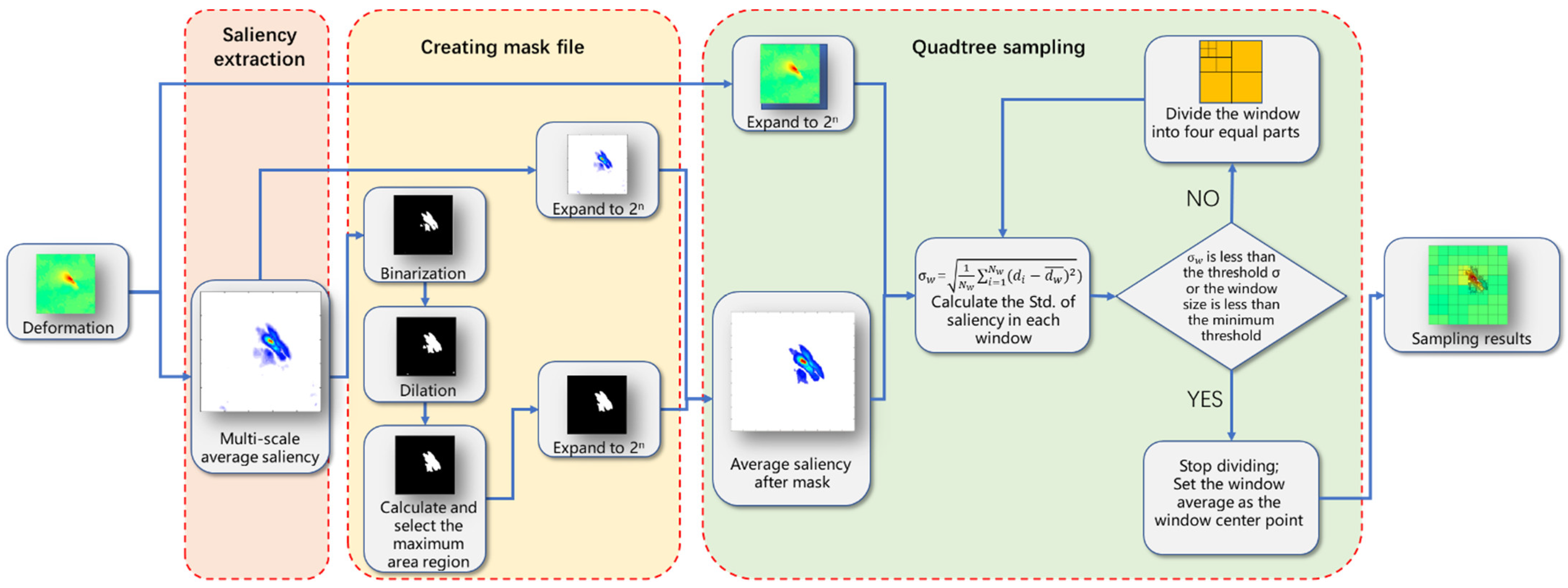
Figure 1. The flowchart of the SQS algorithm.
Remotesensing 13 01678 g001
Figure 2. Multi-scale filter saliency extraction. The gray area is the original map. The pink expansion area fills in the null value. When extracting the average saliency of an image, W 2 is fixed and W 1 is a sequence. The result is the average of the saliency results with different W 1 .
Remotesensing 13 01678 g002
Figure 3. Saliency graphs of co-seismic deformation of the 2019 Mw7.1 Ridgecrest earthquake obtained by different filter window sizes and their average. The co-seismic deformation was obtained from the ascending orbit of Sentinel-1.
Remotesensing 13 01678 g003
Figure 4. SQS and QS results of simulation experiment 1. (a,e) Raw LOS deformation based on the parameters of SE 1 in Table 1. (b,f) Deformation fields with regular noise (±7.3 cm). (c,g) SQS results and (d,h) QS results of the ascending and descending deformation. The warm color denotes the deformation toward the satellite, and the cool color denotes that away from the satellite. The sampling parameters are shown in Table 2.
Remotesensing 13 01678 g004
Figure 5. The linear inversion results obtained using the SQS and QS sampling points. (a) Input slips. (b,c) Inverted slip based on SQS and QS. (d,e) Residuals between the inverted and input slips. The geometry of fault is based on the parameters of SE 2 in Table 1.
Remotesensing 13 01678 g005
Figure 6. SQS and QS results of simulation experiment 2. The raw LOS deformation is based on the parameters of SE 2 in Table 1 and Figure 5. The noise is based on the atmospheric noise from the real data, with a maximum of 15.2 cm. The sampling parameters are shown in Table 2.
Remotesensing 13 01678 g006
Figure 7. Resolution of the inversion results based on the point sampled by SQS and QS. (a) Input slips. (b,c) Inverted slips based on SQS and QS. (d,e) Residuals between the inverted models and input slips. The fault geometry is based on the parameters shown in SE 3 of Table 1.
Remotesensing 13 01678 g007
Figure 8. Geological background and data coverage of the study area. Big stars are the epicenter of the Dingri earthquake provided by CENC and USGS. The small blue star is the epicenter of the M4.0 aftershock provided by USGS. Circles are the historical earthquakes, and the color indicates the depth. Red lines are faults [26]. White dotted lines are the coverages of SAR data.
Remotesensing 13 01678 g008
Figure 9. SQS and QS results of the deformation fields of the Dingri event. (a,c) Ascending and descending results based on SQS. (b,d) Ascending and descending results based on QS.
Remotesensing 13 01678 g009
Figure 10. Slip distribution models based on SQS (a) and QS (b) points and the difference (c); wrapped deformation of Dingri event (d,g); forward results based on figures a (e,h) and b (f,i) respectively.
Remotesensing 13 01678 g010
Figure 11. Inversion resolution of the Dingri event based on the points sampled by SQS and QS. (a) Input slips. (b,c) Inverted slip based on SQS and QS results. (d,e) Residuals between the inverted models and input slips.
Remotesensing 13 01678 g011
Figure 12. Difference of SQS results with different parameters. (a) Raw deformation. (b) Difference in results when only W 1 was changed. (c) Difference in results when only W 2 was changed. (d) Difference in results when only the binarization threshold was changed. The parameters used in the figures are consistent with SE 1 Ascending in Table 2, except for the parameters indicating the changes.
Remotesensing 13 01678 g012
Table 1. Fault parameters used in the simulation experiments.
Length
(km)
Width
(km)
Depth 1
(km)
Strike
(°)
Dip
(°)
Rake
(°)
Strike Slip
(m)
Dip Slip
(m)
Mw
SE 112.237.280305000.4206.00
SE 2 2//03050−900Figure 5a5.79
SE 3 2//03050−900Figure 7a6.26
1 Fault top depth. 2 The size of each patch in SE 2 and SE 3 is 0.4 × 0.6 km, and the slip value should refer to the color bar in Figures 5a and 7a.
Table 2. Parameters used for sampling.
EventMethodWindow SegmentationSaliency
Min windowMax windowSegmentation thresholdBinarization thresholdW1W2Expansion times
SE 1 AscendingSQS2640.030.08[4 6 8 12 16 24]1401
QS2640.5 cm/
SE 1 DescendingSQS2640.030.1[4 6 8 12 16 24]1401
QS2640.5 cm/
SE 2 AscendingSQS2640.030.02[4 6 8 12 16]501
QS2641.7 cm/
SE 2 DescendingSQS2640.030.02[4 6 8 12 16]501
QS2642.7 cm/
Dingri event AscendingSQS81280.030.03[8 12 16 24 32 48 64]2001
QS81280.3 cm/
Dingri event DescendingSQS81280.030.03[8 12 16 24 32 48 64]2001
QS81280.3 cm/
Table 3. Source parameters of nonlinear inversion of the Dingri event based on QS and SQS.
MethodLength
(km)
Width
(km)
Depth 1
(km)
Strike
(°)
Dip
(°)
Rake
(°)
Strike Slip
(m)
Dip Slip
(m)
Mw
QS3.72.72.433055−1130.410.975.63
SQS3.92.92.233052−960.090.815.59
1 Fault top depth.
Publisher’s Note: MDPI stays neutral with regard to jurisdictional claims in published maps and institutional affiliations.