Article

An Improved Method Combining ANN and 1D-Var for the Retrieval of Atmospheric Temperature Profiles from FY-4A/GIIRS Hyperspectral Data

1
Key Laboratory of Infrared System Detection and Imaging Technologies, Shanghai Institute of Technical Physics, Chinese Academy of Sciences, Shanghai 200083, China
2
University of Chinese Academy of Sciences, Beijing 100049, China
3
Shanghai Institute of Technical Physics, Chinese Academy of Sciences, Shanghai 200083, China
4
National Satellite Meteorological Center, Beijing 100081, China
*
Author to whom correspondence should be addressed.
Remote Sens. 2021, 13(3), 481; https://doi.org/10.3390/rs13030481
Submission received: 17 December 2020 / Revised: 21 January 2021 / Accepted: 21 January 2021 / Published: 29 January 2021
(This article belongs to the Special Issue Advances in Infrared Observation of Earth's Atmosphere)

Abstract

:
In our study, a retrieval method of temperature profiles is proposed which combines an improved one-dimensional variational algorithm (1D-Var) and artificial neural network algorithm (ANN), using FY-4A/GIIRS (Geosynchronous Interferometric Infrared Sounder) infrared hyperspectral data. First, according to the characteristics of the FY-4A/GIIRS observation data using the conventional 1D-Var, we introduced channel blacklists and discarded the channels that have a large negative impact on retrieval, then used the information capacity method for channel selection and introduced a neural network to correct the satellite observation data. The improved 1D-Var effectively used the observation information of 1415 channels, reducing the impact of the error of the satellite observation and radiative transfer model, and realizing the improvement of retrieval accuracy. We subsequently used the improved 1D-Var and ANN algorithms to retrieve the temperature profiles, respectively, from the GIIRS data. The results showed that the accuracy when using ANN is better than using improved 1D-Var in situations where the pressure ranges from 800 hPa to 1000 hPa. Therefore, we combined the improved 1D-Var and ANN method to retrieve temperature profiles for different pressure levels, calculating the error by taking sounding data published by the University of Wyoming as the true values. The results show that the average error of the retrieved temperature profiles is smaller than 2 K when using our method, this method makes the accuracy of the retrieved temperature profiles superior to the accuracy of the GIIRS products from 10 hPa to 575 hPa. All in all, through the combination of the physical retrieval method and the machine learning retrieval method, this paper can certainly provide a reference for improving the accuracy of products.

1. Introduction

Infrared satellite hyperspectral vertical detection of atmospheric state can obtain abundant atmospheric spectral information and be able to distinguish more detailed atmospheric vertical structure [1,2,3]. The atmospheric temperature profile is an important atmospheric parameter. Using infrared hyperspectral data, combined with relevant atmospheric infrared radiative transfer models and using 1DVar, neural networks, and other methods to retrieve atmospheric temperature profiles becomes a powerful method for the large-scale, high-frequency, and high-precision acquisition of atmospheric temperature and humidity profiles [4,5].
Fengyun-4A (FY-4A), a new generation of geostationary orbit meteorological satellites for quantitative remote sensing applications in China, was successfully launched on 11 December 2016. Geosynchronous Interferometric Infrared Sounder (GIIRS) is the first instrument in the world to detect the vertical atmospheric structure by means of infrared interferometry spectroscopy in geostationary orbit [6,7,8]. Its primary instrument is a time-modulated Fourier transform spectrometer, whose main purpose is to implement the vertical structure observation of atmospheric temperature and humidity parameters, to improve the resolution of meteorological vertical observation, and to provide services for numerical prediction, weather monitoring, and atmospheric chemical composition detection [9]. Luo et al. [10] evaluated the FY-4A/GIIRS retrieval ability of atmospheric temperature, humidity, ozone, and other atmospheric compositions with Entropy Reduction (ER) and Degrees of Freedom for Signal (DFS) as criteria, combining them with the 1976 American standard atmospheric profile database. The results showed that the ER of temperature and humidity was 37.53 and 28.79, and the DFS for the signal was 10.78 and 8.08, respectively.
At present, the main retrieval methods [11] of temperature and humidity profiles using infrared hyperspectral data include feature vector statistical regression, artificial neural network, and physical methods. Guan et al. [12], Jiang et al. [13], and Zhang et al. [14] used spectral radiance observations from Atmospheric Infrared Sounder (AIRS) to retrieve atmospheric temperature and humidity profiles in China using feature vector statistical regression. The results showed that the obtained temperature and humidity profiles were nearly consistent with the data distribution of the European Centre for Medium-Range Weather Forecasts (ECMWF). Ma et al. [15] used a feature vector method to obtain the initial profile, then used Newton’s nonlinear iterative method to further improve the retrieval accuracy. Although the calculation of the feature vector method is quick and simple, it cannot consider the whole of the physical process of atmospheric radiative transfer, result in a poor retrieval accuracy.
The development of ANN can effectively improve the accuracy and speed of atmospheric remote sensing retrieval [16,17,18,19,20], among which Cabrera Mercader C.R., et al. [21] used the ANN retrieval algorithm to retrieve the atmospheric humidity profiles respectively on land and sea. The results showed that the RMSE of relative humidity was 6–14% over the ocean and 6–15% over the land. Cai [22] also retrieved FY-4A/GIIRS atmospheric temperature and humidity profiles using ANN and used AIRS related products for verification. The results showed that the average temperature RMSE in the troposphere was less than 1 K, and the humidity below 200 hPa was better than 10%. However, the ANN retrieval algorithm is not suitable for areas where data is scarce and there are not enough training samples. Therefore, ANN cannot construct a representative retrieval model for these locations [23,24].
The physical retrieval method takes into account the process of atmospheric radiative transfer and is not dependent on sample training [25,26]. Guan et al. [1] used IASI (Infrared Atmospheric Sounding Interferometer) infrared hyperspectral data and 1D-Var to retrieve atmospheric temperature and humidity profiles. The retrieval results showed that the absolute error for the temperature average value was less than 0.6 K, and the average absolute value of error for the water vapor mixing ratio was less than 0.022 g/kg. Shen et al. [27] used CrIS satellite data and obtained retrieval results of atmospheric temperature and humidity profiles using the NOAA Unique Combined Atmospheric Processing System (NUCAPS) algorithm, indicating that the accuracy was less than 20% when the height of humidity profiles was below 300 hPa. However, the accuracy increases to 30% when the height of humidity profiles was above 300 hPa. Zhu et al. [28] used HIRAS, an infrared hyperspectral atmospheric detector carried by the FY-3D polar orbit meteorological satellite, to retrieve atmospheric temperature and humidity profiles using the 1D-Var retrieval algorithm. The retrieval results are superior to the priori profile as a whole, among which the RMSE of temperature profiles below 100 hPa was less than 1.5 K, the partial pressure level was less than 1 K, and the RMSE of humidity profiles was less than 10% as a whole. Polar orbit satellites are excellent at detecting temperature and humidity information. Geostationary orbit satellites also have the advantages of both high spectral resolution and high temporal resolution to retrieve atmospheric temperature and humidity profiles, as well as being able to detect the rapidly changing mesoscale atmospheric environment and provide higher time resolution temperature and humidity changing information in certain areas.
Based on the FY-4A/GIIRS interferometer atmospheric vertical detector, this study proposes an improved FY-4A/GIIRS retrieval method combining ANN retrieval algorithm with an improved 1D-Var retrieval algorithm. This algorithm mainly includes channel blacklist establishment, temperature channel selection through the information capacity method, observation error correction through the ANN algorithm, Radiative Transfer for TOVS (RTTOV) rapid radiative transfer model, the iterative solution of Optimal Estimation Method (OEM) in the 1D-Var retrieval method, and the integration of the ANN retrieval algorithm which is used to retrieve specific parts of the vertical atmospheric pressure level. In this context, the accuracy of retrieval results was verified using sounding data published by the University of Wyoming, and we compared the accuracy of GIIRS temperature profile products and retrieval temperature profiles of our method. Meanwhile, we analyzed the detection capability of the FY-4A/GIIRS infrared hyperspectral atmospheric vertical detector for atmospheric temperature.

2. Datasets and Model

2.1. Datasets

2.1.1. FY-4A/GIIRS Data

The performance parameters of the FY-4A/GIIRS instrument are shown in Table 1. GIIRS was composed of 32 × 4 pixels surface array detectors to improve the detection sensitivity by long time integration. The interferometer had 1650 channels, which could achieve high resolution continuous spectral coverage of infrared radiation to the earth and atmosphere [29,30,31].
The satellite observation data in our study mainly used the FY-4A/GIIRS interferometer L1 level data after radiometric calibration and geographical positioning (http://satellite.nsmc.org.cn/PortalSite/Data/Satellite.aspx). The data used in our experiment was mainly located in India, and the time is 00:00, 06:00, 12:00 UTC on 1–6 August 2019 and 00:00, 06:00, 12:00 UTC on 1–10 February 2020.

2.1.2. ERA5 Data

In our experiment, the reanalysis dataset was used as the reference standard for training models. We used the ERA5 dataset as reanalysis datasets, provided by ECMWF (https://apps.ecmwf.int/datasets/). The reanalysis datasets, with their high accuracy and wide spatial coverage, use the most advanced global assimilation system to assimilate data from ground observation station sources, sounding balloons, radio-sounding, aviation aircraft, satellites, etc., and contain a large number of meteorological elements. This experiment used the ERA5 hourly mean data, dated from 1–6 August 2019 and 1–3 February 2020, which included pressure level and surface information such as atmospheric specific humidity, atmospheric temperature, 2 m temperature, skin temperature, 10 m U wind component, 10 m V wind component, and surface pressure.

2.1.3. Sounding Data

We used the sounding data (http://weather.uwyo.edu/upperair/sounding.html) published by the University of Wyoming as true values for experimental accuracy verification. Data were collected from 4 February 2020 to 10 February 2020. Sounding balloons were usually released at 0:00 every day, and some stations may also release balloons at 12:00. Our chosen region was India.

2.1.4. GIIRS Temperature Product Data

The GIIRS product (https://data.nsmc.org.cn/portalsite/Data/Satellite.aspx) was used in the test stage for comparison. The product type was Atmospheric Temperature and Humidity Profile, and the product name was the Atmospheric Vertical Sounding Product (regional synthesis). Launched on 24 May 2018, the product was updated to its second version on 27 May 2019. The product in this experiment was used in India from 4–10 February 2020.

2.1.5. GFS Data

The Global Forecast System (GFS) is a weather forecast model produced by the National Centers for Environmental Prediction (NCEP). Dozens of atmospheric and land-soil variables are available through this dataset, including temperatures, winds, precipitation, soil moisture, and atmospheric ozone concentration. In our study, we used the dataset of historical GFS forecast data, which included the times of 00, 06, 12, 18 UTC and the Horizontal resolution of 0.5°, and we selected the GFS dataset collected with observations from FY-4A/GIIRS at the same time and space. The forecast time limit was 6 h.

2.2. Models

2.2.1. RTTOV Model

RTTOV is developed from the TIROS Operational Vertical Sounder (TOVS) rapid radiative transfer model, developed by ECMWF in the early 1990s (https://nwp-saf.eumetsat.int/site/software/rttov/). RTTOV can not only quickly and accurately simulate the observed brightness temperature of various satellite instruments under the conditions of given atmospheric state parameters [32], it can also quickly calculate the Jacobian matrix of observed radiation with respect to its atmospheric state (temperature and absorbed gas of each level).
In this paper, we mainly used RTTOV as the radiative transfer model for improved 1D-Var. We used the FY-4A/GIIRS sensor coefficient file (https://nwp-saf.eumetsat.int/site/software/rttov/download/coefficients/) and RTTOV surface emissivity atlas data (https://nwpsaf.eumetsat.int/si-te/software/rttov/download/#Emissivity_BRDF_atlas_data) provided by the official website to carry out relevant calculations for the FY-4A/GIIRS retrieval method.

2.2.2. Backpropagation Artificial Neural Network Model

This section mainly introduces the model principle of the backpropagation neural network algorithm, used for observation error correction and temperature profile retrieval. Detailed information, such as how to use the network, will be expanded in Section 3.
In our experiment, one hidden layer was set to connect the input layer and the output layer. For example, in Figure 1, the neurons in each layer were connected with the neurons in the adjacent layer through the weight W, the intercept b, and the activation function. The activation function was selected as the sigmoid function (in Equation (1), x is input, y is output) in this experiment.
y = 1 1 + e x ,
E e = k = 1 c ( T k O k ) 2 ,
W j k + = W j k η E e W j k = W j k + η ( T k O k ) O k ( 1 H j ) ,
W i j + = W i j η E e W i j = W i j + η { k = 1 c [ ( T k O k ) O k ( 1 H j ) W j k ] } H j ( 1 H j ) I i ,
The parameter I is the neural network input data, i represents the input of the i-th neuron, H is the data of the neural network training hidden layer, j represents the j-th neuron of the hidden layer, O is the output data of the neural network training output layer, k represents the k-th neuron of the output layer, and T is the target output data. The parameter Ee represents the mean square error between the output of the neural network training and the target output. W i j represents the weights of input layer i and hidden layer j, W j k represents the weights of hidden layer j and output layer k, and η represents the interval size. Equation (2) was used to make statistics on the deviation between target output and the actual output for each iteration. Equations (3) and (4) were utilized to change the weight function in order to make the actual output of the network closer to the target output. The optimal weight function was obtained after many iterations and the network model was saved.

3. Method

Using the infrared hyperspectral data of the FY-4A/GIIRS, an improved FY-4A/GIIRS retrieval method was proposed which effectively combined the advantages of the ANN retrieval algorithm and the 1D-Var retrieval algorithm. This method possessed higher retrieval accuracy. This section mainly introduces the principle of data preprocessing, the ANN retrieval algorithm (Met-ANN), improved 1D-Var retrieval algorithm (Met-I1DVar), and proposed improved strategies which included creating a channel blacklist and using ANN to correct observation data. Eventually, Met-Combine was proposed by combining the two methods.

3.1. Accuracy Evaluation Method

In this study, we used the calculation of ME (Mean Error), RMSE (Root Mean Squared Error), and MAE (Mean Absolute Error) as the standard for accuracy evaluation. The performance was calculated from the following equations:
M E = i = 1 n ( x i x i ) n ,
M A E = i = 1 n | ( x i x i ) | n ,
R M S E = i = 1 n ( x i x i ) 2 n ,
where xi is the retrieval value; x i is the actual value; n is the number of samples. In our study, we paid more attention to RMSE. We believed that the higher the accuracy of the retrieval method, the smaller the RMSE between the retrieval temperature profile and the true temperature profile.

3.2. Data Preprocessing

In the actual atmospheric temperature profile retrieval experiment, we preprocessed the data before the retrieval experiment in order to improve the quality of the data. In order to reduce the interference of clouds in the satellite observation field of view, we used the FY-4A/AGRI L2 Cloud Mask products (https://data.nsmc.org.cn/portalsite/Data/Satellite.aspx) to select L1 observation data for clear sky pixels (pixels except clear sky are considered as cloud pixels). The channel spectral radiation of the observation data at level L1 has a spectral side-lobe effect, so we used Hamming window function for apodization to suppress it [33]. Finally, the level L1 observation data (FY-4A/GIIRS), reanalysis data (ERA5), and forecast data (GFS) were synchronized in time and space by linear interpolation. Other data were interpolated linearly based on the long wave temporal and spatial (longitude and latitude) data from GIIRS, as in Equation (8). In terms of pressure level, the forecast data and sounding data were interpolated to the corresponding altitude levels by taking the pressure levels of ERA5 reanalysis data (37 levels in total, from 1 hPa to 1000 hPa near the ground) as the benchmark. Equation (8) x represents the independent variable of the interpolation function. In this experiment, x represents time and space, x 0 and x 1 represent the two closest points to x , Y represents the dependent variable of the interpolation function, and Y in this experiment represents the brightness temperature.
Y ( x ) = Y ( x 0 ) + Y ( x 1 ) Y ( x 0 ) x 1 x 0 ( x x 0 ) ,
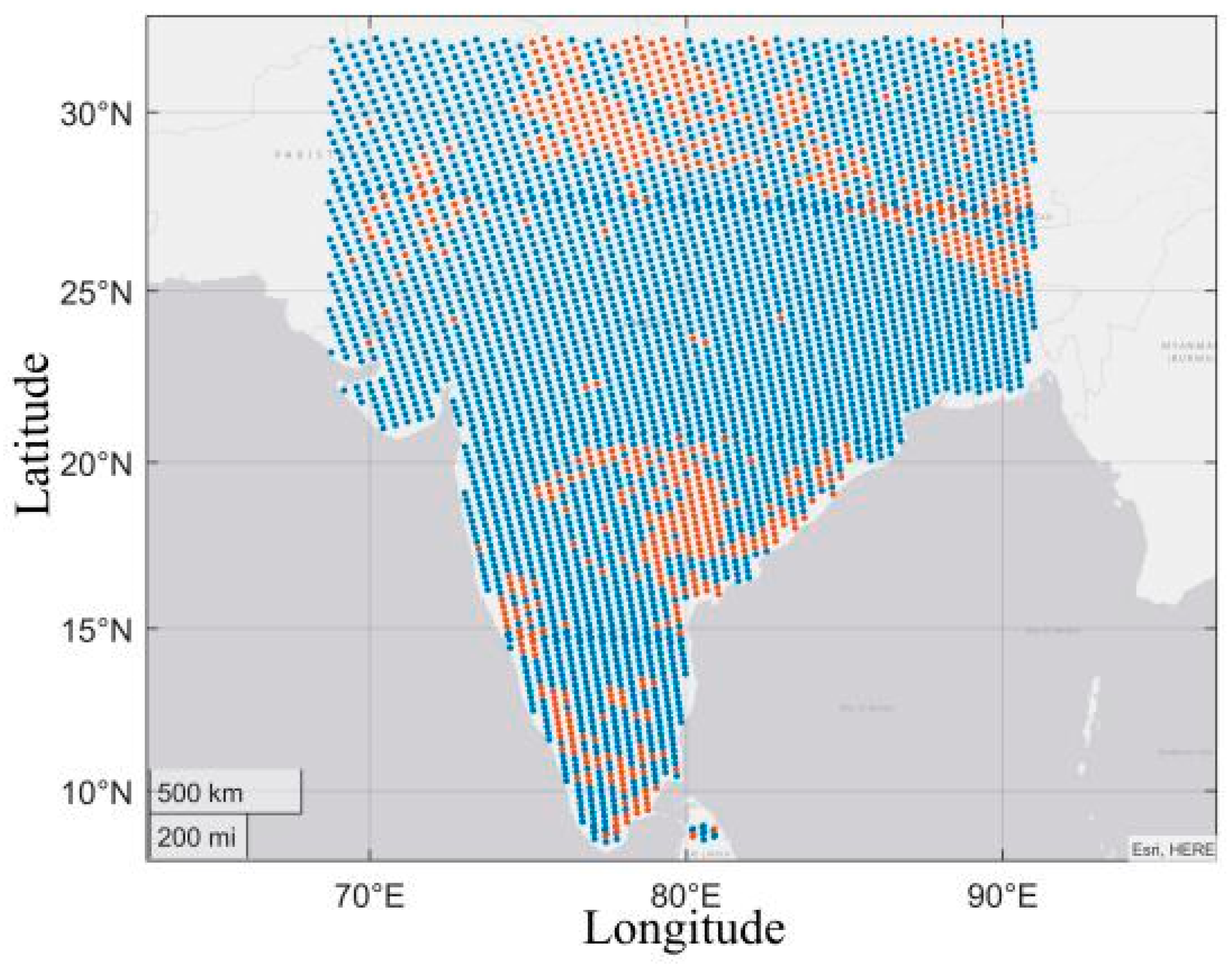
The data used for model training was mainly collected in India on 1–6 August 2019 and 1–3 February 2020 respectively. Figure 2 shows the location of the data set utilized for training from 00:30 to 01:30 on 1 February. Its longitude range is approximately 68.7°E–91°E while the latitude range is mainly in the land area of 8.4°N–32°N. In particular, the blue point refers to the selected clear sky pixel, and the red point refers to the abandoned cloud pixel.

3.3. ANN Retrieval Algorithm

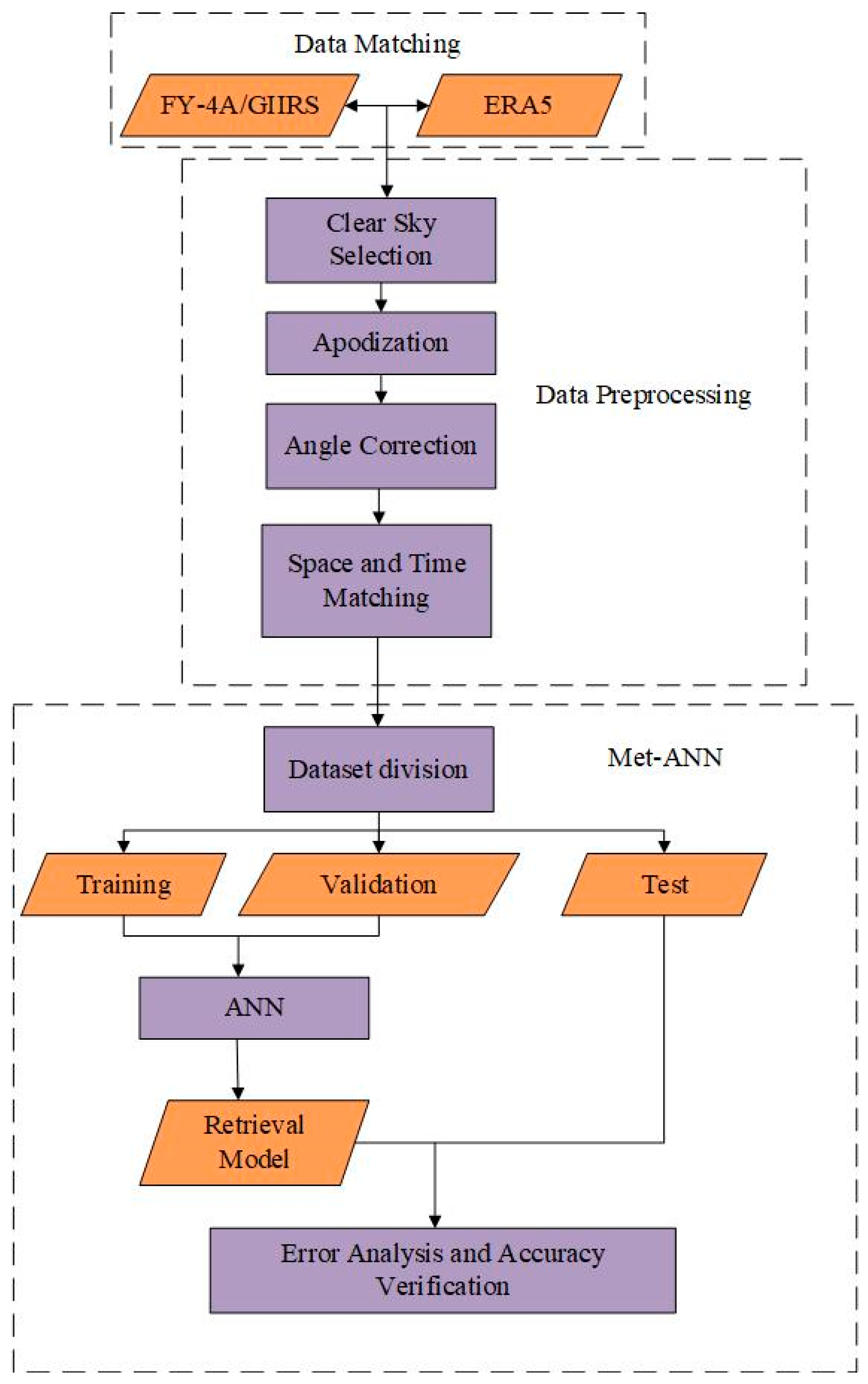
This section mainly introduces the principle and process of the ANN retrieval algorithm (Met-ANN). The process is shown in Figure 3. Data preprocessing (see Section 3.2) was performed on level L1 observation data (FY-4A/GIIRS) and reanalysis data (ERA5). We considered the influence of the satellite zenith angle on observation data, the radiance of each channel of each sample is multiplied by the cosine of the zenith angle of the satellite [22]. To be specific, the input layer was the observed brightness temperature of all channels (1650 neurons in total), and the target output layer was the temperature profile data of all pressure levels (37 neurons in total) [34]. The learning rate was 0.05. We randomly divided the dataset into 70%, 15%, and 15% as the training set, validation set, and test set respectively. We built an ANN training model, set the number of hidden layers to 1, and the determination of the number of hidden neurons mainly referred to in the article [35]. The author found that the number of hidden neurons obtained by the empirical Equation (9) was consistent with most application examples.
h = 0.43 n m + 0.12 m 2 + 2.54 n + 0.77 m + 0.35 + 0.51 ,
In Equation (9), n is the number of neurons in the input layer, m is the number of neurons in the output layer, and h (an integer by rounding up) is the number of neurons in the hidden layer.

3.4. Improved 1D-Var Retrieval Method

As shown in Figure 4, this section mainly introduces the principle and process of the improved 1D-Var retrieval algorithm (Met-I1DVar), at the same time introducing the method for establishing the channel blacklist, and the proposed strategy for error correction of observation data through ANN.

3.4.1. Covariance of Priori Error and Covariance of Observation Error

We preprocessed the L1 observation data (FY-4A/GIIRS), reanalysis data (ERA5), and forecast data (GFS) (see Section 3.2). We brought the reanalysis data in the RTTOV model to obtain the simulated brightness temperature/radiance. We then calculated the priori error covariance and the observation error covariance. The priori error covariance S a p was obtained from the deviation statistics of the GFS forecast data and the ERA5 reanalysis data, in the form of:
S a p = ( s 11 s 1 j s i 1 s i j ) ,
Specific calculations are shown in Equation (11):
s i j = cov ( x i , x j ) = 1 n k = 1 n [ ( x k i E ( x i ) ) ( x k j E ( x j ) ) ] ,
In Equation (11), s i j represents the priori error, x k i is the k -th sample data of the i -th level; E ( x i ) is the average error of the forecast value of the i -th level; n is the total number of samples.
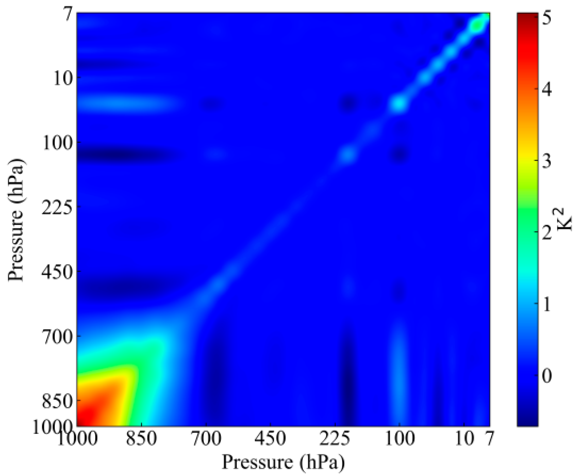
Figure 5 shows the covariance of temperature priori error. We considered the selected channels to be approximately independent. The observation error covariance matrix S ε is a diagonal matrix, and its diagonal elements are:
ε = ( Y m F ( x ) ) 2 n 1 ,
In Equation (12), m represents the number of channels. Y m is the observed brightness temperature of FY-4A/GIIRS, F ( x ) is the simulated brightness temperature calculated using the RTTOV forward model and reanalysis data x, and n is the number of samples.

3.4.2. Creating the Channel Blacklist

We selected the matched FY-4A/GIIRS and reanalysis profile data, and brought the true value profile, underlying surface, and angle data in the RTTOV model to obtain the simulated observation brightness temperature. We compared the simulated observed brightness temperature with the actual observed brightness temperature, and then analyzed the RMSE, which was caused by both the observation error and transfer model error (https://nwp-saf.eumetsat.int/downloads/rtcoef_rttov13/visir_lbl_comp/lbl_comp_rtcoef_fy4_1_giirs_v7pred_101L.html). The observation error analysis was carried out for each channel to find out the channel where the observation error was significantly greater than that of the adjacent channel, and the blacklist of the observation channel was established to screen the observation data.
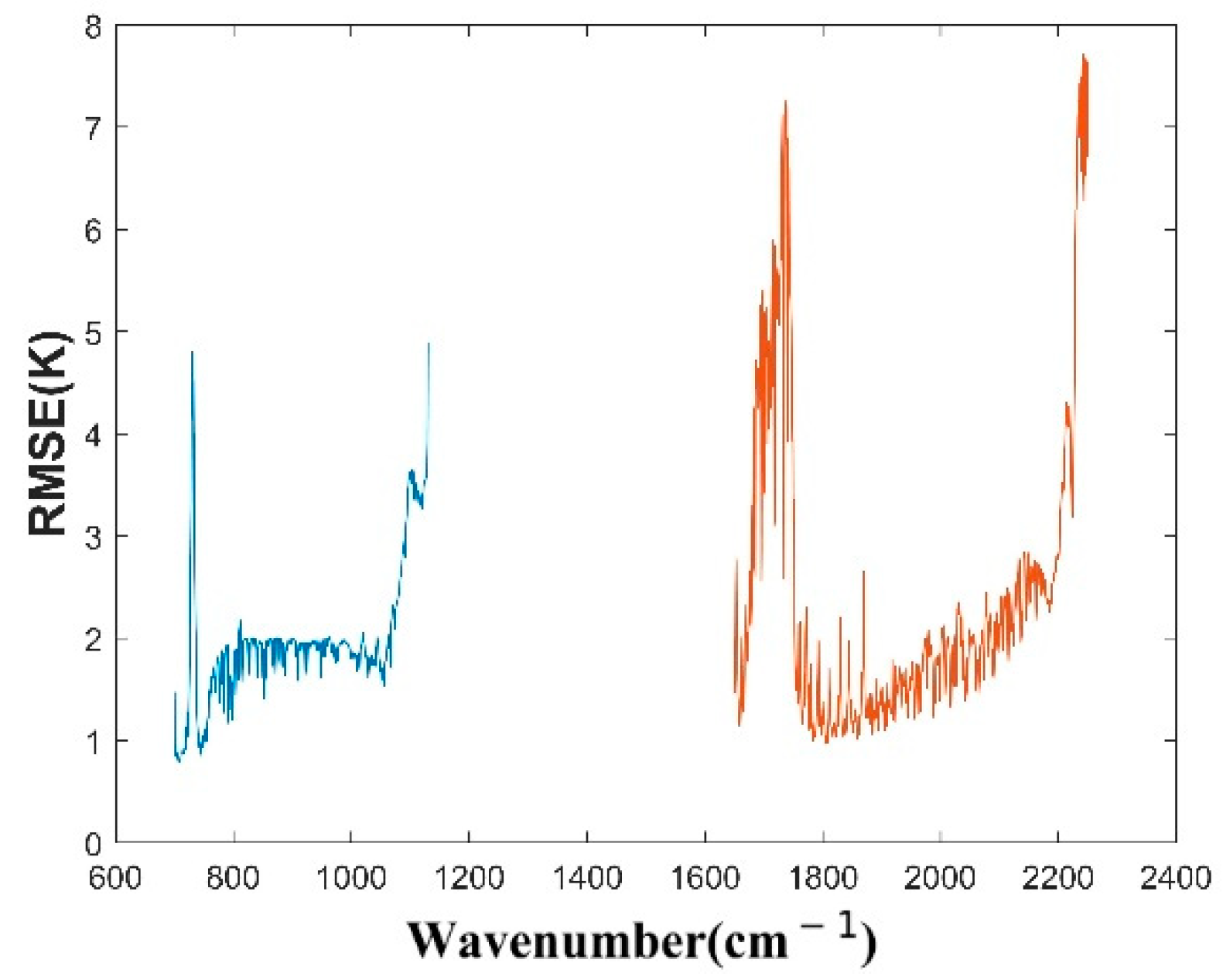
After data preprocessing, we randomly selected 30,000 sets of matching data, brought the reanalysis data in the RTTOV radiative transfer model to obtain the simulated brightness temperature, and calculated the RMSE between the simulated brightness temperature of each channel and the satellite observation brightness temperature. The statistical results are shown in Figure 6. After analysis, the blacklist of channels (235 channels in total) included a wave number range of: 726.25~735.625 cm−1 (RMSE was greater than 2 K), 1067.5~1130 cm−1 (RMSE was greater than 2 K), 1680~1753.125 cm−1 (RMSE was greater than 3 K). Since it was very important for retrieval temperature that the wave numbers were between 2200 cm−1 and 2250 cm−1, these channels were not included in the blacklist. In the following retrieval experiment, these channels were directly eliminated to reduce the influence of the errors in the data and the forward model.

3.4.3. Channel Selection

In our retrieval experiment, the more channels selected was not necessarily better. Selecting too many channels would introduce errors that interfered with the accuracy of the retrieval, leading to an increase in the retrieval error [36]. When the influence of information increase was greater than the influence of error increase, the retrieval error decreased; otherwise, the retrieval error increased.
Entropy can represent the uncertainty of information. In Equation (13), assuming that the probability distribution of vector x was a Gaussian distribution, S ^ is the error covariance matrix of state vector x, the information entropy C is defined as:
C [ P ( x ) ] = 1 2 log | S ^ | ,
In Equation (14), H is the difference of information entropy before and after retrieval, which is defined as the information capacity contained in satellite observation:
H = C [ P ( x ) ] C [ P ( x | Y ) ] = 1 2 log ( S ^ S a p 1 ) ,
In the FY-4A/GIIRS retrieval process, the column vectors of the atmospheric state constitute the vector x, the priori error covariance matrix is S a p , the error covariance matrix of retrieval parameters is S ^ , and K is the Jacobian matrix. The estimate of S ^ is as follows:
S ^ = S a p S a p K T ( K S a p K T + S ε ) 1 K S a p ,
S ^ 1 = ( K S ε K T + S a p ) 1 ,
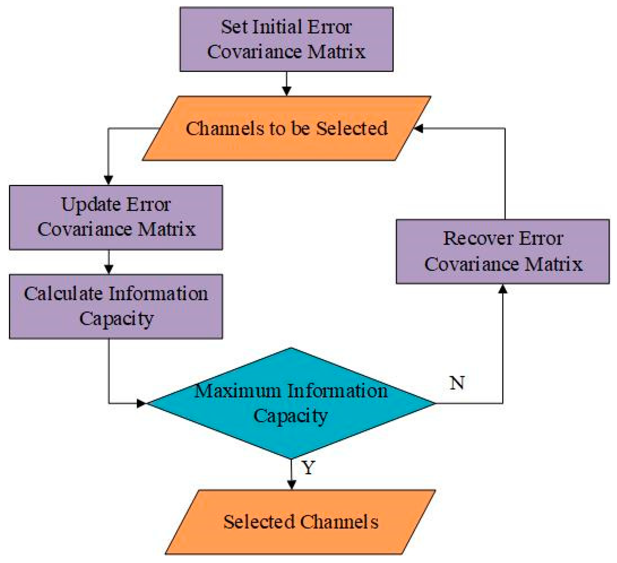
We combined the literature [37] to set the channel selection plan. We set the initial error covariance matrix S ^ to S a p . Figure 7 shows the process of one iteration. One channel was selected from the standby channels when making iteration per time, and the error covariance matrix S ^ and information capacity H were updated according to Equations (14)–(16). After traversing all the standby channels, the channel with the maximum information capacity was selected as the channel for this iteration. In total, 41 iterations were made for the temperature channel selection experiment.

3.4.4. Use ANN to Correct Observation Data

Regarding actual retrieval iterations, the main source that affected the final retrieval result was the error between the brightness temperature simulated by the forward radiative transfer model and the brightness temperature observed by the satellite. This error included both the radiative transfer model error and the satellite observation error. The correction of observation data in the original 1D-Var retrieval method only considered the satellite observation error. Our aim was to make the corrected satellite observations more similar to the simulated values of the transfer model.
Aimed at the shortcomings of the above physical methods, our FY-4A/GIIRS retrieval method introduced the ANN method to correct spectral data from satellite observations. In 11,695 matching sets of data, we brought the reanalyzed profile data, underlying surface and angle data in the RTTOV radiative transfer model to obtain the simulated brightness temperature. The satellite’s observed brightness temperature (excluding the channel in the blacklist) was used as the input sample of the training neural network, and the corresponding simulated brightness temperature (the channel for 1D-Var retrieval algorithm) was used as the training target output sample. The number of hidden neurons is as Equation (9).
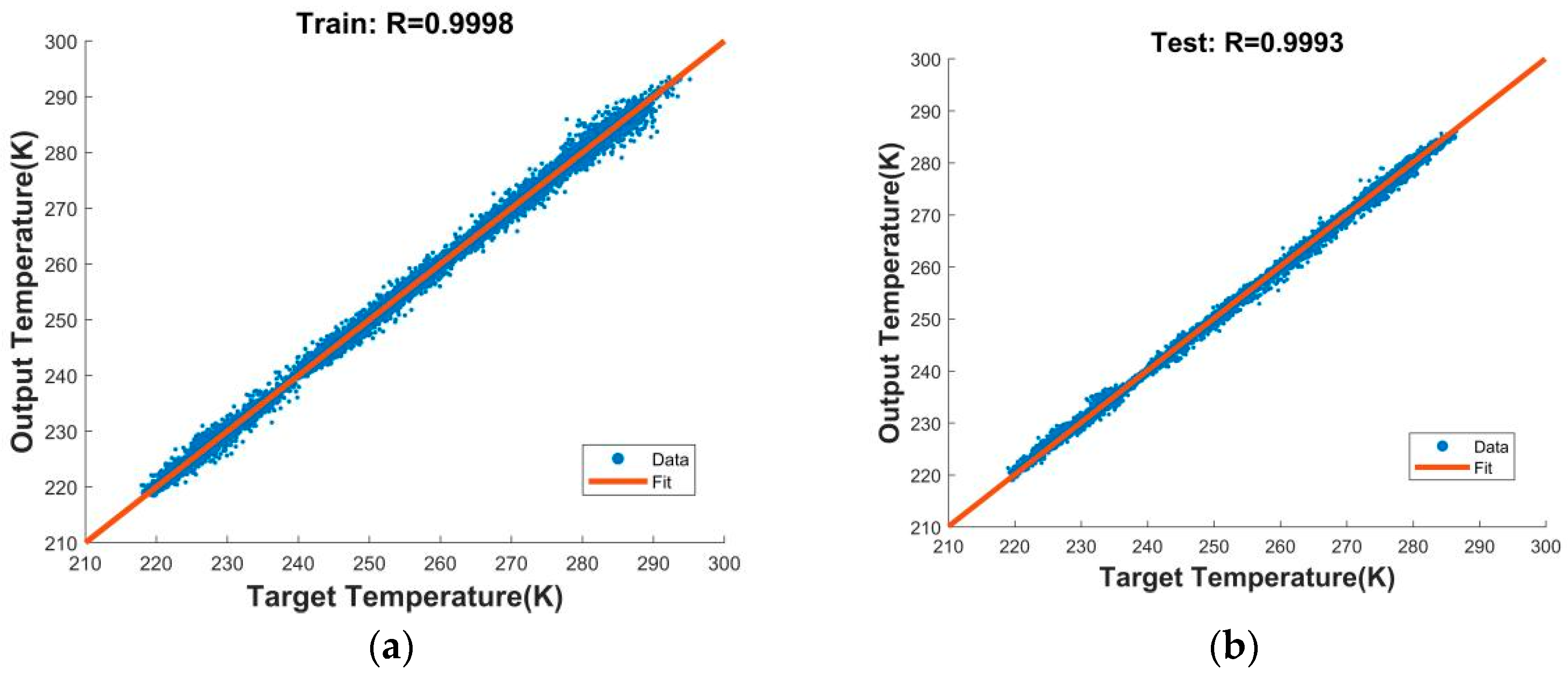
As shown in Figure 8, the horizontal axis of the figure was the target output brightness temperature (T), and the vertical axis was the output brightness temperature of the network (Y). Each group of samples was dotted with a blue dot on the figure according to its own T and Y. The closer the line Y = T was, the better the result of the network training was. We set the correlation coefficient R as an index to evaluate the quality of the model training. The R of the training set was 0.9998, and the R of the test set was 0.9993. From the analysis of the experimental test results, the network trained in this experiment was good and could be used for error correction of observation data.

3.4.5. Building an Objective Function

In this section, we used Newton’s non-linear iterations to minimize the objective function and obtain the temperature profiles. The objective function J [38,39,40,41] was defined as:
J ( x ) = 1 2 [ ( Y m F ( x ) ) T S ε 1 ( Y m F ( x ) ) ] + 1 2 [ ( x x b ) T γ S a p 1 ( x x b ) ] ,
In Equation (17), γ is the Lagrange smoothing factor, F ( x ) is the simulated observation from the forward radiative transfer model, S ε is the observation error covariance matrix, m is the number of channels involved in retrieval experiment, Y m and F ( x ) are both m dimensions, and x b is the priori field.
The final iteration equation is described as follows:
x n + 1 = x b + ( γ S a p 1 + K n T S ε 1 K n ) 1 K n T S ε 1 { [ Y m F ( x n ) ] + K n ( x n x b ) } ,
In Equation (18), n is the number of iterative times, x n + 1 and x n are the profile results of the (n + 1)-th and the n-th respectively, the initial x is derived from the GFS forecast profile, F ( x n ) is the brightness temperature obtained from forward transfer model in the n-th iteration, and K n is the Jacobian matrix calculated in the n-th iteration. The convergence condition is defined as Equation (19).
| x n + 1 x n | 2 < 0.05 ,
At the same time, the influence of the observation information and priori information on the solution was adjusted. The smaller γ was, the greater the influence of observed information would be; and inversely the greater the influence of priori information would be. The smooth factor γ was initially set to 1.
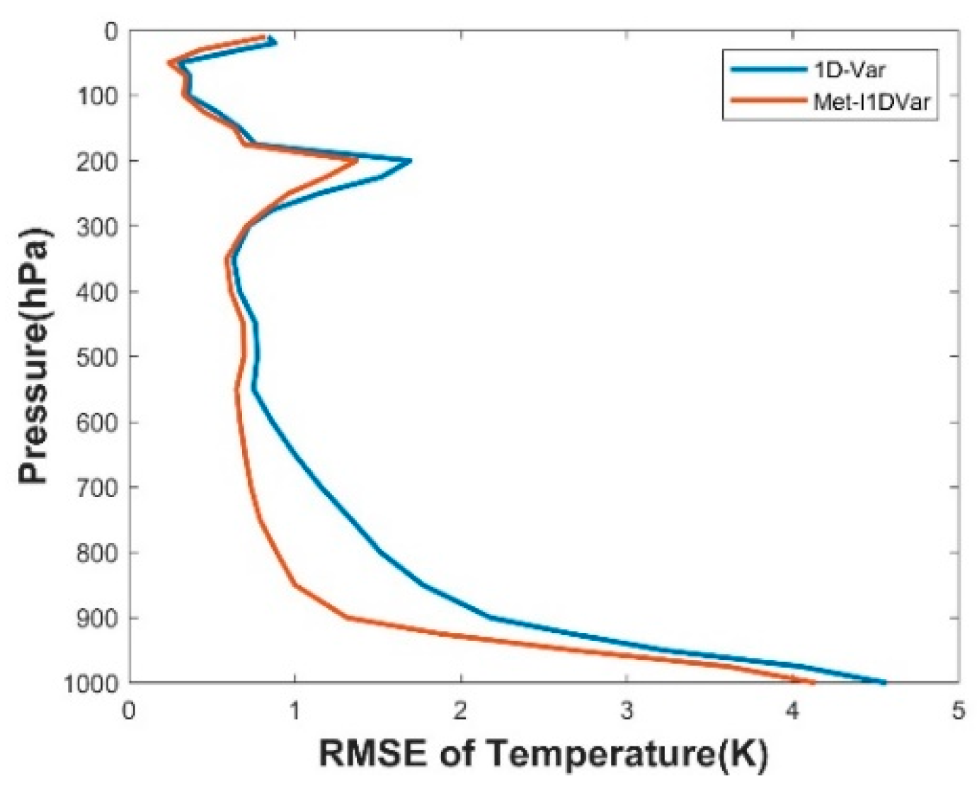
We randomly selected 1000 sets of preprocessed data from 1–6 August 2019 for comparison experiments. We defined Met-I1DVar, apart from ’Create Channel Blacklist’ and ’Use ANN to Correct Observation Data’, as the conventional 1D-Var. We used the conventional 1D-Var and Met-I1DVar to retrieve the temperature, respectively. As shown in Figure 9, we calculated the RMSE of the retrieval temperature profiles of two methods based on the reanalysis temperature profiles, respectively. From the statistical results of RMSE, Met-I1DVar had an obvious advantage over the conventional 1D-Var retrieval algorithm. The RMSE of Met-I1DVar was less than 1 K in the 10 hPa–200 hPa and 300 hPa–800 hPa pressure levels. The results showed that the accuracy of profile retrieval could be effectively improved by establishing a channel blacklist and introducing ANN for observation data correction.

3.5. Construct an Improved FY-4A/GIIRS Retrieval Method

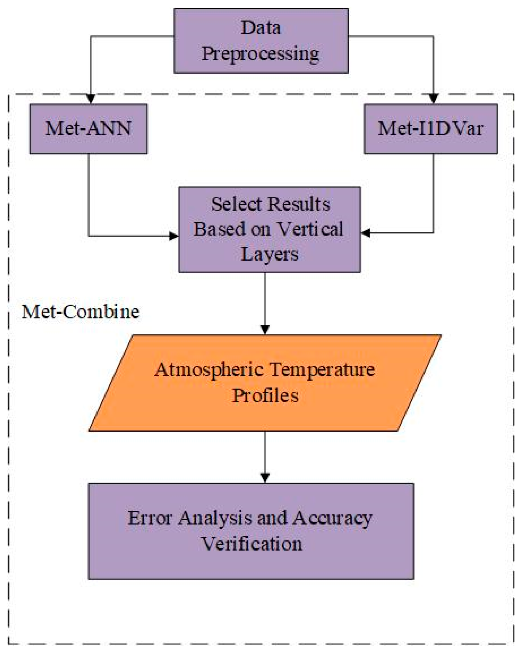
After data preprocessing (see Section 3.2), ANN (see Section 3.3) and improved 1D-Var (see Section 3.4) were respectively used for the retrieval experiment. Since there were significant differences between the accuracy of some pressure levels for the two algorithms, after theoretical analysis of the algorithm and statistical results of a large number of experiments, we selected the appropriate algorithm for retrieval according to their different pressure levels, defining our method as Met-Combine. Finally, we carried out error analysis and accuracy evaluation. Figure 10 shows the process of Met-Combine.
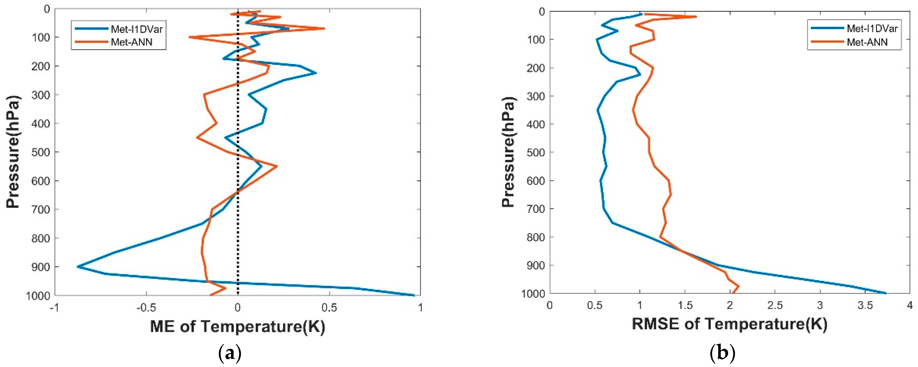
We selected 1000 sets of data from all samples for testing (1–6 August 2019 and 1–3 February 2020), and calculated RMSE and ME from the retrieval results of the two methods based on the reanalysis data respectively, then compared the retrieval accuracy of Met-ANN and Met-I1DVar. The relevant results are shown in Figure 11. Met-I1DVar had a larger RMSE at 800 hPa–1000 hPa near the surface, while the RMSE of the remaining pressure levels was smaller than Met-ANN.
Finally, we built an improved temperature retrieval method based on the above retrieval results and theoretical analysis. In temperature retrieval experiments, Met-ANN was used at the pressure levels of 800 hPa–1000 hPa, while Met-I1DVar was selected for the remaining pressure levels.

4. Results

4.1. Test Data

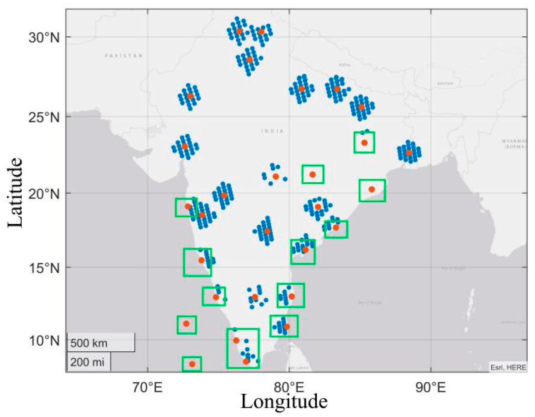
Our experiment data was selected in India, the training data of which was from 1–3 February 2020; and the test data of which was from 4–10 February 2020 at 00:00UTC. Figure 12 shows the sounding data (red dot) and GIIRS observation data (blue dot) used for testing at 0:00 on 4 February. GFS forecast data was interpolated and matched with GIIRS observation data through the linear interpolation method, as described in Section 3.2. We allocated GIIRS observation data points and sounding data points through the conditions specified in Equation (20). If the number of blue dots nearby red dots was less than 4, or these blue dots were generally located to one side, we would delete the data. The green box in the figure contains the sounding data points we deleted. There were altogether 118 sets of sounding data used for testing on 4–10 February 2020. After retrieving the temperature profiles, the profile data and sounding data were also interpolated temporally and spatially as per the interpolation method described in Section 3.2. Sounding data was taken as the true value in this experiment to evaluate the accuracy of the temperature profile retrieval method. In Equation (20), l a t 1 and l o n 1 represent the latitude and longitude of the observation data, respectively. l a t 0 and l o n 0 represent the latitude and longitude of the sounding data, respectively.
| l a t 1 l a t 0 | + | l o n 1 l o n 0 | < 1 ° ,

4.2. Correction of Observation Data

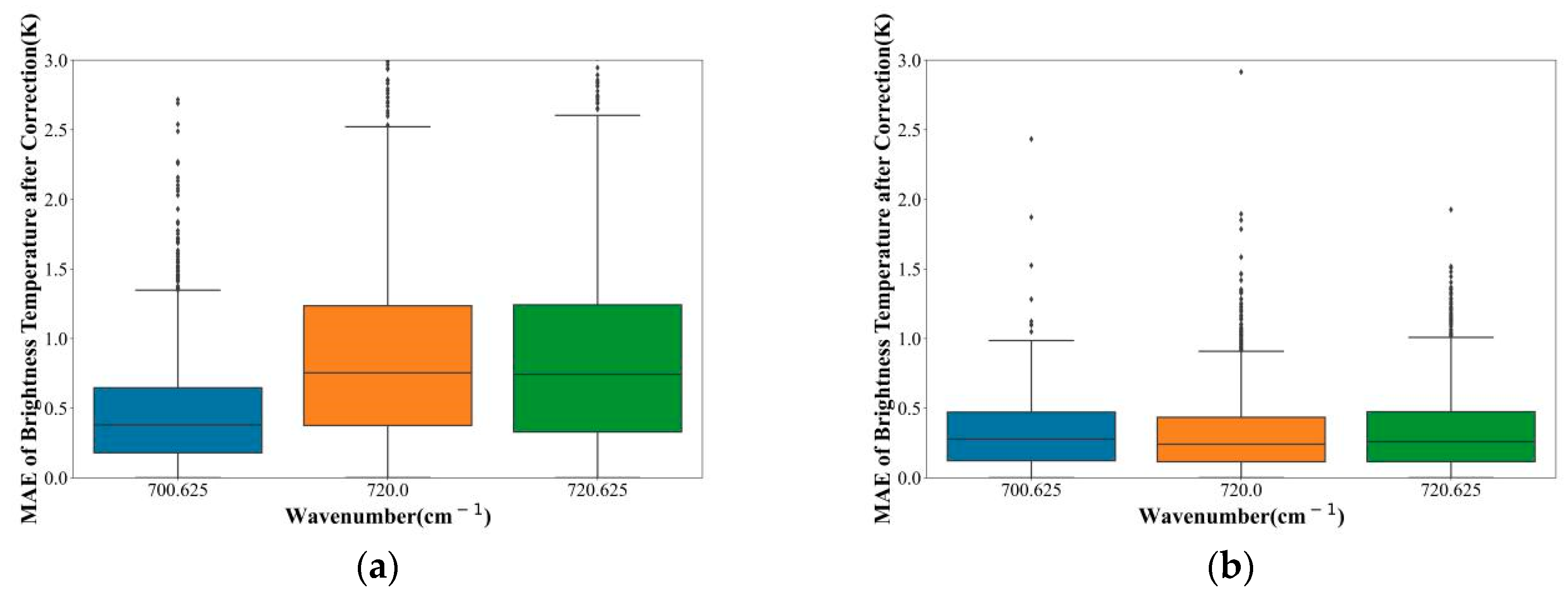
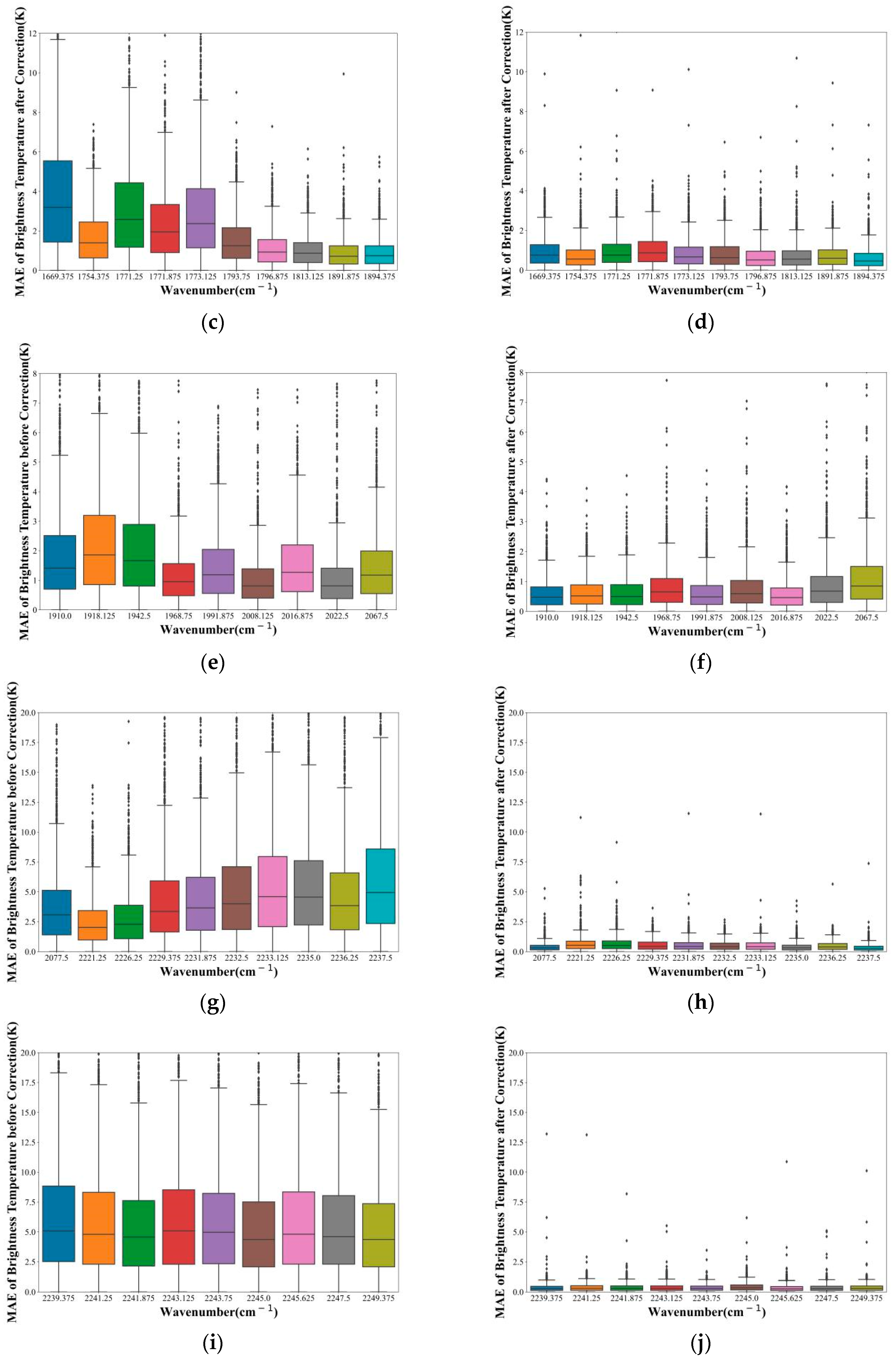
The training data was collected from the whole of the Indian region on 1–3 February. The simulated brightness temperature was obtained by substituting the reanalysis data into RTTOV. The error of the observed brightness temperature of the channel selected was also corrected as per the method in Section 3.4.4. See Section 4.1 for the descriptions of test data. Statistics on the MAE of the observed brightness temperature and the simulated brightness temperature of the test set before and after correction were made.
As shown in Figure 13, the MAE of all selected channels after correction was less than that before correction. Additionally, the MAE of most corrected channels was less than 0.5 K. We could find a trend: the greater the wave number, the more obvious the correction effect of the channel. Using the ANN method to correct the error of the observation data of the selected channel could effectively reduce the error of the observation data and the forward model.

4.3. Compare the Retrieval Results of Met-ANN with Met-I1DVar

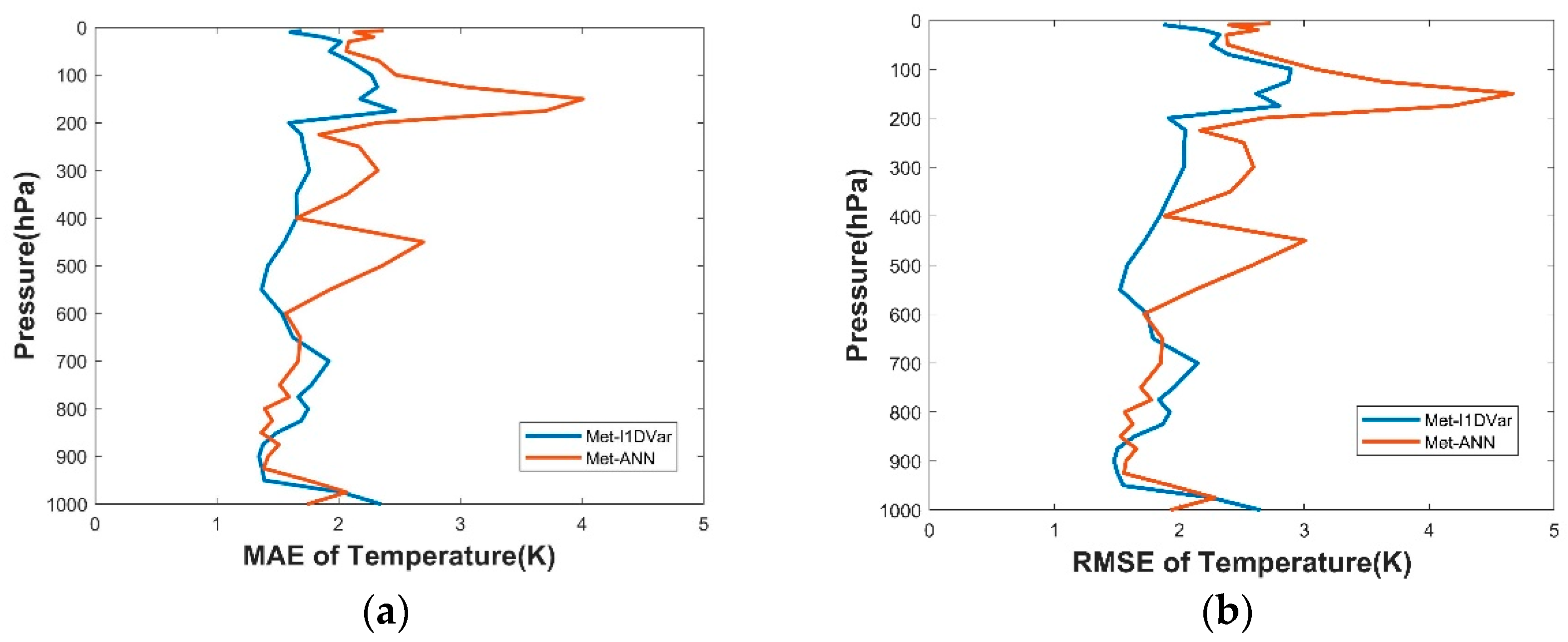
As shown in Section 4.1, where the test data was introduced, we utilized Met-ANN and Met-I1DVar to retrieve the temperature profiles, and took the sounding data as the true value, so as to statistically analyze the MAE and RMSE of temperature profiles retrieved by using the two methods. As shown in Figure 14, MAE and RMSE showed basically the same variation error curve. The error with Met-ANN was smaller than that with Met-I1DVar from 650 hPa to 850 hPa and from 975 hPa to 1000 hPa, respectively and the error with Met-I1DVar was smaller than that with Met-ANN in other atmospheric pressure levels. The error of the two methods had little difference between 600 hPa and 1000 hPa. However, Met-ANN was advantageous over Met-I1DVar between 10 hPa–600 hPa.

4.4. Compare the Retrieval Results of Met-Combine with GIIRS Products

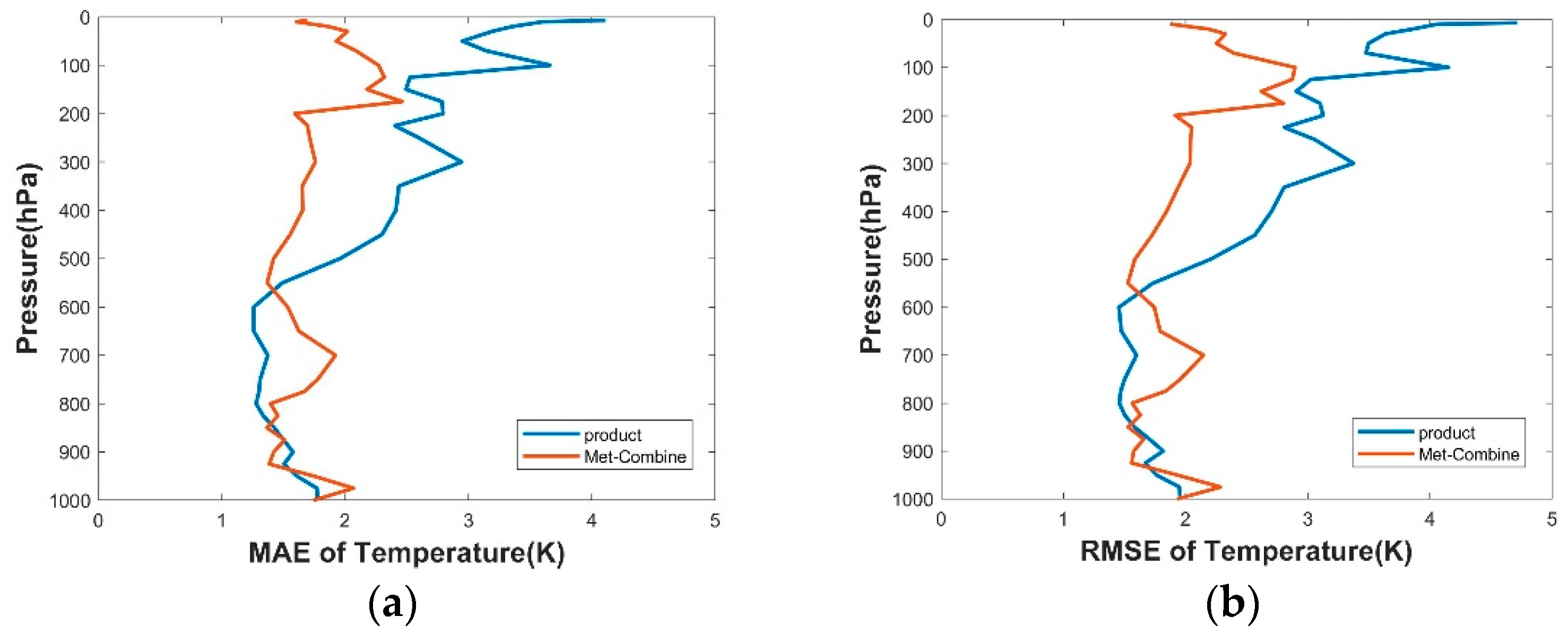
The test method was introduced in Section 4.1. Statistics on MAE and RMSE of Met-Combine and GIIRS temperature profile products were made. As shown in Figure 15, the variation error curves of MAE and RMSE were basically the same. The error of the GIIRS product was smaller than that with Met-Combine from 575 hPa to 850 hPa and from 925 hPa to 1000 hPa, while that with Met-Combine was smaller than that of GIIRS product in other atmospheric pressure levels. The error of the GIIRS product was smaller than 2 K in general between 525 hPa and 1000 hPa. The average error with Met-Combine was smaller than that of the GIIRS product, between 10 hPa and 1000 hPa.

5. Discussion

Taking the reanalysis data of ERA5 as a basis, we adopted the ANN method to correct the selected observation data for temperature retrieval. The corrected errors of almost all channels are lower than those made before correction, and the MAE among the corrected observed brightness temperatures of most channels and those simulated can be lower than 0.5 K. The reanalysis data of ERA5 features high temporal and spatial resolution with high accuracy, the data of which can be collected almost anywhere in the world, which is very suitable for ANN training as a basis. The network inputs are the observed brightness temperatures of all channels excluded in the blacklist. A large number of channels will be abandoned in the subsequent retrieval test. However, these abandoned channels provide the observation information during brightness temperature correction, so Met-I1DVar (see Section 3.4) effectively improves the utilization rate of the observation information.
We compared the accuracy of Met-ANN (see Section 3.3) with that of Met-I1DVar for temperature retrieval. In Section 3.5, we selected some data sets for training based on ERA5 data to perform the temperature retrieval tests. According to the ME and RMSE results of the two methods, we found that the accuracy of Met-ANN from 800 hPa to 1000 hPa is higher than that of Met-I1DVar, and the accuracy of other pressure levels is lower than that of Met-I1DVar. In Section 4.3, we adopted Met-ANN and Met-I1DVar based on the sounding data published by the University of Wyoming to perform temperature retrieval tests on the test data sets and compiled statistics on the MAE and RMSE results. We found that Met-ANN is better from 600 hPa to 1000 hPa, while Met-I1DVar is obviously better in other levels. In both tests, we found that the accuracy of Met-ANN is higher than that of Met-I1DVar in pressure levels near the ground, and Met-I1DVar is much better in pressure levels further away from the ground.
In Section 4.4, we compared the accuracy of temperature profiles retrieved by Met-Combine (see Section 3.5) based on the sounding data published by the University of Wyoming in early February 2020 in India with that of temperature profile products obtained by GIIRS. We found that the temperature profile products obtained by GIIRS in some pressure levels (such as 10 hPa–500 hPa and 850 hPa–925 hPa) can be improved. As a load on GEO satellites, GIIRS has a higher temporal resolution and can provide a large number of samples for ANN training. Met-Combine provides the advantages of machine learning and can effectively extract more observation information than using physical methods.
However, Met-Combine has some shortcomings:
(1).
From 550 hPa to 800 hPa, the accuracy of temperature profiles retrieved according to Met-Combine is lower than that of temperature profile products obtained by GIIRS. The method in this paper is applicable to Ver. V3 of GIIRSL1 data.
(2).
In Met-Combine, the retrieval results of different pressure levels obtained by the above mentioned two methods are combined together, which may cause inconsistent sensitivity. We layered the atmosphere vertically according to the atmospheric pressure so that the retrieved profiles are discrete, and then we output profiles with a higher vertical resolution by fitting. This method is helpful for reducing the influence of inconsistent sensitivity. In addition, we believe that the error (such as RMSE) between a retrieved profile and the true value is more noticeable than inconsistent sensitivity. Therefore, the inconsistent sensitivity of profiles in different pressure levels caused by the combined methods does not influence the availability of data.
(3).
Met-Combine also has the same shortcomings as encountered in the ANN method. For example, incomplete training samples may cause bad retrieval effects on some test data, and complicated steps regarding the training coefficient will lead to a relatively long model training time, in addition, data quality for training is hard to control. Therefore, whether Met-Combine can be adopted in practice and obtain better retrieval results still needs further verification.

6. Conclusions

In this paper, the 1D-Var retrieval algorithm (see Met-I1DVar in Section 3.4) is improved. A comparison test of temperature profile retrieval between the improved 1D-Var algorithm and ANN algorithm (see Met-ANN in Section 3.3) based on the GIIRS data observed in India in early February was performed. We found that the ANN retrieval algorithm is more suitable for the temperature retrieval of pressure levels near the ground, while the 1D-Var algorithm is more suitable for pressure levels further away from the ground. By combining Met-ANN and Met-I1DVar, a retrieval method suitable for retrieving atmospheric temperature profiles based on the GIIRS observation data (see Met-Combine in Section 3.5) was proposed. Using the GIIRS data observed in India in early February, the error of temperature profiles retrieved according to Met-Combine and the error of temperature profile products obtained by GIIRS were recorded. For some pressure levels, the accuracy of the temperature profiles that were retrieved according to Met-Combine is higher than that of GIIRS temperature profile products. We found that Met-Combine is more suitable for improving the accuracy of GIIRS temperature profile products at 10 hPa–500 hPa and 850 hPa–925 hPa.
Compared with the ANN retrieval algorithm, Met-Combine introduces the priori information of forecast data and effectively adopts the observation information of underlying surfaces and satellites; compared with the traditional 1D-Var retrieval algorithm, Met-Combine can extract more channel observation information, reduce errors from the radiative transfer model and satellite observation and effectively use the observation information of 1415 channels combined with the characteristics of FY-4A/GIIRS observation data. Therefore, the accuracy of Met-Combine is higher than the other two methods.
GIIRS is a load on GEO Satellite FY-4A, which is the first infrared hyperspectral detector on the geostationary orbit. Compared with other similar instruments, it has an obviously higher time resolution. In a short period of time, GIIRS can provide a large amount of observation data for the same area, which is very suitable for training machine learning models. This paper combines traditional physical retrieval methods with a machine learning method, which can provide a reference for improving the accuracy of products. We can improve the utilization rate of the GIIRS observation information by improving the retrieval method. In short, we believe that the GEO satellite-based infrared hyperspectral detection technology has broad development prospects.

Author Contributions

Conceptualization, P.H. and Q.G.; methodology, P.H.; software, P.H.; validation, P.H., C.Z., T.Y. and S.H.; formal analysis, P.H.; investigation, C.Z.; resources, C.H.; data curation, Q.G.; writing—original draft preparation, C.Z. and P.H.; writing—review and editing, P.H., C.Z., Q.G. and C.H.; visualization, Q.G.; supervision, Q.G.; project administration, Q.G. All authors have read and agreed to the published version of the manuscript.

Funding

This research was funded by National Natural Science Foundation of China (41875037).

Data Availability Statement

All data generated or analyzed during this study are included in this article.

Acknowledgments

We would like to thank the NSMC (National Satellite Meteorological Center) for sharing FY-4A/GIIRS data. Meanwhile we also would like to thank Yong Hu and Mingjian Gu of Shanghai Institute of Technical Physics, Chinese Academy of Sciences for our equipment resources and technical guidance. We are very grateful to Di di of Nanjing University of Information Science and Technology for manuscript writing guidance. Finally, we would like to thank Huangwei Tu, Haifei Zeng and Xin Liu of Shanghai Institute of Technical Physics, Chinese Academy of Sciences for their contributions to data processing methods and encouragement to us.

Conflicts of Interest

The authors declare no conflict of interest.

References

  1. Guan, Y.H.; Ren, J.; Bao, Y.S.; Lu, Q.F.; Liu, H.; Xiao, X.J. Research of the infrared high spectral (IASI) satellite remote sensing atmospheric temperature and humidity profiles based on the one-dimensional variational algorithm. Trans. Atmos. Sci. 2019, 42, 602–611. [Google Scholar]
  2. Von Clarmann, T.; Degenstein, D.A.; Livesey, N.J.; Bender, S.; Braverman, A.; Butz, A.; Compernolle, S.; Damadeo, R.; Dueck, S.; Eriksson, P.; et al. Overview: Estimating and reporting uncertainties in remotely sensed atmospheric composition and temperature. Atmos. Meas. Tech. 2020, 13, 4393–4436. [Google Scholar] [CrossRef]
  3. Dong, C.H.; Li, J.; Zhang, P. The Principle and Application of Satellite Hyperspectral Infrared Atmospheric Remote Sensing; Science Press: Beijing, China, 2013. [Google Scholar]
  4. Che, Y.; Ma, S.; Xing, F.; Li, S.; Dai, Y. An improvement of the retrieval of temperature and relative humidity profiles from a combination of active and passive remote sensing. Meteorol. Atmos. Phys. 2019, 131, 681–695. [Google Scholar] [CrossRef]
  5. Solheim, F.; Godwin, J.R.; Westwater, E.R.; Han, Y.; Keihm, S.J.; Marsh, K.; Ware, R. Radiometric profiling of temperature, water vapor and cloud liquid water using various inversion methods. Radio Sci. 1998, 33, 393–404. [Google Scholar] [CrossRef] [Green Version]
  6. Zhang, P.; Guo, Q.; Chen, B.Y.; Feng, X. The Chinese next-generation geostationary meteorological satellite FY-4 compared with the Japanese Himawari-8/9 satellite. J. Adv. Met. S T 2016, 6, 72–75. [Google Scholar]
  7. Chen, R.; Gao, C.; WU, X.W.; Zhou, S.Y.; Hua, J.W.; Ding, L. Application of FY-4 atmospheric verticals sounder in weather forecast. J. Infrared Millim. Waves 2019, 38, 285–289. [Google Scholar]
  8. Guo, Q.; Yang, J.; Wei, C.Y.; Chen, B.Y.; Wang, X.; Han, C.P.; Hui, W.; Xu, W.W.; Wen, R.; Liu, Y.N. Spectrum Calibration of the First Hyperspectral Infrared Measurements from a Geostationary Platform: Method and Preliminary Assessment. Q. J. R. Meteorol. Soc. 2021. [Google Scholar] [CrossRef]
  9. Chen, B.Y.; Wu, Q.; Feng, X.; Guo, Q.; Wei, C.Y. On-orbit test to FY-4A AGRI and generating RBG image. J. Infrared Millim. Waves 2018, 37, 411–415. [Google Scholar]
  10. Luo, S.; Di, D.; Cui, L.L. Study on FY-4A/GIIRS infrared spectrum detection capability based on information content. J. Infrared Millim. Waves 2019, 38, 765–776. [Google Scholar]
  11. Menzel, W.P.; Schmit, T.J.; Zhang, P.; Li, J. Satellite-Based Atmospheric Infrared Sounder Development and Applications. B Am. Meteorol. Soc. 2018, 99, 583–603. [Google Scholar] [CrossRef]
  12. Guan, L. Retrieving Atmospheric Profiles from MODIS/AIRS Observations. I. Eigenvector Regression Algorithms. J. Nanjing Inst. Meteorol. 2006, 6, 756–761. [Google Scholar]
  13. Jiang, D.M.; Dong, C.H.; Lu, W.S. Preliminary Study on the Capacity of High Spectral Resolution Infrared Atmospheric Sounding Instrument Using AIRS Measurements. J. Remote Sens. 2006, 10, 586–592. [Google Scholar]
  14. Zhang, J.; Li, Z.L.; Li, J.; Li, J.L. Ensemble Retrieval of Atmospheric Temperature Profiles from AIRS. Adv. Atmos. Sci. 2014, 31, 559–569. [Google Scholar] [CrossRef]
  15. Ma, P.F.; Chen, L.F.; Tao, J.H.; Su, L.; Tao, M.H.; Wang, Z.F.; Hao, M.M.; Zhang, Y. Study on Simulation of infrared hyperspectral CrIS data retrieval of atmospheric temperature and humidity profiles. J. Spectrosc. Spectr. Anal. 2014, 07, 1894–1897. [Google Scholar]
  16. Shi, L.; Matthews, J.L.; Ho, S.-P.; Yang, Q.; Bates, J.J. Algorithm development of temperature and humidity profile retrievals for long-term HIRS observations. Remote Sens. 2016, 8, 280. [Google Scholar] [CrossRef] [Green Version]
  17. Blackwell, W.J. A neural-network technique for the retrieval of atmospheric temperature and moisture profiles from high spectral resolution sounding data. IEEE Trans. Geosci. Remote Sens. 2005, 43, 2535–2546. [Google Scholar] [CrossRef]
  18. Zheng, G.; Yang, J.S.; Li, X.F.; Zhou, L.Z.; Ren, L.; Chen, P.; Zhang, H.G.; Lou, X.L. Using artificial neural network ensembles with crogging resampling technique to retrieve sea surface temperature from hy-2a scanning microwave radiometer data. IEEE Trans. Geosci. Remote Sens. 2018, 57, 985–1000. [Google Scholar] [CrossRef]
  19. Milstein, A.B.; Blackwell, W.J. Neural network temperature and moisture retrieval algorithm validation for AIRS/AMSU and CrIS/ATMS. J. Geophys. Res. Atmos. 2016, 121, 1414–1430. [Google Scholar] [CrossRef] [Green Version]
  20. Yang, Y.; Shen, F.; Yang, Z.C.; Feng, X.S. Prediction of Solar Wind Speed at 1 AU Using an Artificial Neural Network. Space Weather 2018, 16, 1227–1244. [Google Scholar] [CrossRef]
  21. Cabreramercader, C.R.; Staelin, D.H. Passive microwave relative humidity retrievals using feedforward neural networks. IEEE Trans. Geosci. Remote 2002, 33, 1324–1328. [Google Scholar]
  22. Cai, X.; Bao, Y.S.; Petropoulos, G.P.; Lu, F.; Zhu, L.H.; Wu, Y. Temperature and Humidity Profile Retrieval from FY4-GIIRS Hyperspectral Data Using Artificial Neural Networks. J. Remote Sens. 2020, 12, 1872. [Google Scholar] [CrossRef]
  23. Cimini, D.; Hewison, T.J.; Martin, L.; Güldner, J.; Gaffard, C.; Marzano, F.S. Temp. and humidity profile retrievals from ground-based microwave radiometers during TUC. J. Meteorologische Z. 2006, 15, 45–56. [Google Scholar] [CrossRef]
  24. Churnside, J.H.; Stermitz, T.A.; Schroeder, J.A. Temperature Profiling with Neural Network Inversion of Microwave Radiometer Data. J. Atmos. Ocean. Technol. 1994, 11, 105–109. [Google Scholar] [CrossRef] [Green Version]
  25. Duncan, D.I.; Kummerow, C.D. A 1DVAR retrieval applied to GMI: Algorithm description, validation, and sensitivities. J. Geophys. Res. Atmos. 2016, 121, 7415–7429. [Google Scholar] [CrossRef] [Green Version]
  26. Alvarado, M.J.; Payne, V.H.; Mlawer, E.J.; Uymin, G.; Shephard, M.W.; Cady-Pereira, K.E.; Delameres, J.S.; Moncet, J.L. Performance of the Line-By-Line Radiative Transfer Model (LBLRTM) for temperature, water vapor, and trace gas retrievals: Recent updates evaluated with IASI case studies. Atmos. Chem. Phys. 2013, 13, 6687–6711. [Google Scholar] [CrossRef] [Green Version]
  27. Shen, Z.X.; Liu, C.S. A study on the inversion of atmospheric temperature and humidity profiles by using CrIS infrared hyperspectral satellite data. J. East China Norm. Univ. 2019, 3, 199–210. [Google Scholar]
  28. Zhu, L.H.; Bao, Y.S.; Petropoulos, G.P.; Zhang, P.; Lu, F.; Lu, Q.F.; Wu, Y.; Xu, D. Temperature and Humidity Profiles Retrieval in a Plain Area from Fengyun-3D/HIRAS Sensor Using a 1D-VAR Assimilation Scheme. J. Remote Sens. 2020, 12, 435. [Google Scholar] [CrossRef] [Green Version]
  29. Hua, J.H.J.; Wang, Z.W.Z.; Duan, J.D.J.; Li, L.L.L.; Zhang, C.Z.C.; Wu, X.W.X.; Fan, Q.F.Q.; Chen, R.C.R.; Sun, X.S.X.; Zhao, L.Z.L.; et al. Review of Geostationary Interferometric Infrared Sounder. J. Chin. Opt. Lett. 2018, 16, 111203. [Google Scholar]
  30. Feng, X.; Li, L.B.; Chen, B.Y.; Zou, Y.P.; Han, C.P. Post-launch calibration and validation of the Geostationary Interferometric Infrared Sounder(GIIRS) on FY-4A. J. Infrared Millim. Waves. 2019, 38, 648–654. [Google Scholar]
  31. Yang, J.; Zhang, Z.Q.; Wei, C.Y.; Lu, F.; Guo, Q. Introducing the new generation of Chinese geostationary weather satellites FENGYUN-4. Bull. Amer. Meteor. Soc. 2018, 98, 1637–1658. [Google Scholar] [CrossRef]
  32. Di, D.; Li, J.; Han, W.; Bai, W.; Wu, C.; Menzel, W.P. Enhancing the Fast Radiative Transfer Model for FengYun-4 GIIRS by Using Local Training Profiles. J. Geophys. Res. Atmos. 2018, 123. [Google Scholar] [CrossRef]
  33. Yang, T.H.; Hu, X.Q.; Xu, H.L.; Wu, C.Q.; Qi, C.L.; Gu, M.J. Radiation Calibration Accuracy Assessment of FY-3D Hyperspectral Infrared Atmospheric Sounder Based on Inter-Comparison. Acta Optica Sin. 2019, 39, 377–387. [Google Scholar]
  34. Bao, Y.S.; Wang, Z.J.; Chen, Q.; Zhou, A.M.; Dong, Y.H.; Min, J.Z. Preliminary Study on Atmospheric Temperature Profiles Retrieval from GIIRS Based on FY-4A Satellite. Aerosp. Shanghai 2017, 34, 28–37. [Google Scholar]
  35. Gao, D.Q. On structures of supervised linear basis function feedforward three-layered neural networks. Chin. J. Comput. 1998, 21, 80–86. [Google Scholar]
  36. Rodgers, C.D. Information content and optimization of high spectral resolution remote measurements. Adv. Space Res. 1996, 21, 136–147. [Google Scholar]
  37. Yang, Y.H.; Yin, Q.; Shu, J. Channel selection of atmosphere vertical sounder (GIIRS) on board the FY-4A geostationary satellite. J. Infrared Millim. Waves 2018, 37, 545–552. [Google Scholar]
  38. Yang, J.; Min, Q. Retrieval of Atmospheric Profiles in the New York State Mesonet Using One-Dimensional Variational Algorithm. J. Geophys. Res. Atmos. 2018, 123, 7563–7575. [Google Scholar] [CrossRef]
  39. Jang, H.S.; Sohn, B.J.; Chun, H.W.; Li, J.; Weisz, E. Improved AIRS temperature and moisture soundings with local a priori information for the 1DVAR method. J. Atmos. Ocean. Technol. 2017, 34, 1083–1095. [Google Scholar] [CrossRef]
  40. Ishimoto, H.; Okamoto, K.; Okamoto, H.; Sato, K. One-dimensional variational (1D-Var) retrieval of middle to upper tropospheric humidity using AIRS radiance data. J. Geophys. Res. Atmos. 2014, 119, 7633–7654. [Google Scholar] [CrossRef]
  41. Martinet, P.; Dabas, A.; Donier, J.M.; Doffer, T.; Garrouste, O.; Guillot, R. 1D-Var temperature retrievals from microwave radiometer and convective scale model. Tellus A 2015, 67, 27925. [Google Scholar] [CrossRef] [Green Version]
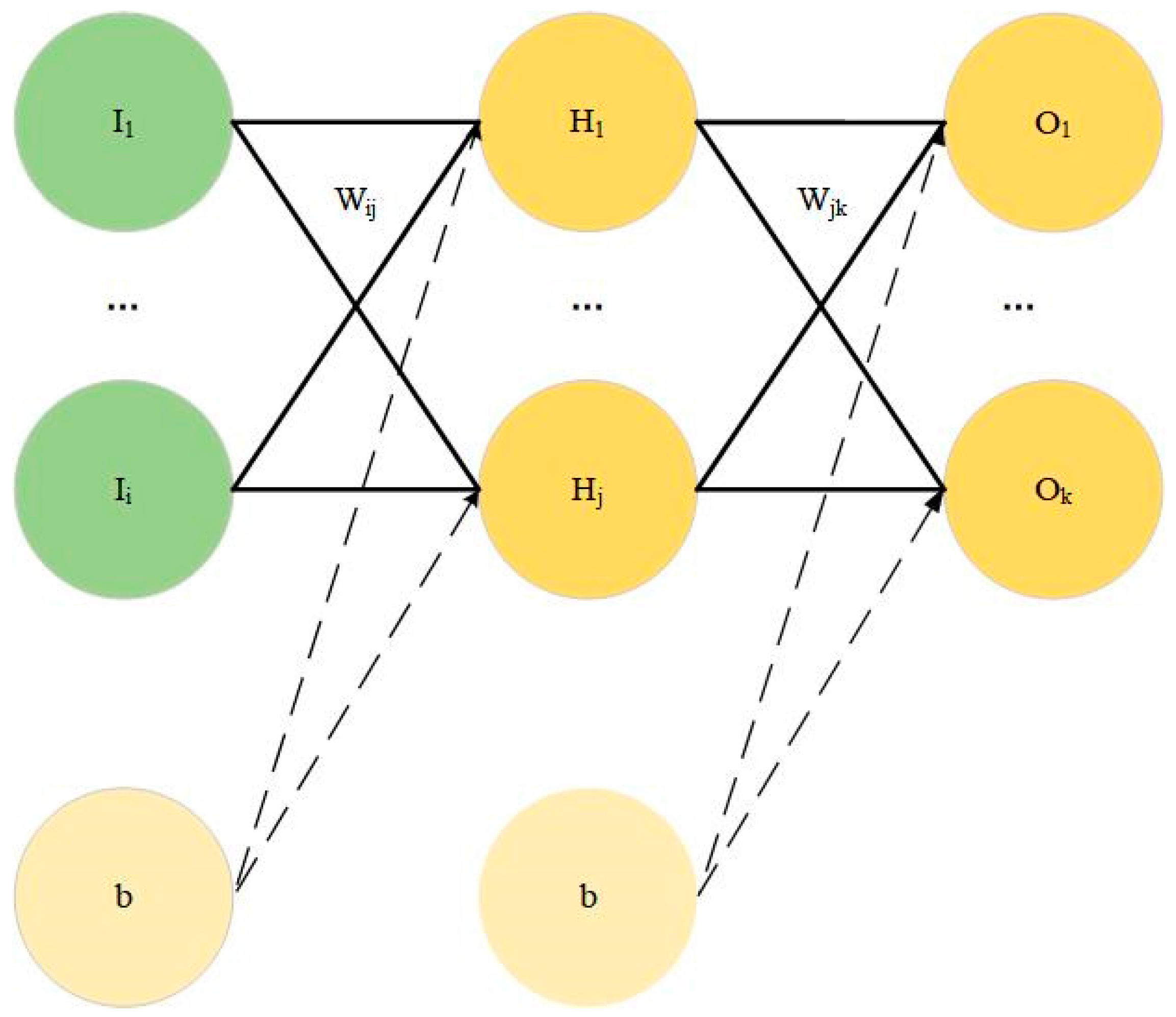
Figure 1. Schematic diagram of neural network method.
Remotesensing 13 00481 g001
Figure 2. Blue points represent the selected data (clear sky) from 00:30 to 01:30 on 1 February. Red points represent the abandoned data (cloud) from 00:30 to 01:30 on 1 February.
Remotesensing 13 00481 g002
Figure 3. The general framework of the ANN retrieval method (Met-ANN).
Remotesensing 13 00481 g003
Figure 4. The general framework of the improved 1D-Var retrieval method (Met-I1DVar).
Remotesensing 13 00481 g004
Figure 5. Covariance of temperature priori error.
Remotesensing 13 00481 g005
Figure 6. The RMSE between the simulated brightness temperature of each channel and the satellite observation brightness temperature, the blue line represents the long wave wavelengths and the red line represents the medium wave wavelengths.
Remotesensing 13 00481 g006
Figure 7. Select channels.
Remotesensing 13 00481 g007
Figure 8. Correction of observation data by ANN: the correlation coefficient of (a) training and (b) test.
Remotesensing 13 00481 g008
Figure 9. RMSE distribution of temperature on Met-I1DVar and 1D-Var.
Remotesensing 13 00481 g009
Figure 10. The general framework of our retrieval method (Met-Combine).
Remotesensing 13 00481 g010
Figure 11. (a) ME and (b) RMSE distribution of temperature on Met-ANN and Met-I1DVar.
Remotesensing 13 00481 g011
Figure 12. Red points represent the selected sounding data from 00:30 to 01:30 on 4 February. Blue points represent the selected observation data from 00:30 to 01:30 on 4 February.
Remotesensing 13 00481 g012
Figure 13. The box plot shows the MAE of the simulated brightness temperature and the observed brightness temperature (a,c,e,g,i) before and (b,d,f,h,j) after correction by the ANN method. The horizontal axis represents the wavenumber of the selected channels. The vertical axis represents MAE. The line in the middle of the box represents the median. The lines at the top and bottom of the box represent the upper and lower quartiles, respectively.
Remotesensing 13 00481 g013aRemotesensing 13 00481 g013b
Figure 14. Using the sounding data as the truth, (a) MAE and (b) RMSE distribution of temperature on Met-ANN and Met-I1DVar.
Remotesensing 13 00481 g014
Figure 15. Using the sounding data as the truth, (a) MAE and (b) RMSE distribution of temperature on Met-Combine and the product of GIIRS.
Remotesensing 13 00481 g015
Table 1. FY-4A/GIIRS instrument performance parameters.
ParametersIndicators
Spectral range (wavenumber)Long wave: 700–1130 cm−1
Medium wave: 1650–2250 cm−1
Spectral resolution0.625 cm−1
Number of channelsLong wave: 689
Medium wave: 961
SensitivityLong wave: 0.5–1.12 mW/(m2 sr cm−1)
Medium wave: 0.1–0.14 mW/(m2 sr cm−1)
Spatial resolution16 km (Nadir)
Time resolution<1 h (China regions)
<1/2 h (Meso-small scale)
Area of detection5000 × 5000 km2 (China regions)
1000 × 1000 km2 (Meso-small scale)
Spectral calibration accuracy10 ppm
Radiometric calibration accuracy1.5 K
Publisher’s Note: MDPI stays neutral with regard to jurisdictional claims in published maps and institutional affiliations.