
An Optical and SAR Based Fusion Approach for Mapping Surface Water Dynamics over Mainland China

 , , ,
, , ,
Abstract
1. Introduction
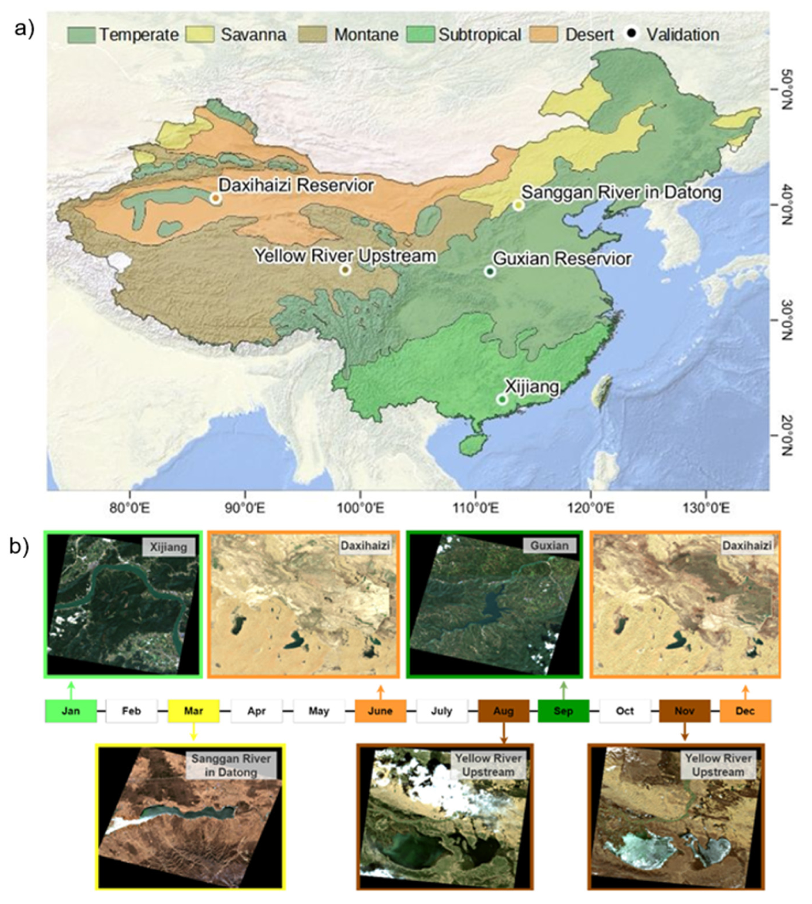
2. Study Area
3. Data and Methods
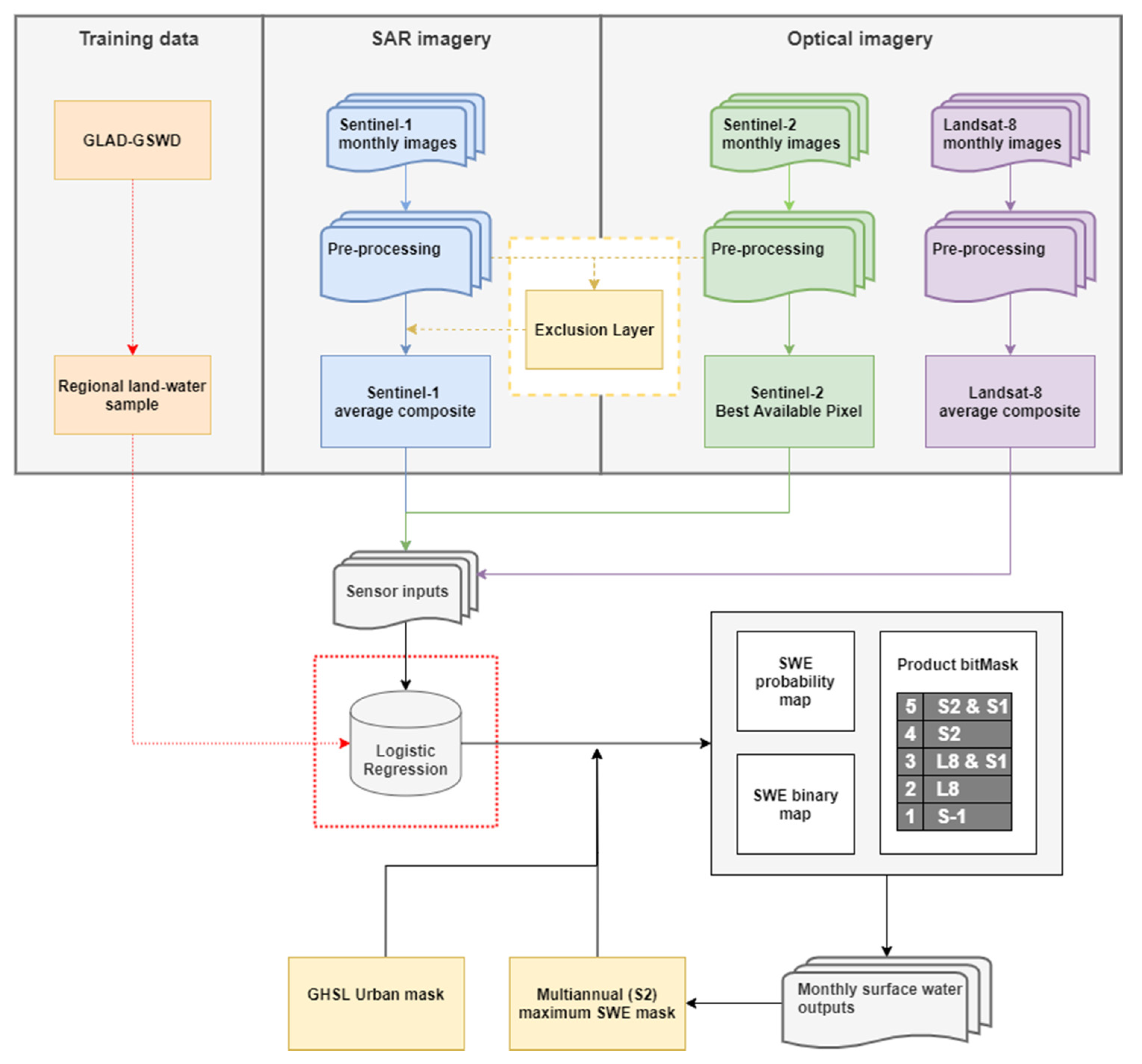
3.1. Background
3.2. Surface Water Mapping
3.2.1. Optical Data Processing
3.2.2. SAR Data Processing
3.2.3. Data Fusion
3.3. Validation
3.4. Product Intercomparison
4. Results
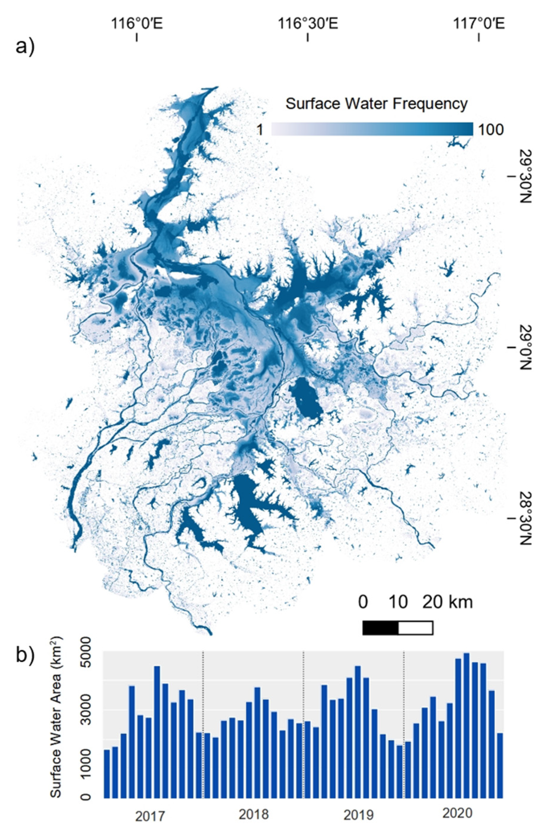
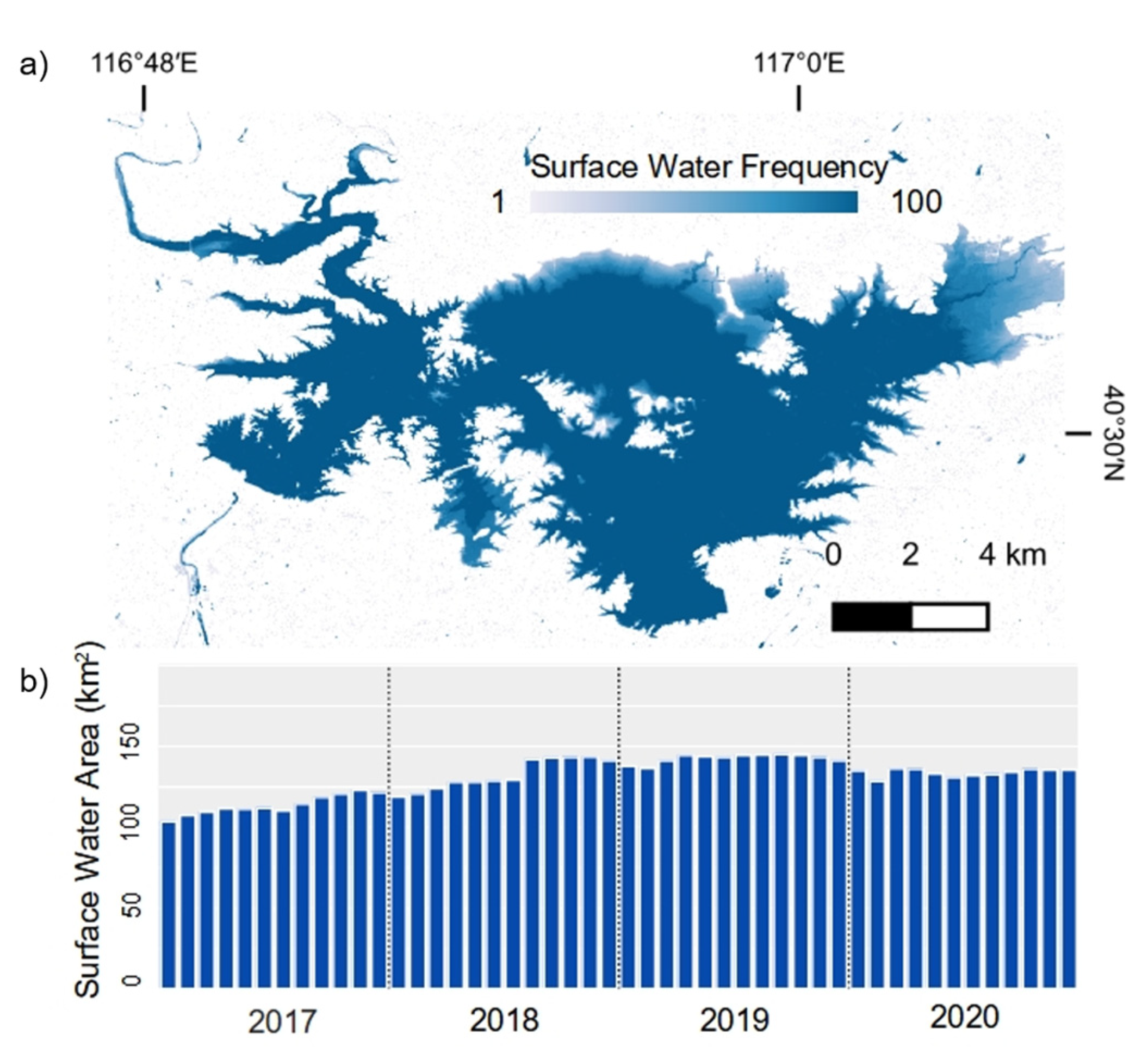
4.1. Water Occurrence Maps and Dynamics
4.2. Classification Accuracy
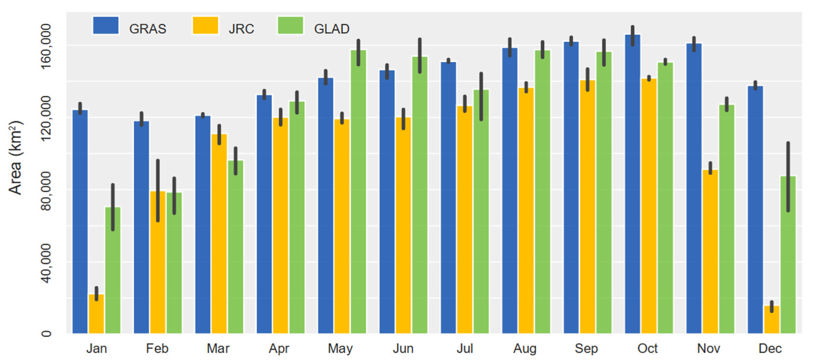
4.3. Area and Timeseries Comparisons with JRC-GSWE and GLAD GSWD
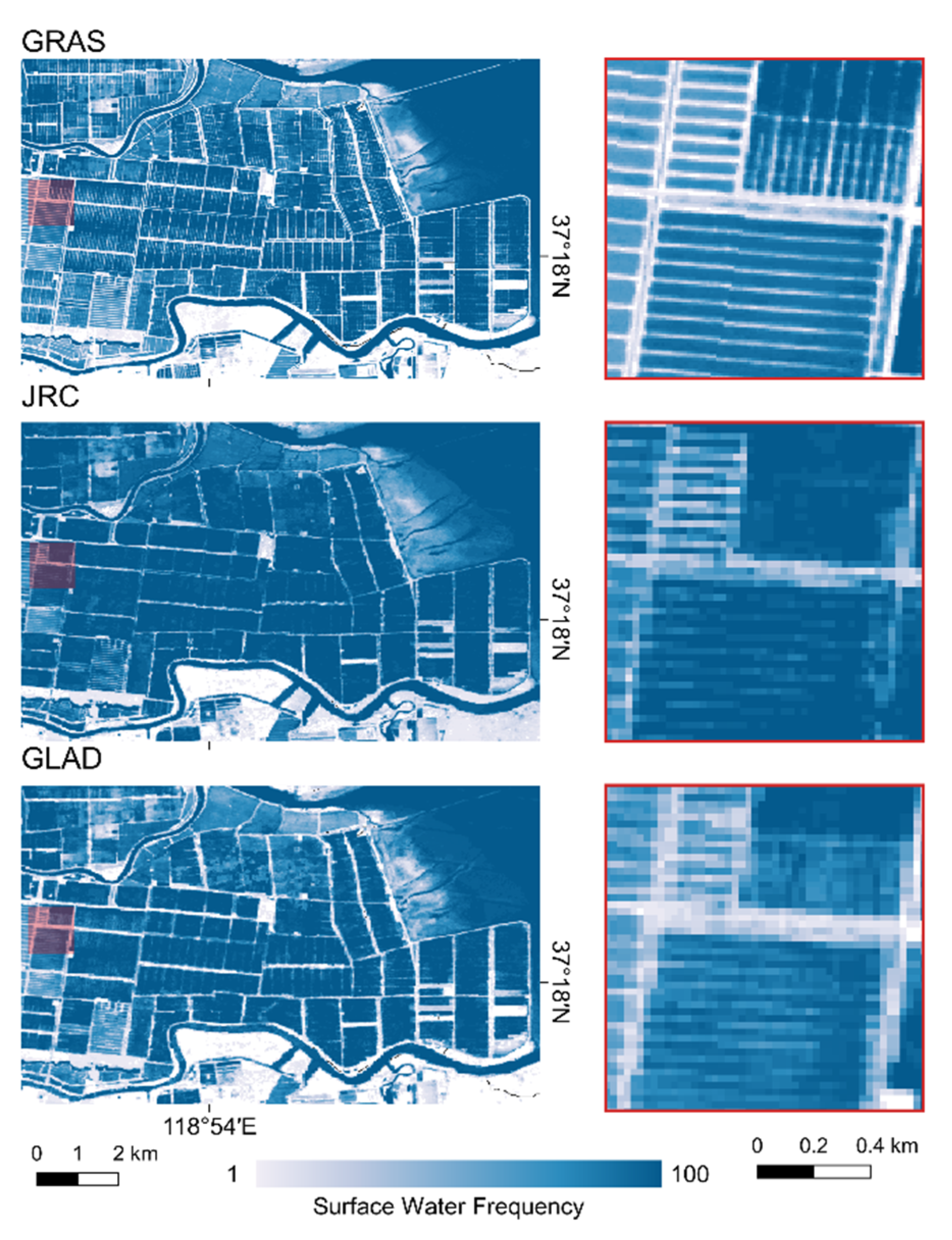
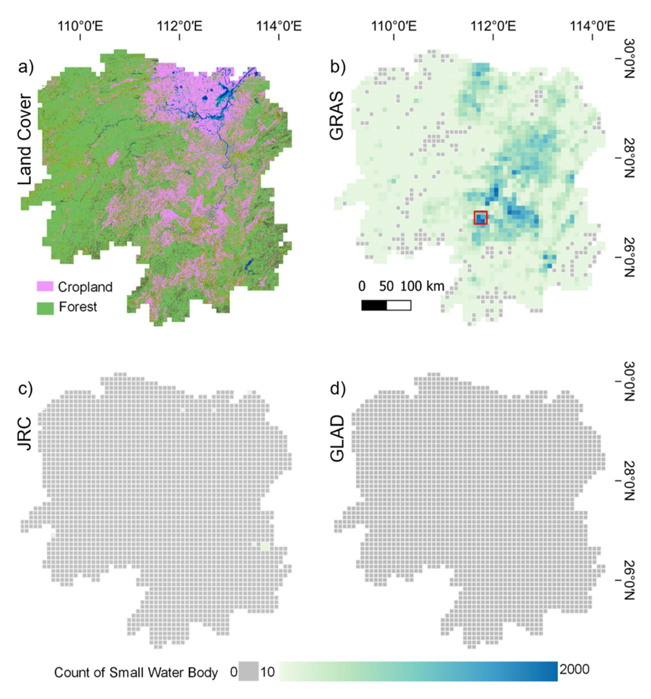
4.4. Visual Evaluation and Spatial Comparison with JRC-GSWE and GLAD-GSWD
5. Discussion
5.1. Accuracy
5.2. Temporal and Spatial Evaluation
5.3. Operational Water Monitoring
6. Conclusions
Author Contributions
Funding
Acknowledgments
Conflicts of Interest
References
- Smith, M.; Clausen, T.J. Revitalising IWRM for the 2030 Agenda; World Water Council Challenge Paper; World Water Council: London, UK, 2018. [Google Scholar]
- Hofste, R.W.; Reig, P.; Schleifer, L. 17 Countries, Home to One-Quarter of the World’s Population, Face Extremely High Water Stress. Available online: https://www.wri.org/blog/2019/08/17-countries-home-one-quarter-world-population-face-extremely-high-water-stress (accessed on 2 March 2021).
- Biggs, J.; von Fumetti, S.; Kelly-Quinn, M. The Importance of Small Waterbodies for Biodiversity and Ecosystem Services: Implications for Policy Makers. Hydrobiologia 2017, 793, 3–39. [Google Scholar] [CrossRef]
- Schumann, G.J.P.; Brakenridge, G.R.; Kettner, A.J.; Kashif, R.; Niebuhr, E. Assisting Flood Disaster Response with Earth Observation Data and Products: A Critical Assessment. Remote Sens. 2018, 10, 1230. [Google Scholar] [CrossRef]
- Melton, F.S.; Johnson, L.F.; Lund, C.P.; Pierce, L.L.; Michaelis, A.R.; Hiatt, S.H.; Guzman, A.; Adhikari, D.D.; Purdy, A.J.; Rosevelt, C.; et al. Satellite Irrigation Management Support With the Terrestrial Observation and Prediction System: A Framework for Integration of Satellite and Surface Observations to Support Improvements in Agricultural Water Resource Management. IEEE J. Sel. Top. Appl. Earth Obs. Remote Sens. 2012, 5, 1709–1721. [Google Scholar] [CrossRef]
- Midekisa, A.; Senay, G.; Henebry, G.M.; Semuniguse, P.; Wimberly, M.C. Remote Sensing-Based Time Series Models for Malaria Early Warning in the Highlands of Ethiopia. Malar. J. 2012, 11, 165. [Google Scholar] [CrossRef] [PubMed]
- Hardy, A.; Ettritch, G.; Cross, D.E.; Bunting, P.; Liywalii, F.; Sakala, J.; Silumesii, A.; Singini, D.; Smith, M.; Willis, T.; et al. Automatic Detection of Open and Vegetated Water Bodies Using Sentinel 1 to Map African Malaria Vector Mosquito Breeding Habitats. Remote Sens. 2019, 11, 593. [Google Scholar] [CrossRef]
- Cui, X.; Guo, X.; Wang, Y.; Wang, X.; Zhu, W.; Shi, J.; Lin, C.; Gao, X. Application of Remote Sensing to Water Environmental Processes under a Changing Climate. J. Hydrol. 2019, 574, 892–902. [Google Scholar] [CrossRef]
- Bastin, L.; Gorelick, N.; Saura, S.; Bertzky, B.; Dubois, G.; Fortin, M.J.; Pekel, J.F. Inland Surface Waters in Protected Areas Globally: Current Coverage and 30-Year Trends. PLoS ONE 2019, 14. [Google Scholar] [CrossRef]
- O’connor, B.; Moul, K.; Pollini, B.; De Lamo, X.; Simonson, W.; Allison, H.; Albrecht, F.; Guzinski, M.; Larsen, H.; Mcglade, J.; et al. EARTH OBSERVATION FOR SDG Compendium of Earth Observation contributions to the SDG Targets and Indicators. Available online: https://eo4society.esa.int/wp-content/uploads/2021/01/EO_Compendium-for-SDGs.pdf (accessed on 2 March 2021).
- Pekel, J.F.; Cottam, A.; Gorelick, N.; Belward, A.S. High-Resolution Mapping of Global Surface Water and Its Long-Term Changes. Nature 2016, 540, 418–422. [Google Scholar] [CrossRef]
- Pickens, A.H.; Hansen, M.C.; Hancher, M.; Stehman, S.V.; Tyukavina, A.; Potapov, P.; Marroquin, B.; Sherani, Z. Mapping and Sampling to Characterize Global Inland Water Dynamics from 1999 to 2018 with Full Landsat Time-Series. Remote Sens. Environ. 2020, 243. [Google Scholar] [CrossRef]
- Markham, B.L.; Helder, D.L. Forty-Year Calibrated Record of Earth-Reflected Radiance from Landsat: A Review. Remote Sens. Environ. 2012, 122, 30–40. [Google Scholar] [CrossRef]
- White, J.C.; Wulder, M.A. The Landsat Observation Record of Canada: 1972–2012. Can. J. Remote Sens. 2014, 39, 455–467. [Google Scholar] [CrossRef]
- Showstack, R. Sentinel Satellites Initiate New Era in Earth Observation. EOS 2014, 95, 239–240. [Google Scholar] [CrossRef]
- Ministry of Water Resources of the People’s Republic of China. Water Resources in China. Available online: http://www.mwr.gov.cn/english/mainsubjects/201604/P020160406508110938538.pdf (accessed on 23 April 2021).
- Jiang, Y. China’s Water Scarcity. J. Environ. Manage. 2009, 90, 3185–3196. [Google Scholar] [CrossRef]
- World Bank. Watershed: A New Era of Water Governance in China—Thematic Report; World Bank: Washington, DC, USA, 2019. [Google Scholar]
- Wang, Y.; Ma, J.; Xiao, X.; Wang, X.; Dai, S.; Zhao, B. Long-Term Dynamic of Poyang Lake Surface Water: A Mapping Work Based on the Google Earth Engine Cloud Platform. Remote Sens. 2019, 11, 313. [Google Scholar] [CrossRef]
- Xia, H.; Zhao, J.; Qin, Y.; Yang, J.; Cui, Y.; Song, H.; Ma, L.; Jin, N.; Meng, Q. Changes in Water Surface Area during 1989-2017 in the Huai River Basin Using Landsat Data and Google Earth Engine. Remote Sens. 2019, 11, 1824. [Google Scholar] [CrossRef]
- You, Q.; Chai, Y.; Jiang, C. Assessment of the Spatial Distribution of Surface Water Resources in Changchun, China Using Remote Sensing. J. Water Supply Res. Technol. AQUA 2018, 67, 490–497. [Google Scholar] [CrossRef]
- Yang, X.; Lu, X. Drastic Change in China’s Lakes and Reservoirs over the Past Decades. Sci. Rep. 2014, 4. [Google Scholar] [CrossRef] [PubMed]
- Jiang, W.; He, G.; Pang, Z.; Guo, H.; Long, T.; Ni, Y. Surface Water Map of China for 2015 (SWMC-2015) Derived from Landsat 8 Satellite Imagery. Remote Sens. Lett. 2020, 11, 265–273. [Google Scholar] [CrossRef]
- Feng, S.; Liu, S.; Huang, Z.; Jing, L.; Zhao, M.; Peng, X.; Yan, W.; Wu, Y.; Lv, Y.; Smith, A.R.; et al. Inland Water Bodies in China: Features Discovered in the Long-Term Satellite Data. Proc. Natl. Acad. Sci. USA 2019, 116, 25491–25496. [Google Scholar] [CrossRef]
- Jiang, L.; Nielsen, K.; Andersen, O.B.; Bauer-Gottwein, P. CryoSat-2 Radar Altimetry for Monitoring Freshwater Resources of China. Remote Sens. Environ. 2017, 200, 125–139. [Google Scholar] [CrossRef]
- Li, Y.; Niu, Z.; Xu, Z.; Yan, X. Construction of High Spatial-Temporal Water Body Dataset in China Based on Sentinel-1 Archives and GEE. Remote Sens. 2020, 12, 2413. [Google Scholar] [CrossRef]
- Feyisa, G.L.; Meilby, H.; Fensholt, R.; Proud, S.R. Automated Water Extraction Index: A New Technique for Surface Water Mapping Using Landsat Imagery. Remote Sens. Environ. 2014, 140, 23–35. [Google Scholar] [CrossRef]
- Acharya, T.D.; Subedi, A.; Lee, D.H. Evaluation of Water Indices for Surface Water Extraction in a Landsat 8 Scene of Nepal. Sensors 2018, 18, 2580. [Google Scholar] [CrossRef] [PubMed]
- Acharya, T.D.; Subedi, A.; Lee, D.H. Evaluation of Machine Learning Algorithms for Surface Water Extraction in a Landsat 8 Scene of Nepal. Sensors 2019, 19, 2769. [Google Scholar] [CrossRef] [PubMed]
- Du, Z.; Li, W.; Zhou, D.; Tian, L.; Ling, F.; Wang, H.; Gui, Y.; Sun, B. Analysis of Landsat-8 OLI Imagery for Land Surface Water Mapping. Remote Sens. Lett. 2014, 5, 672–681. [Google Scholar] [CrossRef]
- McFeeters, S.K. The Use of the Normalized Difference Water Index (NDWI) in the Delineation of Open Water Features. Int. J. Remote Sens. 1996, 17, 1425–1432. [Google Scholar] [CrossRef]
- Piao, S.; Ciais, P.; Huang, Y.; Shen, Z.; Peng, S.; Li, J.; Zhou, L.; Liu, H.; Ma, Y.; Ding, Y.; et al. The Impacts of Climate Change on Water Resources and Agriculture in China. Nature 2010, 467, 43–51. [Google Scholar] [CrossRef]
- Fan, X.; Liu, Y.; Wu, G.; Zhao, X. Compositing the Minimum NDVI for Daily Water Surface Mapping. Remote Sens. 2020, 12, 700. [Google Scholar] [CrossRef]
- Herndon, K.; Muench, R.; Cherrington, E.; Griffin, R. An Assessment of Surface Water Detection Methods for Water Resource Management in the Nigerien Sahel. Sensors 2020, 20, 431. [Google Scholar] [CrossRef]
- Glles, P.T. Remote Sensing and Cast Shadows in Mountainous Terrain. Photogramm. Eng. Remote Sens. 2001, 67, 833–839. [Google Scholar]
- Nobre, A.D.; Cuartas, L.A.; Hodnett, M.; Rennó, C.D.; Rodrigues, G.; Silveira, A.; Saleska, S. Height Above the Nearest Drainage–a Hydrologically Relevant New Terrain Model. J. Hydrol. 2011, 404, 13–29. [Google Scholar] [CrossRef]
- Twele, A.; Cao, W.; Plank, S.; Martinis, S. Sentinel-1-Based Flood Mapping: A Fully Automated Processing Chain. Int. J. Remote Sens. 2016, 37, 2990–3004. [Google Scholar] [CrossRef]
- Otsu, N. A Threshold Selection Method from Gray-Level Histograms. IEEE Trans. Syst. Man. Cybern. 1979, 9, 62–66. [Google Scholar] [CrossRef]
- Donchyts, G.; Baart, F.; Winsemius, H.; Gorelick, N.; Kwadijk, J.; van de Giesen, N. Earth’s Surface Water Change over the Past 30 Years. Nat. Clim. Chang. 2016, 6, 810–813. [Google Scholar] [CrossRef]
- Khandelwal, A.; Karpatne, A.; Marlier, M.E.; Kim, J.; Lettenmaier, D.P.; Kumar, V. An Approach for Global Monitoring of Surface Water Extent Variations in Reservoirs Using MODIS Data. Remote Sens. Environ. 2017, 202, 113–128. [Google Scholar] [CrossRef]
- Millard, K.; Brown, N.; Stiff, D.; Pietroniro, A. Automated Surface Water Detection from Space: A Canada-Wide, Open-Source, Automated, near-Real Time Solution. Can. Water Resour. J. Rev. Can. Ressour. Hydr. 2020, 45, 304–323. [Google Scholar] [CrossRef]
- Wieland, M.; Martinis, S. Large-Scale Surface Water Change Observed by Sentinel-2 during the 2018 Drought in Germany. Int. J. Remote Sens. 2020, 41, 4742–4756. [Google Scholar] [CrossRef]
- Bangira, T.; Alfieri, S.M.; Menenti, M.; van Niekerk, A. Comparing Thresholding with Machine Learning Classifiers for Mapping Complex Water. Remote Sens. 2019, 11, 1351. [Google Scholar] [CrossRef]
- Man, C.D.; Nguyen, T.T.; Bui, H.Q.; Lasko, K.; Nguyen, T.N.T. Improvement of Land-Cover Classification over Frequently Cloud-Covered Areas Using Landsat 8 Time-Series Composites and an Ensemble of Supervised Classifiers. Int. J. Remote Sens. 2018, 39, 1243–1255. [Google Scholar] [CrossRef]
- Schneider, R.; Godiksen, P.N.; Villadsen, H.; Madsen, H.; Bauer-Gottwein, P. Application of CryoSat-2 Altimetry Data for River Analysis and Modelling. Hydrol. Earth Syst. Sci. 2017, 21, 751–764. [Google Scholar] [CrossRef]
- Clement, M.A.; Kilsby, C.G.; Moore, P. Multi-Temporal Synthetic Aperture Radar Flood Mapping Using Change Detection. J. Flood Risk Manag. 2018, 11, 152–168. [Google Scholar] [CrossRef]
- Greifeneder, F.; Wagner, W.; Sabel, D.; Naeimi, V. Suitability of SAR Imagery for Automatic Flood Mapping in the Lower Mekong Basin. Int. J. Remote Sens. 2014, 35, 2857–2874. [Google Scholar] [CrossRef]
- Hostache, R.; Matgen, P.; Wagner, W. Change Detection Approaches for Flood Extent Mapping: How to Select the Most Adequate Reference Image from Online Archives? Int. J. Appl. Earth Obs. Geoinf. 2012, 19, 205–213. [Google Scholar] [CrossRef]
- Schlaffer, S.; Matgen, P.; Hollaus, M.; Wagner, W. Flood Detection from Multi-Temporal SAR Data Using Harmonic Analysis and Change Detection. Int. J. Appl. Earth Obs. Geoinf. 2015, 38, 15–24. [Google Scholar] [CrossRef]
- Hu, S.; Qin, J.; Ren, J.; Zhao, H.; Ren, J.; Hong, H. Automatic Extraction of Water Inundation Areas Using Sentinel-1 Data for Large Plain Areas. Remote Sens. 2020, 12, 243. [Google Scholar] [CrossRef]
- Ovakoglou, G.; Cherif, I.; Alexandridis, T.K.; Pantazi, X.-E.; Tamouridou, A.-A.; Moshou, D.; Tseni, X.; Raptis, I.; Kalaitzopoulou, S.; Mourelatos, S. Automatic Detection of Surface-Water Bodies from Sentinel-1 Images for Effective Mosquito Larvae Control. J. Appl. Remote Sens. 2021, 15, 1–23. [Google Scholar] [CrossRef]
- Huang, W.; DeVries, B.; Huang, C.; Lang, M.W.; Jones, J.W.; Creed, I.F.; Carroll, M.L. Automated Extraction of Surface Water Extent from Sentinel-1 Data. Remote Sens. 2018, 10, 797. [Google Scholar] [CrossRef]
- Manjusree, P.; Prasanna Kumar, L.; Bhatt, C.M.; Rao, G.S.; Bhanumurthy, V. Optimization of Threshold Ranges for Rapid Flood Inundation Mapping by Evaluating Backscatter Profiles of High Incidence Angle SAR Images. Int. J. Disaster Risk Sci. 2012, 3, 113–122. [Google Scholar] [CrossRef]
- O’Grady, D.; Leblanc, M.; Gillieson, D. Relationship of Local Incidence Angle with Satellite Radar Backscatter for Different Surface Conditions. Int. J. Appl. Earth Obs. Geoinf. 2013, 24, 42–53. [Google Scholar] [CrossRef]
- Martinis, S.; Plank, S.; Ćwik, K. The Use of Sentinel-1 Time-Series Data to Improve Flood Monitoring in Arid Areas. Remote Sens. 2018, 10, 583. [Google Scholar] [CrossRef]
- Bioresita, F.; Puissant, A.; Stumpf, A.; Malet, J.-P. A Method for Automatic and Rapid Mapping of Water Surfaces from Sentinel-1 Imagery. Remote Sens. 2018, 10, 217. [Google Scholar] [CrossRef]
- Hahmann, T.; Martinis, S.; Twele, A.; Roth, A.; Buchroithner, M. Extraction of Water and Flood Areas from SAR Data. In Proceedings of the 7th European Conference on Synthetic Aperture Radar, Friedrichshafen, Germany, 2–5 June 2008; pp. 1–4. [Google Scholar]
- Song, Y.-S.; Sohn, H.-G.; Park, C.-H. Efficient Water Area Classification Using Radarsat-1 SAR Imagery in a High Relief Mountainous Environment. Photogramm. Eng. Remote Sens. 2007, 73, 285–296. [Google Scholar] [CrossRef]
- Joshi, N.; Baumann, M.; Ehammer, A.; Fensholt, R.; Grogan, K.; Hostert, P.; Jepsen, M.R.; Kuemmerle, T.; Meyfroidt, P.; Mitchard, E.T.A.; et al. A Review of the Application of Optical and Radar Remote Sensing Data Fusion to Land Use Mapping and Monitoring. Remote Sens. 2016, 8, 70. [Google Scholar] [CrossRef]
- Bioresita, F.; Puissant, A.; Stumpf, A.; Malet, J.-P.P. Fusion of Sentinel-1 and Sentinel-2 Image Time Series for Permanent and Temporary Surface Water Mapping. Int. J. Remote Sens. 2019, 40. [Google Scholar] [CrossRef]
- Markert, K.N.; Chishtie, F.; Anderson, E.R.; Saah, D.; Griffin, R.E. On the Merging of Optical and SAR Satellite Imagery for Surface Water Mapping Applications. Results Phys. 2018, 9, 275–277. [Google Scholar] [CrossRef]
- van Leeuwen, B.; Tobak, Z.; Kovács, F. Sentinel-1 and-2 Based near Real Time Inland Excess Water Mapping for Optimized Water Management. Sustainability 2020, 12, 2854. [Google Scholar] [CrossRef]
- Gorelick, N.; Hancher, M.; Dixon, M.; Ilyushchenko, S.; Thau, D.; Moore, R. Google Earth Engine: Planetary-Scale Geospatial Analysis for Everyone. Remote Sens. Environ. 2017, 202, 18–27. [Google Scholar] [CrossRef]
- Main-Knorn, M.; Pflug, B.; Louis, J.; Debaecker, V.; Müller-Wilm, U.; Gascon, F. Sen2Cor for Sentinel-2. In Image and Signal Processing for Remote Sensing XXIII; Bruzzone, L., Bovolo, F., Benediktsson, J.A., Eds.; SPIE: Bellingham, DC, USA, 2017; p. 3. [Google Scholar]
- Hollstein, A.; Segl, K.; Guanter, L.; Brell, M.; Enesco, M. Ready-to-Use Methods for the Detection of Clouds, Cirrus, Snow, Shadow, Water and Clear Sky Pixels in Sentinel-2 MSI Images. Remote Sens. 2016, 8, 666. [Google Scholar] [CrossRef]
- Zhu, Z.; Wang, S.; Woodcock, C.E. Improvement and Expansion of the Fmask Algorithm: Cloud, Cloud Shadow, and Snow Detection for Landsats 4–7, 8, and Sentinel 2 Images. Remote Sens. Environ. 2015, 159, 269–277. [Google Scholar] [CrossRef]
- Foga, S.; Scaramuzza, P.L.; Guo, S.; Zhu, Z.; Dilley Jr, R.D.; Beckmann, T.; Schmidt, G.L.; Dwyer, J.L.; Hughes, M.J.; Laue, B. Cloud Detection Algorithm Comparison and Validation for Operational Landsat Data Products. Remote Sens. Environ. 2017, 194, 379–390. [Google Scholar] [CrossRef]
- Airbus. Copernicus DEM Product Handbook. Available online: https://spacedata.copernicus.eu/documents/20126/0/GEO1988-CopernicusDEM-SPE-002_ProductHandbook_I1.00+%281%29.pdf/40b2739a-38d3-2b9f-fe35-1184ccd17694?t=1612269439996 (accessed on 2 March 2021).
- Google. Sentinel-1 Algorithms. Available online: https://developers.google.com/earth-engine/guides/sentinel1 (accessed on 12 April 2021).
- Dinerstein, E.; Olson, D.; Joshi, A.; Vynne, C.; Burgess, N.D.; Wikramanayake, E.; Hahn, N.; Palminteri, S.; Hedao, P.; Noss, R. An Ecoregion-Based Approach to Protecting Half the Terrestrial Realm. Bioscience 2017, 67, 534–545. [Google Scholar] [CrossRef]
- Pesaresi, M.; Ehrlich, D.; Ferri, S.; Florczyk, A.; Freire, S.; Halkia, M.; Julea, A.; Kemper, T.; Soille, P.; Syrris, V. Operating Procedure for the Production of the Global Human Settlement Layer from Landsat Data of the Epochs 1975, 1990, 2000 and 2014; JRC Technical Report; European Commission, Joint Research Centre, Institute for the Protection and Security of the Citizen: Ispra, Italy, 2016. [Google Scholar]
- Niva, V.; Cai, J.; Taka, M.; Kummu, M.; Varis, O. China’s Sustainable Water-Energy-Food Nexus by 2030: Impacts of Urbanization on Sectoral Water Demand. J. Clean. Prod. 2020, 251, 119755. [Google Scholar] [CrossRef]
- Li, Y.; Zhong, Y.; Shao, R.; Yan, C.; Jin, J.; Shan, J.; Li, F.; Ji, W.; Bin, L.; Zhang, X. Modified Hydrological Regime from the Three Gorges Dam Increases the Risk of Food Shortages for Wintering Waterbirds in Poyang Lake. Glob. Ecol. Conserv. 2020, 24, e01286. [Google Scholar] [CrossRef]
- Reliefweb. Thousands Battle Floods along Yangtze River. Available online: https://reliefweb.int/report/china/china-thousands-battle-floods-along-yangtze-river (accessed on 2 March 2021).
- Reliefweb. Yangtze River Sees First Flood This Year. Available online: https://reliefweb.int/report/china/yangtze-river-sees-first-flood-year (accessed on 2 March 2021).
- Reliefweb. China Battles Unprecedented Floods around Its Largest Freshwater Lake. Available online: https://reliefweb.int/report/china/china-battles-unprecedented-floods-around-its-largest-freshwater-lake (accessed on 2 March 2021).
- Li, J.; Wang, C.; Xu, L.; Wu, F.; Zhang, H.; Zhang, B. Multitemporal Water Extraction of Dongting Lake and Poyang Lake Based on an Automatic Water Extraction and Dynamic Monitoring Framework. Remote Sens. 2021, 13, 865. [Google Scholar] [CrossRef]
- Peisert, C.; Sternfeld, E. Quenching Beijing’s Thirst: The Need for Integrated Management for the Endangered Miyun Reservoir. China Environ. Ser. 2005, 7, 33–45. [Google Scholar]
- Qiu, J.; Shen, Z.; Huang, M.; Zhang, X. Exploring Effective Best Management Practices in the Miyun Reservoir Watershed, China. Ecol. Eng. 2018, 123, 30–42. [Google Scholar] [CrossRef]
- Lai, Y.; Zhang, J.; Song, Y.; Cao, Y. Comparative Analysis of Different Methods for Extracting Water Body Area of Miyun Reservoir and Driving Forces for Nearly 40 Years. J. Indian Soc. Remote Sens. 2020, 48, 451–463. [Google Scholar] [CrossRef]
- Xinhuanet. Beijing’s largest reservoir supplies water to dried-up river. Available online: http://www.xinhuanet.com/english/2019-06/01/c_138108168.htm (accessed on 2 March 2021).
- Downing, J.A.; Prairie, Y.T.; Cole, J.J.; Duarte, C.M.; Tranvik, L.J.; Striegl, R.G.; McDowell, W.H.; Kortelainen, P.; Caraco, N.F.; Melack, J.M. The Global Abundance and Size Distribution of Lakes, Ponds, and Impoundments. Limnol. Oceanogr. 2006, 51, 2388–2397. [Google Scholar] [CrossRef]
- Buchhorn, M.; Lesiv, M.; Tsendbazar, N.-E.; Herold, M.; Bertels, L.; Smets, B. Copernicus Global Land Cover Layers—Collection 2. Remote Sens. 2020, 12, 1044. [Google Scholar] [CrossRef]
- Farr, T.G.; Rosen, P.A.; Caro, E.; Crippen, R.; Duren, R.; Hensley, S.; Kobrick, M.; Paller, M.; Rodriguez, E.; Roth, L. The Shuttle Radar Topography Mission. Rev. Geophys. 2007, 45. [Google Scholar] [CrossRef]
- Yamazaki, D.; Ikeshima, D.; Tawatari, R.; Yamaguchi, T.; O’Loughlin, F.; Neal, J.C.; Sampson, C.C.; Kanae, S.; Bates, P.D. A High-accuracy Map of Global Terrain Elevations. Geophys. Res. Lett. 2017, 44, 5844–5853. [Google Scholar] [CrossRef]
- Martinis, S.; Kuenzer, C.; Wendleder, A.; Huth, J.; Twele, A.; Roth, A.; Dech, S. Comparing Four Operational SAR-Based Water and Flood Detection Approaches. Int. J. Remote Sens. 2015, 36, 3519–3543. [Google Scholar] [CrossRef]
- Zeng, L.; Schmitt, M.; Li, L.; Zhu, X.X. Analysing Changes of the Poyang Lake Water Area Using Sentinel-1 Synthetic Aperture Radar Imagery. Int. J. Remote Sens. 2017, 38, 7041–7069. [Google Scholar] [CrossRef]
- Mason, D.C.; Speck, R.; Devereux, B.; Schumann, G.J.-P.; Neal, J.C.; Bates, P.D. Flood Detection in Urban Areas Using TerraSAR-X. IEEE Trans. Geosci. Remote Sens. 2009, 48, 882–894. [Google Scholar] [CrossRef]
- Wang, Y.; Li, Z.; Zeng, C.; Xia, G.-S.; Shen, H. An Urban Water Extraction Method Combining Deep Learning and Google Earth Engine. IEEE J. Sel. Top. Appl. Earth Obs. Remote Sens. 2020, 13, 768–781. [Google Scholar] [CrossRef]
- Liu, J.; Jiang, L.; Zhang, X.; Druce, D.; Kittel, C.M.M.; Tøttrup, C.; Bauer-Gottwein, P. Impacts of Water Resources Management on Land Water Storage in the North China Plain: Insight from Multi-Mission Earth Observations. J. Hydrol. 2021. [Google Scholar] [CrossRef]
- Gao, H.; Birkett, C.; Lettenmaier, D.P. Global Monitoring of Large Reservoir Storage from Satellite Remote Sensing. Water Resour. Res. 2012, 48. [Google Scholar] [CrossRef]
- Downing, J.A. Emerging Global Role of Small Lakes and Ponds: Little Things Mean a Lot. Limnetica 2008, 29, 9–24. [Google Scholar]
- Chen, W.; He, B.; Nover, D.; Lu, H.; Liu, J.; Sun, W.; Chen, W. Farm Ponds in Southern China: Challenges and Solutions for Conserving a Neglected Wetland Ecosystem. Sci. Total Environ. 2019, 659, 1322–1334. [Google Scholar] [CrossRef] [PubMed]
- Lei, Y.; Yao, T.; Yang, K.; Sheng, Y.; Kleinherenbrink, M.; Yi, S.; Bird, B.W.; Zhang, X.; Zhu, L.; Zhang, G. Lake Seasonality across the Tibetan Plateau and Their Varying Relationship with Regional Mass Changes and Local Hydrology. Geophys. Res. Lett. 2017, 44, 892–900. [Google Scholar] [CrossRef]
- UN-Water. Indicator 6.6.1 Change in the Extent of Water-Related Ecosystems over Time. Available online: https://www.sdg6monitoring.org/indicator-661/ (accessed on 23 April 2021).


| Sample Locations | Validation Date | Gaofen Sensor | Ice | OA | Land UA | Land PA | Water UA | Water PA |
|---|---|---|---|---|---|---|---|---|
| Guxian | 22-09-2019 | GF-1 | no | 99% | 99% | 99% | 98% | 97% |
| Yellow River Upstream | 13-11-2019 | GF-6 | yes | 90% | 88% | 89% | 91% | 90% |
| Yellow River Upstream | 10-08-2019 | GF-1 | no | 93% | 90% | 93% | 95% | 92% |
| Xijiang | 27-01-2019 | GF-1 | no | 93% | 93% | 95% | 94% | 91% |
| Daxihaizi | 20-12-2019 | GF-1 | no | 95% | 96% | 98% | 88% | 79% |
| Daxihaizi | 14-06-2019 | GF-2 | no | 98% | 98% | 99% | 93% | 85% |
| Sanggan | 18-03-2019 | GF-6 | yes | 97% | 99% | 97% | 95% | 97% |
| Land | Water | Samples | ||||||
|---|---|---|---|---|---|---|---|---|
| OA | UA | PA | UA | PA | Water | Land | Total | |
| Seasonal Strata | 87% | 88% | 90% | 86% | 83% | 1785 | 2568 | 4353 |
| All data | 94% | 94% | 97% | 94% | 89% | 5082 | 8631 | 13713 |
Publisher’s Note: MDPI stays neutral with regard to jurisdictional claims in published maps and institutional affiliations. |
© 2021 by the authors. Licensee MDPI, Basel, Switzerland. This article is an open access article distributed under the terms and conditions of the Creative Commons Attribution (CC BY) license (https://creativecommons.org/licenses/by/4.0/).
Share and Cite
Druce, D.; Tong, X.; Lei, X.; Guo, T.; Kittel, C.M.M.; Grogan, K.; Tottrup, C. An Optical and SAR Based Fusion Approach for Mapping Surface Water Dynamics over Mainland China. Remote Sens. 2021, 13, 1663. https://doi.org/10.3390/rs13091663
Druce D, Tong X, Lei X, Guo T, Kittel CMM, Grogan K, Tottrup C. An Optical and SAR Based Fusion Approach for Mapping Surface Water Dynamics over Mainland China. Remote Sensing. 2021; 13(9):1663. https://doi.org/10.3390/rs13091663
Chicago/Turabian StyleDruce, Daniel, Xiaoye Tong, Xia Lei, Tao Guo, Cecile M.M. Kittel, Kenneth Grogan, and Christian Tottrup. 2021. "An Optical and SAR Based Fusion Approach for Mapping Surface Water Dynamics over Mainland China" Remote Sensing 13, no. 9: 1663. https://doi.org/10.3390/rs13091663
APA StyleDruce, D., Tong, X., Lei, X., Guo, T., Kittel, C. M. M., Grogan, K., & Tottrup, C. (2021). An Optical and SAR Based Fusion Approach for Mapping Surface Water Dynamics over Mainland China. Remote Sensing, 13(9), 1663. https://doi.org/10.3390/rs13091663