Abstract
Traditional applications of Interferometric Synthetic Aperture Radar (InSAR) data involved inverting an interferogram stack to determine the average displacement velocity. While this approach has useful applications in continuously deforming regions, much information is lost by simply fitting a line through the time series. Thanks to regular acquisitions across most of the the world by the ESA Sentinel-1 satellite constellation, we are now in a position to explore opportunities for near-real time deformation monitoring. In this paper we present a statistical approach for detecting offsets and gradient changes in InSAR time series. Our key assumption is that 5 years of Sentinel-1 data is sufficient to calculate the population standard deviation of the detection variables. Our offset detector identifies statistically significant peaks in the first, second and third difference series. The gradient change detector identifies statistically significant movements in the second derivative series. We exploit the high spatial resolution of Sentinel-1 data and the spatial continuity of geophysical deformation signals to filter out false positive detections that arise due to signal noise. When combined with near-real time processing of InSAR data these detectors, particularly the gradient change, could be used to detect incipient ground deformation associated with geophysical phenomena, for example from landslides or volcanic eruptions.
1. Introduction
Interferometric Synthetic Aperture Radar (InSAR) is now an established technique for monitoring ground deformation [1]. Repeat data collection from satellite missions has enabled the combination of multiple sets of interferograms, in various network approaches, to create time series of ground displacements (see review by Minh et al. [2]). While some researchers are beginning to interrogate the variations in line-of-sight displacement time series (e.g., [3,4,5,6,7,8,9]), most simply plot a best-fit through the time series to get the average line-of-sight displacement rate. This approach undermines the true strength of InSAR time series analysis, particularly in the context of missions such as Sentinel-1 that are committed to providing consistent data for the next few decades at a greater temporal resolution than previous SAR missions. While the average deformation rate is a useful measure for some applications, to determine linear subsidence rates for example [10,11], much information is lost by simply fitting a line through the time series, which makes identifying abrupt changes more difficult. Indeed, depending on the underlying processes, ground deformation is rarely linear in time. For example, volcanoes may remain dormant for many years before a sudden or gradual onset of ground deformation preceding an eruption, or ground subsidence may continue slowly at the same rate for many years before suddenly accelerating. Each of these produce distinct deformation patterns that can be detected in InSAR time series.
The consistency in data collection by the Sentinel-1 satellite constellation and its short revisit time (12 day repeats for most of the world and 6 day repeats over Europe), provides an opportunity to develop a near-real time early warning system that can monitor and detect changes in ground motion and provide alerts to responsible authorities that changes are occurring at their site of interest. For example, at volcanoes where 1 in 3 active volcanoes now have InSAR measurements [12], or at a mining site where incipient motion could be a precursor to tailings collapse [13]. In this paper, we describe a new methodology that exploits the existing archive and continuous data collection from the Sentinel-1 satellite to detect anomalous ground motions statistically.
Time series change detection is not new. There are many existing methods from Bayesian change point detection, CUMSUM, segmentation and machine learning methods (see Aminikhanghahi and Cook [14] for a review). These are used extensively in the technology sector, e.g., by streaming services to monitor spikes in complaints, and by analysts to monitor changes in stock markets [15,16]. These methods are designed to accurately detect changes in a single, albeit long, time series. Most of these methods are not suitable for InSAR time series where in any one scene we may have hundreds of thousands if not millions of pixels, each with its own deformation history. The computational costs of applying complex methods to InSAR time series is therefore prohibitive.
There are generally two approaches for automatic time series change detection, offline methods and online methods. Offline methods determine changes in an existing series, where data exists before and after a change point. This is relatively easier and prone to fewer detection errors. These methods have already been applied to InSAR to determine change points. For example Berti et al. [17] used the Bayesian Information Criterion (BIC) to determine break points considering the whole time series for a given pixel. However, for near-real time analysis we require online detection methods where only information preceding a data point can be used to check for changes. This enables continuous monitoring as new data are added to the time series.
Recently, machine learning approaches have been used to search through large volumes of InSAR images to detect patterns that may be related to geological hazards [18,19,20]. These methods generally require large volumes of training data and have mostly been applied to detect volcanic deformation in radar interferograms or InSAR time series [8,21].
Our method, detailed in this paper, uses a hybrid offline-online statistical approach that is parallelised and vectorised for computational efficiency in order to deal with the large data volumes associated with InSAR time series. Therefore it is not constrained to detecting deformation from any specific geophysical process. Additionally, we exploit the spatial correlation of deformation signals to reduce the false positives in our detections.
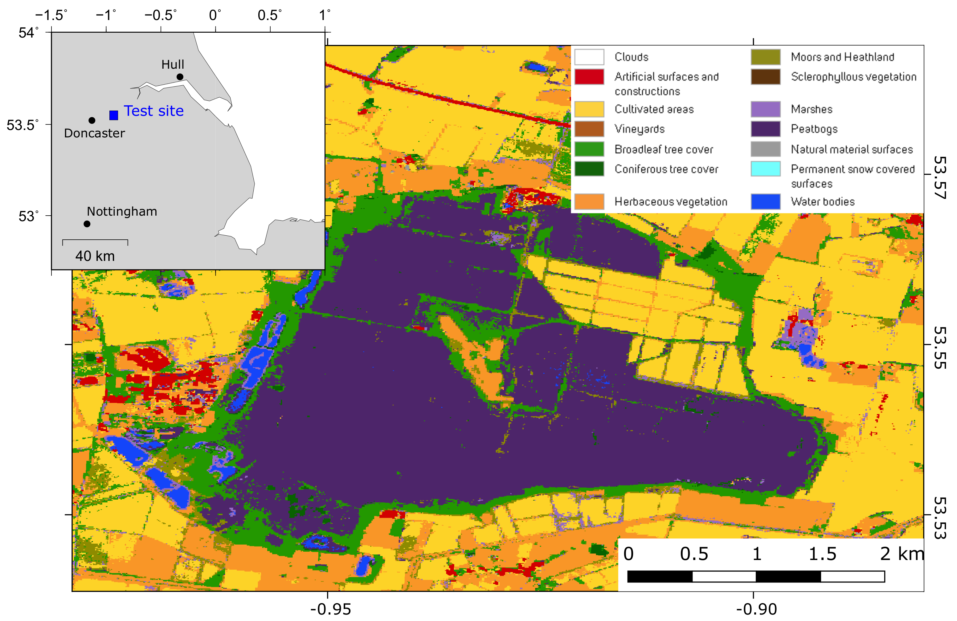
We apply and test our method to an InSAR time series dataset generated over Hatfield Moors (Yorkshire, UK) (Figure 1). Hatfield Moors along with Thorne, Goole and Crowle Moors make up the Humberhead Peatlands, the largest raised bog wilderness in lowland Britain covering a total of 2887 hectares [22,23]. This remnant of a large wetland is a Natural England nature reserve that overlies a former hydrocarbon reservoir where gas was extracted between 1986 to the late 1990s. Since 2000, this site has been used as a gas storage facility run by Scottish Power [24]. Natural Gas is compressed and pumped into the natural underground sandstone reservoir for storage and then extracted when needed. 4.1 billion cubic tonnes of gas can be stored here. As part of the SENSE project [25], the British Geological Survey is monitoring the ground stability conditions at this site as an analogue for Carbon Capture and Storage (CCS) sites. It is hoped that monitoring potential ground motion related to the injection and extraction of stored gas will allow the development of InSAR based techniques to monitor on-land CCS sites in the future.

Figure 1.
Location of the Hatfield Moors test site. The main figure is the land cover classification for the area using Sentinel-2 satellite imagery [22], which shows the study site is mostly peatbog surrounded by agricultural fields. The south and western edges of the site are bounded by lakes and ponds.
2. Methods
2.1. InSAR Processing and Time Series Analysis
We downloaded 257 Sentinel-1 single look complex (SLC) images from descending track 81 acquired between January 2015 and May 2020 over the Hatfield Moors test site in the UK (Longitude, latitude: −1.01, 53.58), and performed initial InSAR processing by forming interferograms with every 2 consecutive pairs of images using the Interferometric synthetic aperture radar Scientific Computing Environment (ISCE) software [26,27]. To improve the signal-to-noise ratio we multilooked each image by 9 pixels in range and 3 pixels in azimuth giving pixel sizes of approximately 50 m.
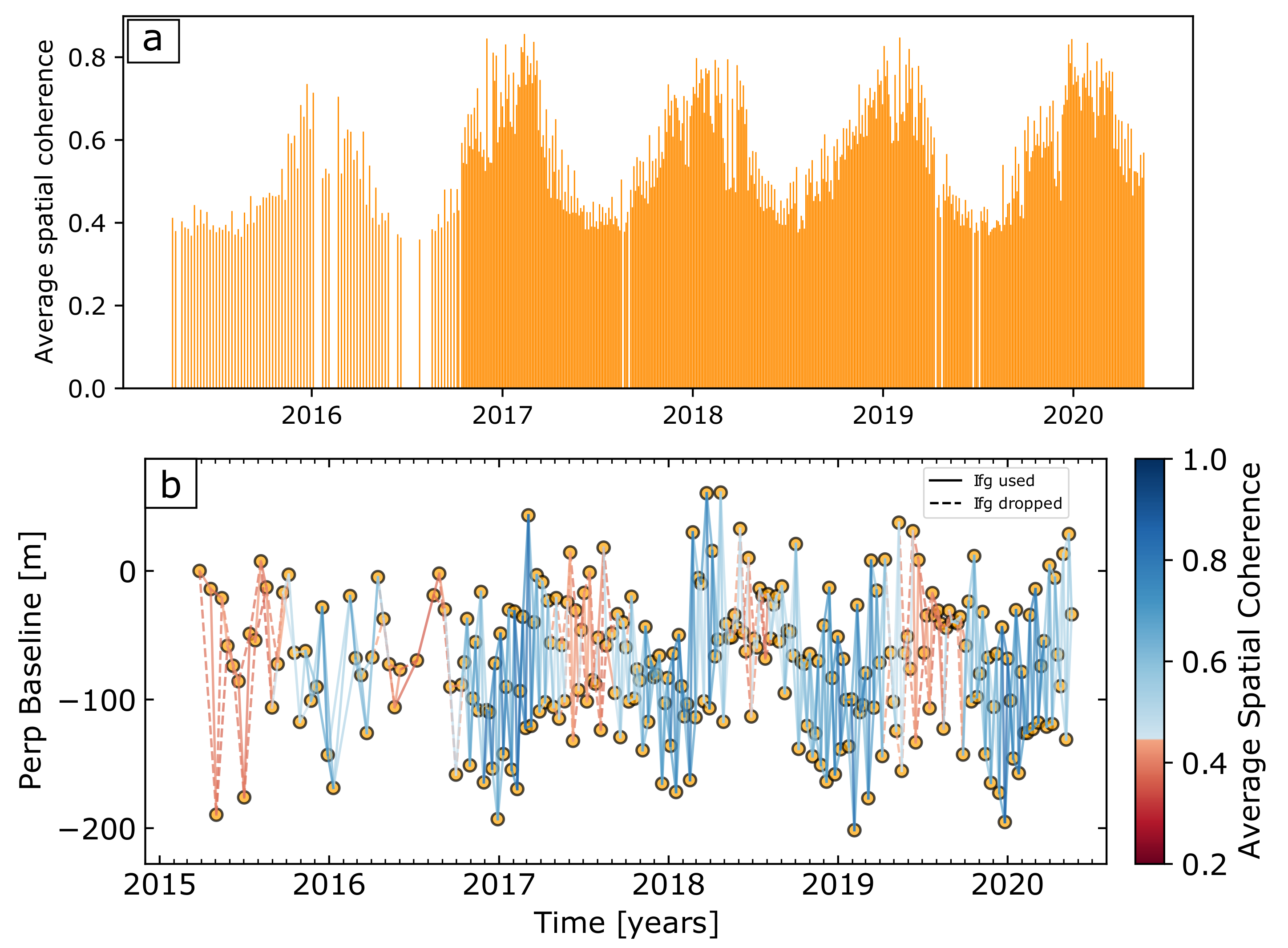
We processed the resulting 509 small baseline interferogram stack using the Miami INsar Time-series software in PYthon (MintPy) [28,29] to produce a geocoded line-of-sight displacement time series for every pixel in the dataset. The average spatial coherence history of the interferograms shows a clear annual signal with generally poor coherence during the summer months (Figure 2). This is probably due to decorrelation from atmospheric signals, surface water in the peat and actively growing vegetation, which incoherently scatters the radar waves. We therefore removed interferograms with an average coherence less than 0.45, unless it was required to maintain network connectivity, which resulted in the removal of 85 interferograms. We applied corrections for atmospheric noise using ERA5 reanalysis weather model data according to the method of Jolivet et al. [30], and used the SRTM 30m digital elevation model [31] to estimate the topographic error. Additionally we remove a ramp from each interferogram to remove any remaining long wavelength trends. Mintpy does not apply any spatial filters but uses snaphu connected components as a guide for the time series inversion [28,32]. We estimate and correct unwrapping errors in the interferograms using the bridging and phase closure method functionality in MintPy [28].

Figure 2.
(a) The average spatial coherence of all initial interferograms represented as a bar centred on the middle of the primary and secondary acquisition dates. The coherence history shows a clear annual cyclicity between a maximum of about 0.8 and a minimum of about 0.4. (b) Baseline-time plot for the interferograms formed in this study. Each line represents an interferogram, colour coded with the average spatial coherence of that image. The dashed red lines are interferograms with average coherence below the threshold value of 0.45 and so were discarded unless they were needed to maintain network connectivity (solid red lines).
2.2. Changes in Displacement Time Series
For most geophysical applications there are two types of changes in deformation time series that are of interest: offsets and changes in displacement gradients. Note that our aim is to detect displacement changes in both scenarios, and so regions moving at a constant displacement rate are not of interest for this study unless there is a change from steady-state.
In the sections below we describe the two components of the algorithm that detect each of these changes.
2.2.1. Offset Detection
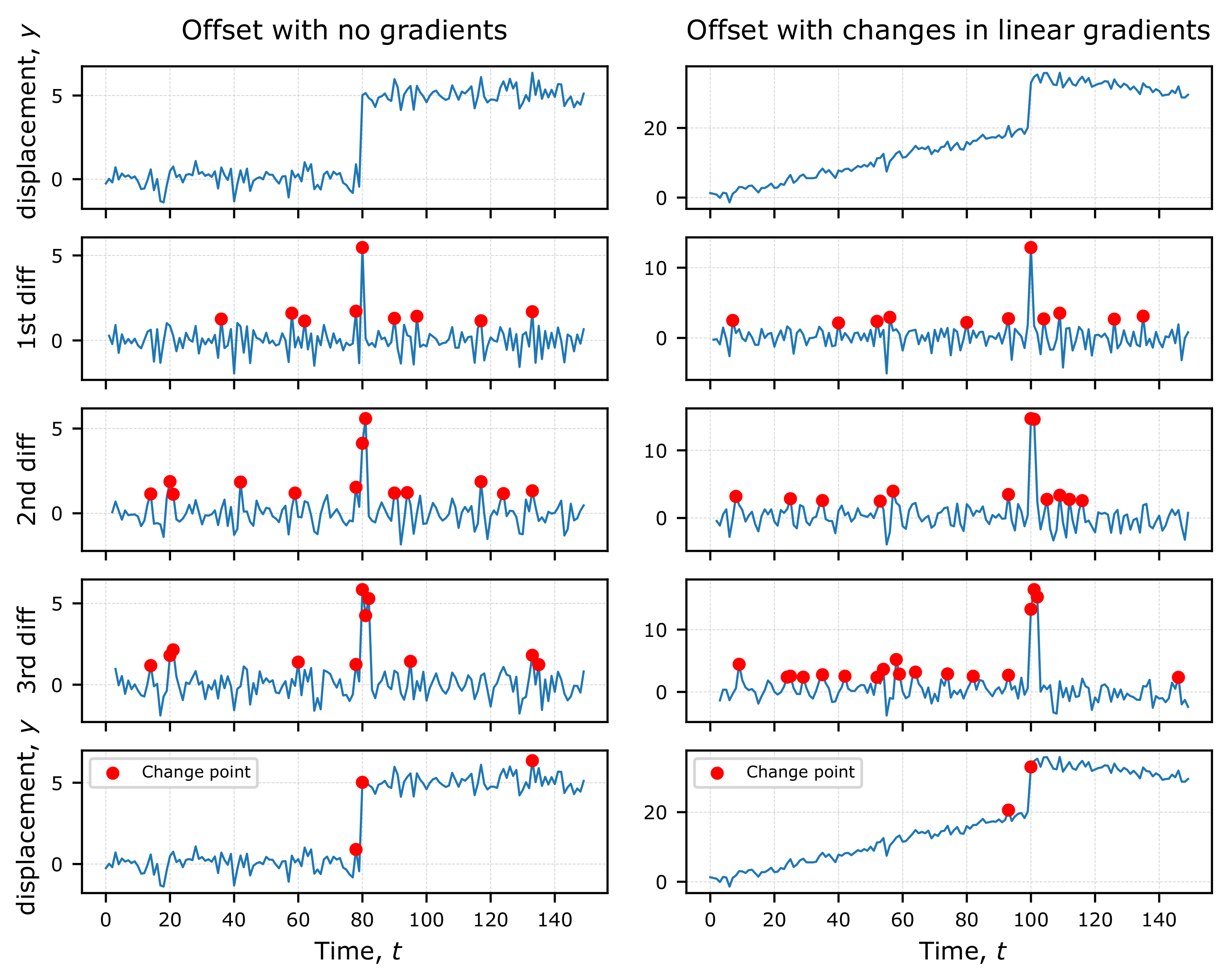
Offsets in time series take the form of an instantaneous jump (Figure 3). In order to detect these jumps we look for peaks in the displacement difference time series. For the difference series of order d:
where is the displacement at acquisition date t and k is the lag step size. B is the backshift operator [33]:
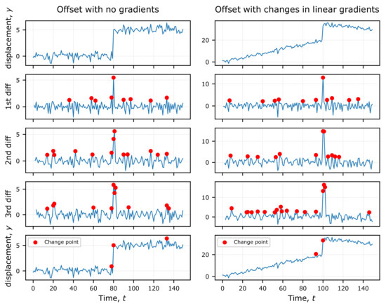
Figure 3.
Two synthetic offset change examples. The top row are displacement time series with offsets at and respectively. There are no gradients before and after the offset in the first example, and different gradients before and after the offset in the second example. There are numerous change detections (shown in red circles) for each of the difference series. But these are reduced when we take the intersection of the 1st, 2nd and 3rd difference detections (bottom row).
In the case of the first difference, the change between consecutive observations in the original series, and so that the first difference series is:
While the original displacement time series may not be stationary due to the presence of linear trends and or seasonality, our assumption is that the first, second and third difference time series are stationary [33], meaning that they will have no predictable patterns in the long-term. We test this assumption using an Augmented Dickey-Fuller (ADF) test [34] on each difference time series, which as the null hypothesis states that a unit root is present in the series, the principle cause behind non-stationarity. If the p-value from the ADF test is less than 5% we reject the null hypothesis, meaning the time series is stationary.
In our tests we find that in all cases the first difference series is stationary. However, in cases of extreme seasonality the second and third difference series are not stationary. Differences with longer temporal separations are more likely to be affected by any strong gradients in the times series (e.g., seasonality), meaning they are less likely to be stationary. In such cases we take the second order difference, i.e. the difference of the difference with in Equation (1), which results in stationarity (Figure 4). This is a routine procedure in time series analysis [33,35].
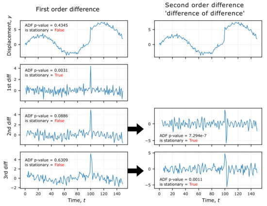
Figure 4.
Stationarity tests on the first and second order difference series. The top row is a synthetic time series with strong seasonal displacements and an offset at . We test for stationarity using the Augmented Dickey-Fuller (ADF) test and reject the null hypothesis (the series is not stationary) if the ADF p-value is less than 0.05. We show that the synthetic displacement series is not stationary but the first difference is. The second and third difference fail the stationarity test so we calculate the second order ‘difference of difference’ series for these, after which they pass the stationarity test.
While gradients, or changes that occur slowly over multiple time steps, are removed when differencing, offsets are retained in the difference series because they are an instantaneous jump in displacement. Offsets in the displacement time series manifest as a peak in the difference series. The challenge now becomes a question of how to statistically distinguish these peaks from the noise level. To do this we first need to characterise the noise level in the difference series using only 90% of the data (between the 5% and 95% quantiles), assuming that the remaining points may contain offsets that will bias the standard deviation calculation:
where is the subset of N observations of the difference series that lie between the 5% and 95% quantiles, and is the standard deviation of the difference series. For the online detector our assumption is that the standard deviation remains the same for all new observations added to the time series.
Assuming the noise in the displacement time series is i.i.d. Gaussian, the detection problem now becomes a matter of calculating the Student’s t-statistic and testing for statistical significance at a given threshold, here set to 0.95. Since we want to perform an online test with new incoming data points we use the form of the test statistic for unequal sample sizes but similar variance [36].
We perform a test with each new point one at a time, . And so the equation reduces to:
is the mean of the difference series, which we assume remains constant. Since differencing removes all trends from the displacement time series and assuming noise in the displacement series is Gaussian and drifts in the series are small, then is small compared to the noise in the data. Computationally this is now much more efficient because the denominator is also a constant, making the calculation a vectorised operation on . Points that pass the significance test at the 95% confidence level are labelled as candidate change points in the time series.
In order to increase our confidence and reduce false positives in the detections, we perform this step on the first, second and third difference time series ( respectively), and take the intersection of points detected by all three series independently as the confirmed offset change point (Figure 3).
2.2.2. Gradient Change Detection
In this case we are interested in detecting changes in the local displacement gradient within a given temporal window. Therefore we aim to detect peaks in the second derivative of the series in local windows. To improve the signal-to-noise ratio of the derivative calculations we first filter each time series with a rolling mean function over a small window [37], which should be a fraction of the gradient window size. The gradient window can be specified depending on the types of potential changes of interest, but must cover at least 2 data points in time (in order to be able to calculate a gradient). Ideally the window will cover at least 5 measurement points in time to get a more accurate measurement of the local gradient.
where is the second derivative series determined by calculating the local second derivative of the displacement time series in rolling windows of size (in days), with the result of the calculation in each window placed in the centre. In practice this involves first determining the slope of all displacement measurements within moving windows of size to get the first derivative series. And then repeating this step with the same window size to get the second derivative series. The choice of window size will determine the types of gradient changes that can be detected. Larger windows will be able to detect gradient changes that occur over a longer time period. Smaller windows are more sensitive to noise in the time series.
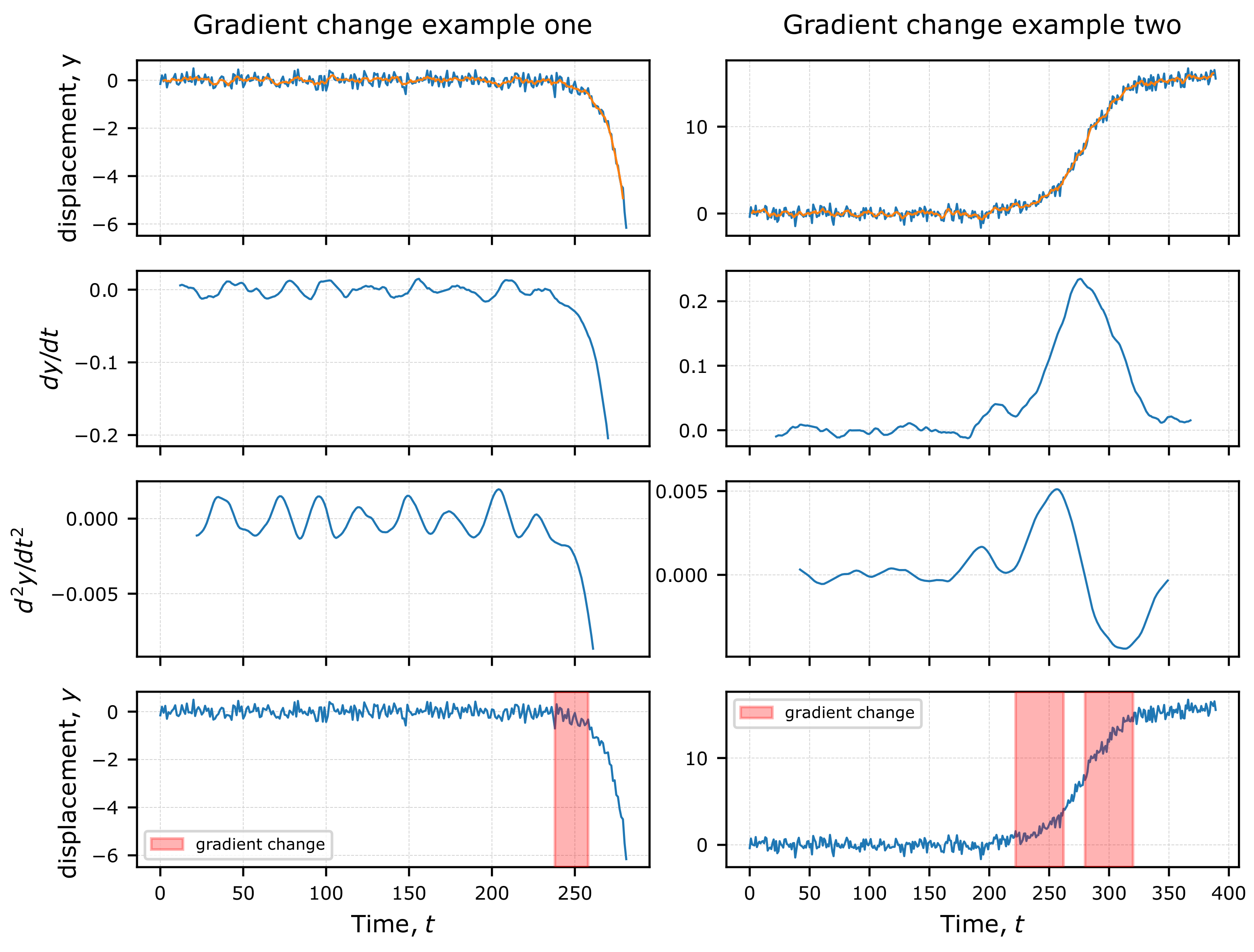
We perform the same standard deviation estimation and Student’s t-test described in the offset change detection above but in this case we only do the hypothesis test once on the second derivative time series. Unlike the offset detections, the gradient change points represent windows of size within which a change in gradient has occurred (Figure 5).
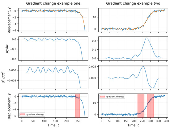
Figure 5.
Two synthetic gradient change examples. The orange line in the top figure is the 15-day smoothed series. Example one uses a detection window of 20 days while we use 40 days for example two.
2.2.3. Spatial Filtering
A unique strength and challenge of InSAR time series analysis is that not only do we have a relatively dense sampling in time, we also have a dense pixel sampling in space. At full resolution (∼5 m in range and ∼15 m in azimuth) a 250 km by 200 km Sentinel-1 radar scene may contain on the order of tens to hundreds of millions of pixels, each with its own time series that can be treated independently in terms of the change detection method described above.
Such large quantities of data presents a challenge in terms of efficient data processing. But it is also an opportunity. Most geophysical signals of interest have a spatial pattern across multiple pixels. For example, volcanic inflation signal or vertical displacement due to subsurface fluid injection/extraction may occur over several kilometres, which could encompass several thousand to tens of thousands of pixels. Even smaller signals from active landslides will generally include several tens or hundreds of pixels.
If a change point is detected at time t at pixel , then there is a strong likelihood that if the deformation is real then it will be detected at neighbouring pixels too. If there is no such change point at neighbouring pixels then it is likely that the detected change is a false positive.
Therefore, to reduce the occurrence of false positives in the detections we apply a 2-dimensional Gaussian filter to each time step in our time series. Practically this involves the convolution of a Gaussian kernel of size of and with each binary detection image (0 for no detection and 1 for detection) at every time step. After smoothing, detection pixels with a value less than 0.5 are discarded. The result of this filtering is the reduction of spatially isolated detections, which we assume are false positives.
3. Results
We apply and test our method on an InSAR stack processed over Hatfield Moors in the UK (Figure 1). Since 2000 Scottish Power have been using the natural underground sandstone reservoir beneath the site as a gas storage facility. The superficial land cover of the site consists mostly of peatland surrounded by agricultural fields. The south and western edges of the site are bounded by lakes and ponds.
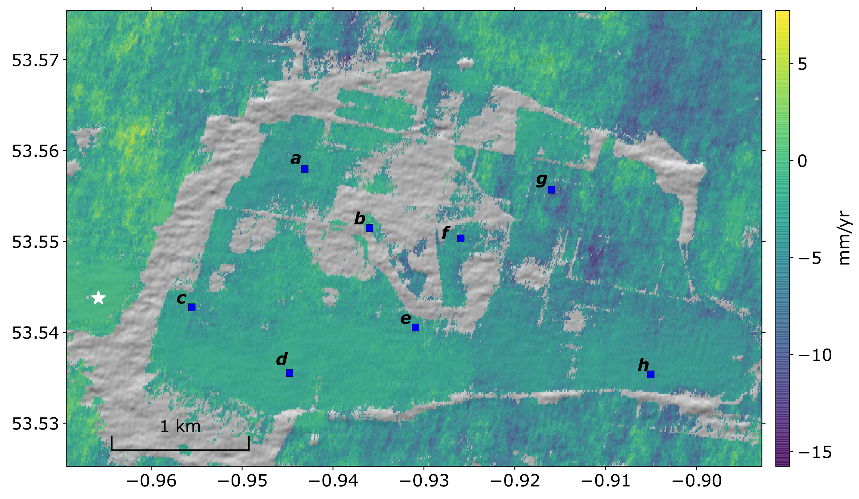
Of the 509 Sentinel-1 interferograms processed over the Hatfield Moors test site, we discarded 85 due to poor coherence (Figure 2b). We inverted the remaining 424 interferograms to form a displacement time series over the region spanning 257 dates between 28 March 2015 and 18 May 2020. The average line-of-sight velocity through the time series is shown in (Figure 6), where negative blue colours represent increase in line-of-sight displacement rate from the satellite. While most pixels have an average velocity between mm/yr, there are a few pixels to the east with range increase up to 15 mm/yr.
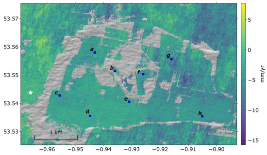
Figure 6.
The average line-of-sight velocity for the study region. The white star at (lon lat: −0.966, 53.544) is the reference pixel. Blue colours represent distance increase from the satellite. Clear areas indicate where no measurements were possible due to poor coherence. The blue squares are the locations of the pixel time series shown in Figure 7. Points a, c, d, e and h correspond to the Peatbogs land cover class in Figure 1, point b is on Herbaceous vegetation and point g on Cultivated area.
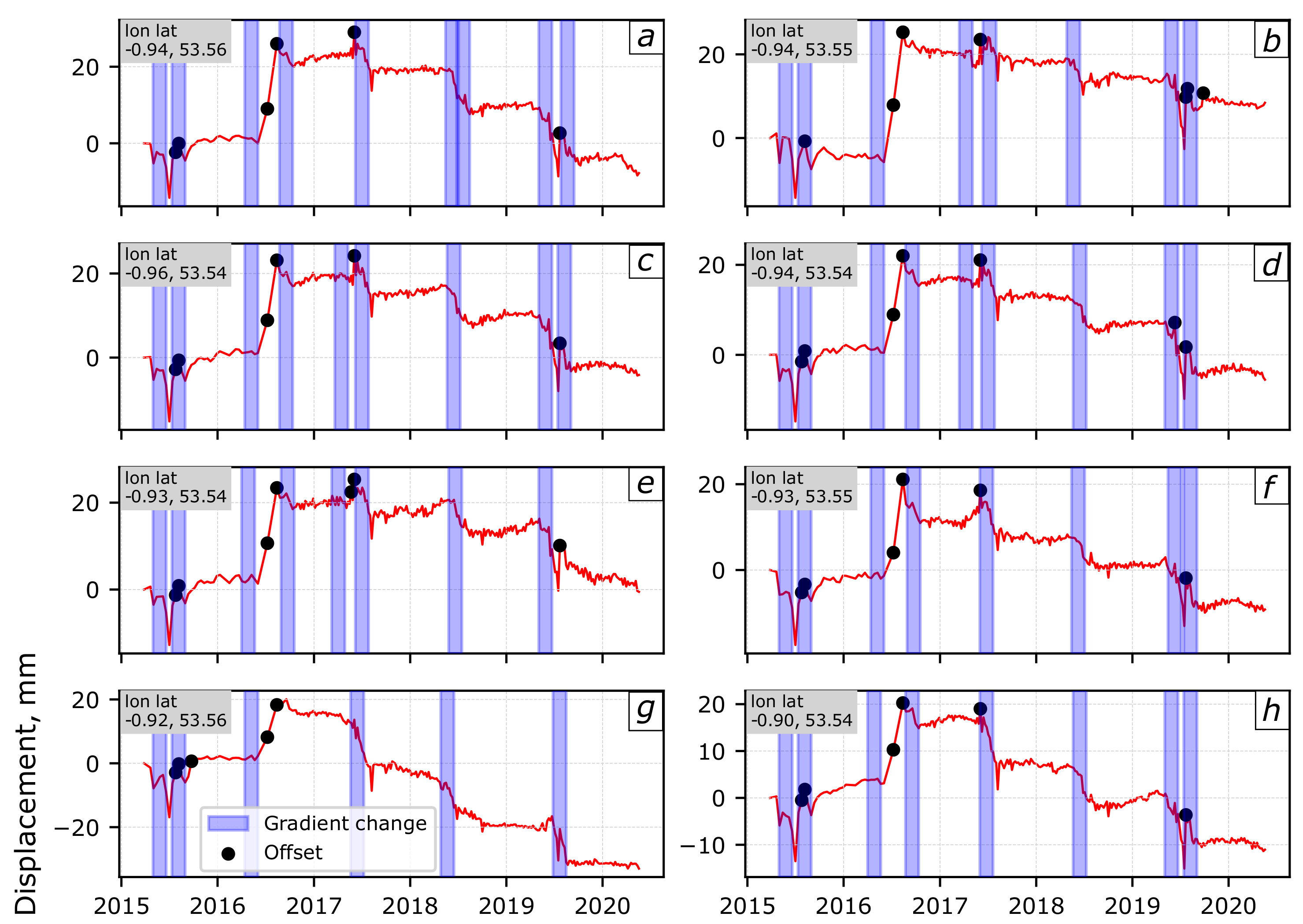
We apply our change detection algorithm to determine offsets and gradient changes for each of the pixel time series in this image. For the gradient change detection we chose an arbitrary window size of 50 days and a smoothing window of 15 days. A random selection of the results covering the study area are shown in Figure 7, where the black circles are detected offsets and blue bars represent the window in which we detect a gradient change. Due to the small region of study, the time series show similar deformation patterns. In general, upon visual inspection we are able to pick out the main turning points within each series, particularly the steps in displacement.
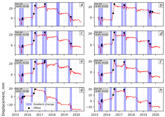
Figure 7.
Selected pixel time series covering the study region with offset and gradient changes detected using our algorithm. The location of each pixel is indicated in Figure 6. We chose a window size of 50 days for the gradient change detection. With our detection method we are able to pick out most of the turning points within each time series.
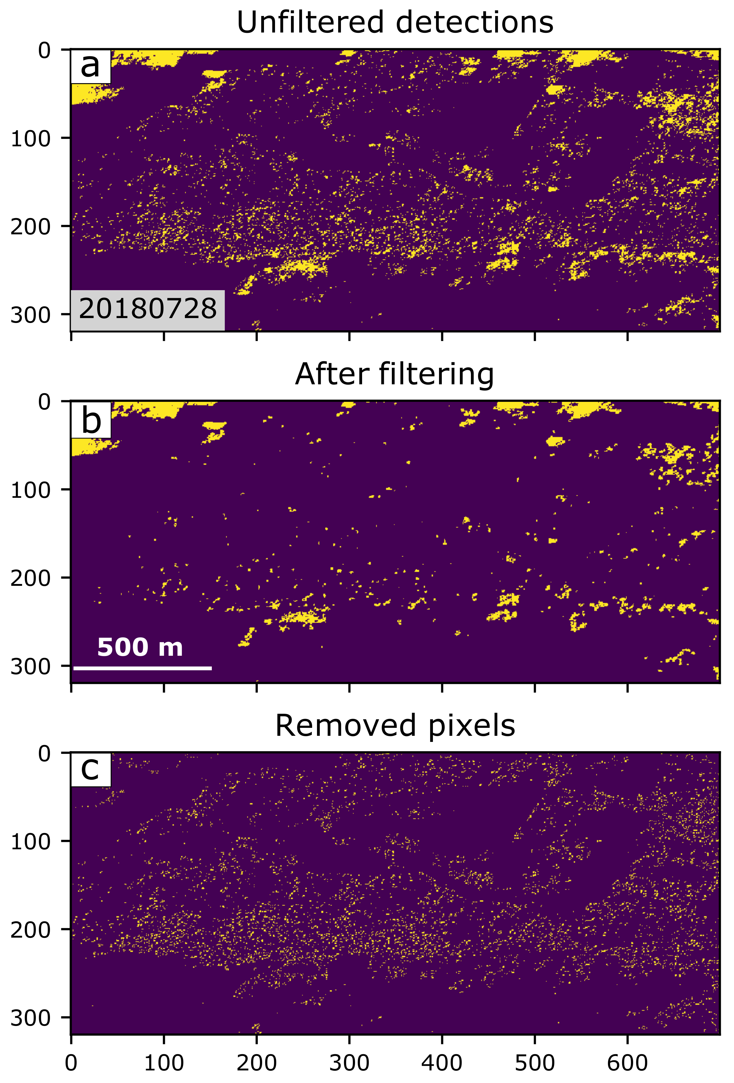
We remove isolated pixel detections, which we assume are false positives, using the method described in Section 2.2.3. We apply the Gaussain blur filter to each 2D detection map in the time series using a kernel window of approximately 200 m. On average, spatial filtering resulted in a 26% reduction in the number of detections across the entire stack (Figure 8).
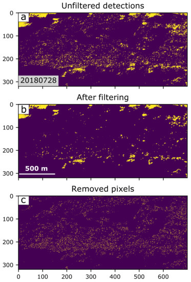
Figure 8.
An example of how the Gaussian blur filter is able to remove isolated pixel detections, which we assume are false positives, leaving the spatially continuous detection clusters. Yellow points are pixels that our algorithm has highlighted as having a change from steady-state (offset or gradient) at this time (28 July 2018). Purple colours are either NaN pixels or pixels with no changes in their displacements. (a) Shows the raw detections using our algorithm, and (b) the results after spatial filtering. (c) are the spatially isolated pixels that were removed by the filter. Axis represent the rows and columns of the pixels
While the aim of this paper is not to interpret the physical cause behind these patterns, we suspect that the steps in the time series are related to a combination of groundwater level changes within the peat, which is known to follow annual precipitation (e.g., [38,39]), and periodic gas injection and withdrawal from the sediments in this region. Disentangling these signals will require further investigation and field studies. These are ongoing as part of the SENSE research project (https://sense-act.eu, accessed on 27 January 2021).
4. Discussion
Previous InSAR time series detectors relied on machine learning methods to train an algorithm on specific changes in a time series resulting from ground deformation, for example volcano inflation (e.g., [8,18,21,40]). The method described in this paper is purely statistical and therefore process independent, meaning that changes are detected in the time series regardless of the geophysical cause behind it. While our approach is more broadly applicable, it does mean that we are more prone to false positives due to signal noise, but we show that we are able to reduce these by spatial filtering.
Currently most machine learning-based detection methods are trained using deformation on volcanoes, so are only applicable to detecting volcanic unrest signals in InSAR data. Progress is being made to train an algorithm to detect deformation in the built environment [20]. However, in this paper we show that a statistical approach is simpler and also able to detect changes in InSAR time series, without the need for a large training dataset, the main requirement for a machine learning algorithm.
Raspini et al. [41] did not use a machine learning-based method but instead detected gradient changes in the last 150 days of an InSAR time series by calculating the average velocity (gradient) in the final 150 day window of the series and comparing it to the average velocity of the remaining time series, identified as the ’historical’ velocity. If the difference is mm/yr then a gradient change is flagged. However this approach will fail if the ’historical’ portion of the time series has non-linear trends. Our method using the Student’st-test on the second derivative series is more robust with respect to detecting gradient changes, even with a non-linear ’historical’ time series. Additionally our method does not rely on the choice of an arbitrary threshold velocity.
Our assumption that the standard deviation of test statistics remains the same for new data points shortens the time required to test new data for the online detections. However some investment in time is required to calculate this standard deviation from the existing 5 years of data. Our test case over Hatfield Moors with nearly 3 million pixels and over 250 time steps completed the offline detection and standard deviation calculations in approximately 3 hours. However the online detections for new incoming data points were completed in less than 15 minutes. In fact, interferogram formation and the addition of new images to the time series (1–2 h) is much more time consuming, and therefore the rate-limiting step when it comes to using InSAR for early warning. These times are of course, dependent on the quality and type of the processing machine the software is running on. Our tests used a 16 core (32 thread) Intel(R) Xeon(R) Gold 6130 CPU @ 2.10GHz linux server with 186GB of RAM.
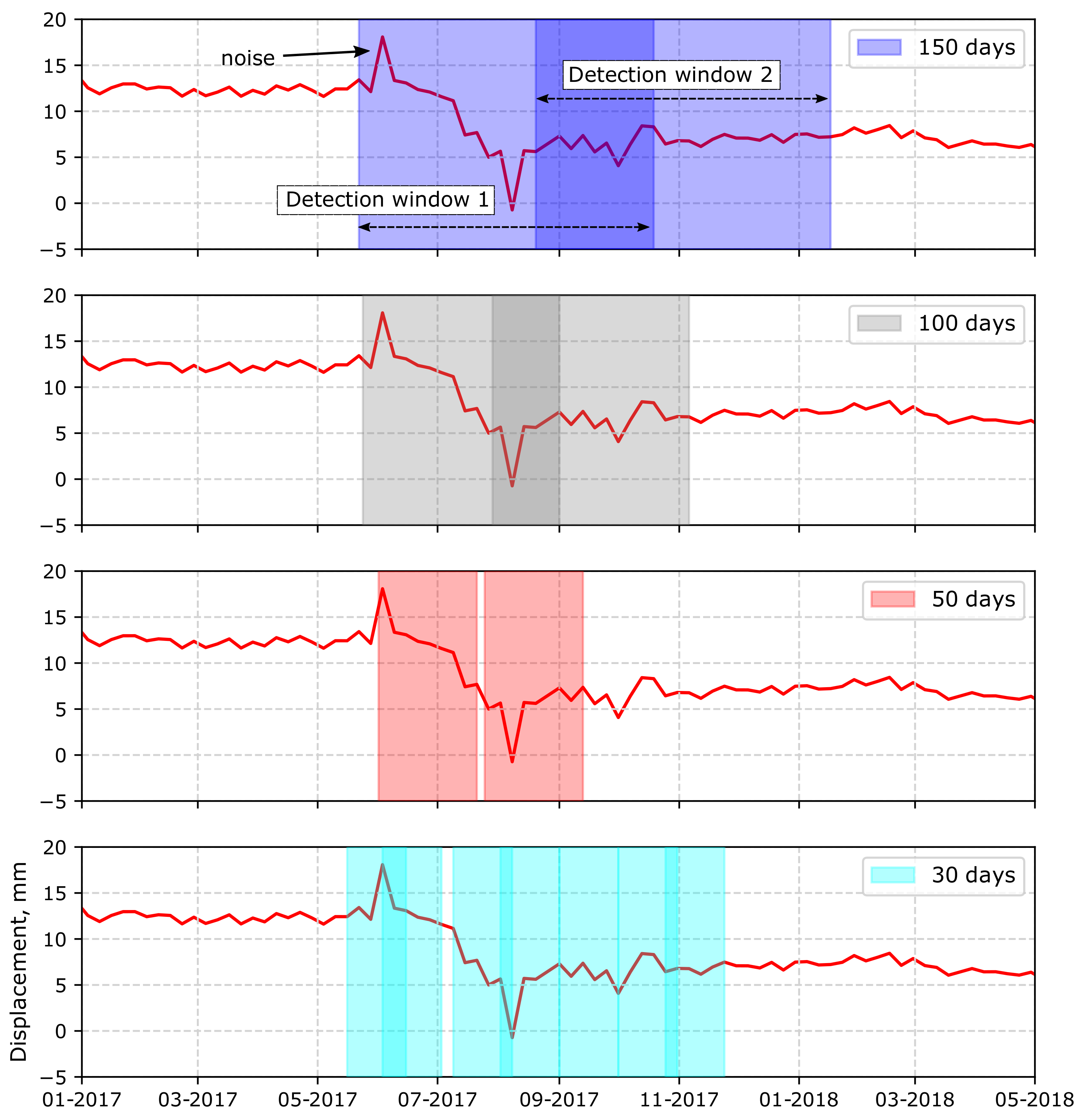
The choice of window size will determine the types of gradient changes that can be detected (Figure 9). Larger windows will be able to detect gradient changes that occur over a longer time period while shorter windows are more sensitive to noise. However larger windows may detect a gradient change too late to be of any use, unless it is a slow onset process. The window parameter therefore must be set based on the expected wavelength of the gradient changes we are trying to detect. A future improvement on the method could be to tune the gradient window through an iterative test to the application of interest in a specific region. Or to search for changes in several window sizes in order to capture different mechanisms at work.
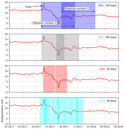
Figure 9.
Gradient detections using window sizes of 150 days, 100 days, 50 days and 30 days (top to bottom panels respectively). Our algorithm should detect two changes in the displacement gradient between 06-2017 and 09-2017. In all cases we do detect these two changes. However the smaller window size of 30 days is more prone to being affected by noise. For example, the noisy point at 06-2017 indicated on the top panel is detected by the smaller 30 day window, while the larger windows are less sensitive to this.
While the purpose of our method is rapid online detections with the aim of providing alerts for anomalous ground deformation, an additional benefit is that the algorithm works as an offline detector as well. This means that the method can be used to look for anomalous changes that have happened in the past given an existing InSAR time series (Figure 7).
Although we attempt to correct for signals caused by tropospheric delays, no currently available method can remove all of this noise, especially delays arising from the turbulent component of the atmosphere [42,43,44]. Previous studies have shown that in general, weather-model derived corrections can reduce the noise by 2–16% [45] resulting in an RMSE of around 2-3 cm [42] in individual interferograms. Atmospheric noise is generally uncorrelated in time [46]. These are seen as noisy peaks in the time series, and are the source of most of the variability in the displacement time series. The purpose of using a long 5 year displacement time series is to characterise the dispersion in the test statistic arising mostly due to this noise. Atmospheric noise-induced peaks in the time series are the main source of false positives in our offset detector. The gradient detector is less prone to these as long as the detection window is sufficiently large (Figure 9).
Caveats and Limitations
An important assumption in our method is that a sufficiently long time series already exists from which we can calculate the variance for our test statistic. Since the launch of Sentinel-1B in 2016 we now have an image every 6 days over Europe and every 12 days over the rest of the world. We assume that 90% of the existing time series (5 years of data for Sentinel-1) is sufficient to characterise the standard deviation of the difference series and the second derivative series, and this dispersion remains the same for new data points for online detections.
While SAR data collection by the Sentinel-1 constellation are now regular and consistent not all images might make it to the final time series. Occasionally, although this is now rare, an image might be corrupted or have missing bursts and so will not be usable in the time series analysis. In these cases there may be irregular gaps in the time series. This would not be a problem for offset detections as the difference calculations simply calculate the difference with previous measurements regardless of how far back that measurement was made. For the gradient change detection, each detection window requires a minimum of 2 measurements (preferably at least 5). So if there are large gaps in the time series there will be some null windows. Therefore large gaps are more of a problem for gradient change detections.
Unwrapping errors result in offsets in the time series. In our dataset we use the phase closure and bridging technique to correct unwrapping errors [28] in the interferograms. But this method cannot correct all errors, especially those in interferograms that do not undergo phase closure where unwrapping errors are harder to detect. For example the large jump in the middle of 2016 seen in all the pixel time series shown in Figure 7 is likely due to an unwrapping error. These errors could be minimised by including interferograms with longer temporal baselines that span across the times when low coherence is prevalent (e.g., the summer months), but how to do this in an automated way requires further research. In order to use our algorithm as the basis for a deformation early-warning system all attempts must be made to either correct unwrapping errors or remove interferograms that contain them before inverting the stack. Inversely, our method could be used to detect incorrectly unwrapped pixels. However more robust methods already exist in order to detect and correct these errors (e.g. [28,45]).
We show that by using a Gaussian blur we are able to filter out isolated detections, which we assume are false positives. The strength of this filter and the size of the kernel over which it is applied is context dependent. For example, if we are aiming to detect deformation that might precede landslide motion then the filter kernel window might need be smaller than the 200 m used in our case study. On the other hand, if we are interested in monitoring small sites with only few InSAR pixels (for example a bridge) then filtering will not be appropriate. In these cases the filter step can be skipped.
5. Conclusions
In this paper we present a statistical approach for detecting offsets and gradient changes in InSAR time series. A key requirement for both our offset and the gradient change detectors is that a sufficiently long time series already exists from which the standard deviation can be calculated. Over 5 years of data is now available from the Sentinel-1 satellite constellation. We believe that this is sufficient to determine the population standard deviation of the detection variables. We assume that this dispersion level remains the same for new additions to the time series, which enables online detection. Our offset detector assumes that the first, second and third difference series are stationary and identifies statistically significant peaks in these series. The gradient change detector uses rolling windows to identify statistically significant moments in the second derivative series. We exploit the high spatial resolution of Sentinel-1 data (approximate 5 by 15 m pixel size) and the spatial continuity of geophysical deformation signals to reduce false detections. Assuming that spatially isolated detections are false positives, we reduce these by using a Gaussian blur filter. In our test data stack over Hatfield Moors in the UK this resulted in an average reduction of 26% in the number of change detections. When combined with near-real time processing of InSAR data these detectors, particularly the gradient change, could be used to detect incipient ground deformation that precede dangerous geophysical phenomena, for example from landslides or volcanic eruptions. Alternatively it could be used to monitor for changes resulting from subsurface fluid injection/withdrawal processes.
Author Contributions
Conceptualization, E.H. and A.N.; methodology, E.H.; software, E.H. and A.N.; validation, A.N., L.B.; formal analysis, E.H.; investigation, E.H., L.B.; resources, C.J.; data curation, E.H., A.N.; writing—original draft preparation, E.H.; writing—review and editing, E.H., A.N., C.J., L.B.; visualization, E.H.; supervision, C.J.; project administration, E.H..; funding acquisition, E.H., A.N. All authors have read and agreed to the published version of the manuscript.
Funding
The research for technique development and testing was funded by the Innovation Flexible Fund (IFF) at the British Geological Survey. The data processing was supported by the ACT-2 SENSE project. SENSE (Assuring integrity of CO2 storage sites through ground surface monitoring) project No. 299664, has been subsidized through ACT (EC Project no. 691712) by Gassnova, Norway, United Kingdom Department for Business, Energy and Industrial Strategy, Forschungszentrum Jülich GMBH, Projektträger Jülich, Germany, The French Agency for the Environment and Energy Management, The United States Department of Energy and State Research Agency, Spain. Additional support from Equinor and Quad Geometrics and permission to use data from the Krechba Field by In Salah Gas JV are appreciated.
Data Availability Statement
Not applicable.
Acknowledgments
We gratefully acknowledge helpful discussions with colleagues during the early stages of this research, particularly Karsten Spaans at the University of Leeds. Thanks to Piyush Agram for the tip on using numpy stride tricks to improve efficiency. We would like to thank the European Space Agency for free provision of the Sentinel-1 radar imagery. The authors publish with the permission of the Executive Director of the British Geological Survey.
Conflicts of Interest
The authors declare no conflict of interest. The funders had no role in the design of the study; in the collection, analyses, or interpretation of data; in the writing of the manuscript, or in the decision to publish the results.
References
- Biggs, J.; Wright, T.J. How satellite InSAR has grown from opportunistic science to routine monitoring over the last decade. Nat. Commun. 2020, 11, 1–4. [Google Scholar] [CrossRef]
- Minh, D.H.T.; Hanssen, R.; Rocca, F. Radar Interferometry: 20 Years of Development in Time Series Techniques and Future Perspectives. Remote Sens. 2020, 12, 1364. [Google Scholar] [CrossRef]
- Ebmeier, S.K. Application of independent component analysis to multitemporal InSAR data with volcanic case studies. J. Geophys. Res. Solid Earth 2016, 121. [Google Scholar] [CrossRef]
- Bonì, R.; Bosino, A.; Meisina, C.; Novellino, A.; Bateson, L.; McCormack, H. A Methodology to Detect and Characterize Uplift Phenomena in Urban Areas Using Sentinel-1 Data. Remote Sens. 2018, 10, 607. [Google Scholar] [CrossRef]
- Gaddes, M.; Hooper, A.; Bagnardi, M.; Inman, H.; Albino, F. Blind signal separation methods for InSAR: The potential to automatically detect and monitor signals of volcanic deformation. J. Geophys. Res. Solid Earth 2018, 123, 10–226. [Google Scholar] [CrossRef]
- Jordan, C.; Bateson, L.; Novellino, A. Environmental baseline monitoring for shale-gas development: Insights for monitoring ground motion using InSAR analysis. Sci. Total. Environ. 2019, 696, 134075. [Google Scholar] [CrossRef]
- Van de Kerkhof, B.; Pankratius, V.; Chang, L.; van Swol, R.; Hanssen, R.F. Individual Scatterer Model Learning for Satellite Interferometry. IEEE Trans. Geosci. Remote Sens. 2020, 58, 1273–1280. [Google Scholar] [CrossRef]
- Albino, F.; Biggs, J.; Yu, C.; Li, Z. Automated Methods for Detecting Volcanic Deformation Using Sentinel-1 InSAR Time Series Illustrated by the 2017–2018 Unrest at Agung, Indonesia. J. Geophys. Res. Solid Earth 2020, 125, e2019JB017908. [Google Scholar] [CrossRef]
- Maubant, L.; Pathier, E.; Daout, S.; Radiguet, M.; Doin, M.P.; Kazachkina, E.; Kostoglodov, V.; Cotte, N.; Walpersdorf, A. Independent component analysis and parametric approach for source separation in InSAR time series at regional scale: Application to the 2017–2018 Slow Slip Event in Guerrero (Mexico). J. Geophys. Res. Solid Earth 2020, 125, e2019JB018187. [Google Scholar] [CrossRef]
- Osmanoğlu, B.; Dixon, T.H.; Wdowinski, S.; Cabral-Cano, E.; Jiang, Y. Mexico City subsidence observed with persistent scatterer InSAR. Int. J. Appl. Earth Obs. Geoinf. 2011, 13, 1–12. [Google Scholar] [CrossRef]
- Baer, G.; Schattner, U.; Wachs, D.; Sandwell, D.; Wdowinski, S.; Frydman, S. The lowest place on Earth is subsiding – An InSAR (interferometric synthetic aperture radar) perspective. Geol. Soc. Am. Bull. 2002, 114, 12–23. [Google Scholar] [CrossRef]
- Ebmeier, S.K.; Andrews, B.J.; Araya, M.C.; Arnold, D.W.D.; Biggs, J.; Cooper, C.; Cottrell, E.E.A. Synthesis of global satellite observations of magmatic and volcanic deformation: Implications for volcano monitoring and the lateral extent of magmatic domains. J. Appl. Volcanol. 2018, 7. [Google Scholar] [CrossRef]
- Gama, F.F.; Mura, J.C.; Paradella, W.R.; de Oliveira, C.G. Deformations Prior to the Brumadinho Dam Collapse Revealed by Sentinel-1 InSAR Data Using SBAS and PSI Techniques. Remote Sens. 2020, 12, 3664. [Google Scholar] [CrossRef]
- Aminikhanghahi, S.; Cook, D.J. A survey of methods for time series change point detection. Knowl. Inf. Syst. 2017, 51, 339–367. [Google Scholar] [CrossRef]
- Oh, K.J.; Kim, K.j. Analyzing stock market tick data using piecewise nonlinear model. Expert Syst. Appl. 2002, 22, 249–255. [Google Scholar] [CrossRef]
- Miyazaki, B.; Izumi, K.; Toriumi, F.; Takahashi, R. Change detection of orders in stock markets using a Gaussian mixture model. Intell. Syst. Account. Financ. Manag. 2014, 21, 169–191. [Google Scholar] [CrossRef]
- Berti, M.; Corsini, A.; Franceschini, S.; Iannacone, J. Automated classification of Persistent Scatterers Interferometry time series. Nat. Hazards Earth Syst. Sci. 2013, 13, 1945–1958. [Google Scholar] [CrossRef]
- Anantrasirichai, N.; Biggs, J.; Albino, F.; Bull, D. A deep learning approach to detecting volcano deformation from satellite imagery using synthetic datasets. Remote Sens. Environ. 2019, 230, 111179. [Google Scholar] [CrossRef]
- Anantrasirichai, N.; Biggs, J.; Albino, F.; Bull, D. The Application of Convolutional Neural Networks to Detect Slow, Sustained Deformation in InSAR Time Series. Geophys. Res. Lett. 2019, 46, 11850–11858. [Google Scholar] [CrossRef]
- Anantrasirichai, N.; Biggs, J.; Kelevitz, K.; Sadeghi, Z.; Wright, T.; Thompson, J.; Achim, A.M.; Bull, D. Detecting Ground Deformation in the Built Environment using Sparse Satellite InSAR data with a Convolutional Neural Network. IEEE Trans. Geosci. Remote Sens. 2020, 59, 2940–2950. [Google Scholar] [CrossRef]
- Gaddes, M.; Hooper, A.; Bagnardi, M. Using machine learning to automatically detect volcanic unrest in a time series of interferograms. J. Geophys. Res. Solid Earth 2019, 124, 12304–12322. [Google Scholar] [CrossRef]
- Malinowski, R.; Lewiński, S.; Rybicki, M.; Gromny, E.; Jenerowicz, M.; Krupiński, M.; Nowakowski, A.; Wojtkowski, C.; Krupiński, M.; Krätzschmar, E.; et al. Automated Production of a Land Cover/Use Map of Europe Based on Sentinel-2 Imagery. Remote Sens. 2020, 12, 3523. [Google Scholar] [CrossRef]
- Natural England. Humberhead Peatlands. Available online: https://www.humberheadpeatlands.org.uk (accessed on 15 December 2020).
- Scottish Power. Hatfield Moors Gas Storage Facility: Site Information. Available online: https://www.scottishpower.com/userfiles/file/Hatfield-Site-Information-2014.pdf (accessed on 15 December 2020).
- Accelerating CCS Technologies, EU Horizon 2020. SENSE Project: Assuring Integrity of CO2 Storage Sites through Ground Surface Monitoring. Available online: https://sense-act.eu (accessed on 16 December 2020).
- Rosen, P.A.; Gurrola, E.; Sacco, G.F.; Zebker, H. The InSAR Scientific Computing environment. In Proceedings of the 9th European Conference on Synthetic Aperture Radar (EUSAR 2012), Nuremberg, Germany, 23–26 April 2012; pp. 730–733. [Google Scholar]
- Rosen, P.A.; Gurrola, E.M.; Agram, P.; Cohen, J.; Lavalle, M.; Riel, B.V.; Fattahi, H.; Bekaert, D.P.S.; Aivazis, M.A.; Simons, M.; et al. The Interferometric Synthetic Aperture Radar Scientific Computing Environment (ISCE2), v2.3.3. Available online: https://github.com/isce-framework/isce2 (accessed on 1 June 2020).
- Yunjun, Z.; Fattahi, H.; Amelung, F. Small baseline InSAR time series analysis: Unwrapping error correction and noise reduction. Comput. Geosci. 2019, 133, 104331. [Google Scholar] [CrossRef]
- Yunjun, Z.; Fattahi, H.; Amelung, F. The Miami INsar Time-Series Software in PYthon (MintPy), v1.2.2. Available online: https://github.com/insarlab/MintPy (accessed on 1 June 2020).
- Jolivet, R.; Agram, P.S.; Lin, N.Y.; Simons, M.; Doin, M.P.; Peltzer, G.; Li, Z. Improving InSAR geodesy using global atmospheric models. J. Geophys. Res. Solid Earth 2014, 119, 2324–2341. [Google Scholar] [CrossRef]
- Farr, T.G.; Rosen, P.A.; Caro, E.; Crippen, R.; Duren, R.; Hensley, S.; Kobrick, M.; Paller, M.; Rodriguez, E.; Roth, L.; et al. The shuttle radar topography mission. Rev. Geophys. 2007, 45. [Google Scholar] [CrossRef]
- Chen, C.W.; Zebker, H.A. Phase unwrapping for large SAR interferograms: Statistical segmentation and generalized network models. IEEE Trans. Geosci. Remote Sens. 2002, 40, 1709–1719. [Google Scholar] [CrossRef]
- Shumway, R.H.; Stoffer, D.S. Time Series Analysis and Its Applications: With R Examples; Springer: Berlin/Heidelberg, Germany, 2017. [Google Scholar]
- Prabhakaran, S. Augmented Dickey Fuller Test (ADF Test)—Must Read Guide. Available online: https://www.machinelearningplus.com/time-series/augmented-dickey-fuller-test/ (accessed on 27 January 2021).
- Hyndman, R.; Athanasopoulos, G. Forecasting: Principles and Practice, 2nd ed. Available online: https://otexts.com/fpp2/ (accessed on 21 January 2021).
- Derrick, B. How to compare the means of two samples that include paired observations and independent observations: A companion to Derrick, Russ, Toher and White (2017). Quant. Methods Psychol. 2017, 13, 120–126. [Google Scholar] [CrossRef]
- Berg, S. Multidimensional Rolling Window for Numpy. Available online: https://gist.github.com/seberg/3866040 (accessed on 27 January 2020).
- Zhou, Z.; Li, Z.; Waldron, S.; Tanaka, A. InSAR Time Series Analysis of L-band data for understanding tropical peatland degradation and restoration. Remote Sens. 2019, 11, 2592. [Google Scholar] [CrossRef]
- Alshammari, L.; Boyd, D.S.; Sowter, A.; Marshall, C.; Andersen, R.; Gilbert, P.; Marsh, S.; Large, D.J. Use of surface motion characteristics determined by InSAR to assess peatland condition. J. Geophys. Res. Biogeosci. 2020, 125, e2018JG004953. [Google Scholar] [CrossRef]
- Sun, J.; Wauthier, C.; Stephens, K.; Gervais, M.; Cervone, G.; La Femina, P.; Higgins, M. Automatic Detection of Volcanic Surface Deformation Using Deep Learning. J. Geophys. Res. Solid Earth 2020, 125, e2020JB019840. [Google Scholar] [CrossRef]
- Raspini, F.; Bianchini, S.; Ciampalini, A.; Del Soldato, M.; Solari, L.; Novali, F.; Del Conte, S.; Rucci, A.; Ferretti, A.; Casagli, N. Continuous, semi-automatic monitoring of ground deformation using Sentinel-1 satellites. Sci. Rep. 2018, 8, 1–11. [Google Scholar] [CrossRef]
- Bekaert, D.; Walters, R.; Wright, T.; Hooper, A.; Parker, D. Statistical comparison of InSAR tropospheric correction techniques. Remote Sens. Environ. 2015, 170, 40–47. [Google Scholar] [CrossRef]
- Murray, K.D.; Bekaert, D.P.; Lohman, R.B. Tropospheric corrections for InSAR: Statistical assessments and applications to the Central United States and Mexico. Remote Sens. Environ. 2019, 232, 111326. [Google Scholar] [CrossRef]
- Haji-Aghajany, S.; Amerian, Y. Assessment of InSAR tropospheric signal correction methods. J. Appl. Remote Sens. 2020, 14, 044503. [Google Scholar] [CrossRef]
- Hussain, E.; Hooper, A.; Wright, T.J.; Walters, R.J.; Bekaert, D.P. Interseismic strain accumulation across the central North Anatolian Fault from iteratively unwrapped InSAR measurements. J. Geophys. Res. Solid Earth 2016, 121, 9000–9019. [Google Scholar] [CrossRef]
- Hanssen, R. Remote sensing and digital image processing. Radar Interferom. Data Interpret. Error Anal. Earth Environ. Sci. 2001, 2, 200–210. [Google Scholar]
Publisher’s Note: MDPI stays neutral with regard to jurisdictional claims in published maps and institutional affiliations. |
© 2021 by the authors. Licensee MDPI, Basel, Switzerland. This article is an open access article distributed under the terms and conditions of the Creative Commons Attribution (CC BY) license (https://creativecommons.org/licenses/by/4.0/).

