Article

An Instance Segmentation Based Framework for Large-Sized High-Resolution Remote Sensing Images Registration

1
Changchun Institute of Optics, Fine Mechanics and Physics, Chinese Academy of Sciences, Changchun 130033, China
2
University of Chinese Academy of Sciences, Beijing 100049, China
3
Key Laboratory of Satellite Remote Sensing Application Technology of Jilin Province, Chang Guang Satellite Technology Company Ltd., Changchun 130000, China
4
Shanghai Electro-Mechanical Engineering Institute, Shanghai 201109, China
*
Author to whom correspondence should be addressed.
Remote Sens. 2021, 13(9), 1657; https://doi.org/10.3390/rs13091657
Submission received: 3 March 2021 / Revised: 20 April 2021 / Accepted: 21 April 2021 / Published: 23 April 2021

Abstract

:
Feature-based remote sensing image registration methods have achieved great accomplishments. However, they have faced some limitations of applicability, automation, accuracy, efficiency, and robustness for large high-resolution remote sensing image registration. To address the above issues, we propose a novel instance segmentation based registration framework specifically for large-sized high-resolution remote sensing images. First, we design an instance segmentation model based on a convolutional neural network (CNN), which can efficiently extract fine-grained instances as the deep features for local area matching. Then, a feature-based method combined with the instance segmentation results is adopted to acquire more accurate local feature matching. Finally, multi-constraints based on the instance segmentation results are introduced to work on the outlier removal. In the experiments of high-resolution remote sensing image registration, the proposal effectively copes with the circumstance of the sensed image with poor positioning accuracy. In addition, the method achieves superior accuracy and competitive robustness compared with state-of-the-art feature-based methods, while being rather efficient.

Graphical Abstract

1. Introduction

The process of image registration is to find the pixel space mapping relationship between the sensed and reference images, thereby, transforming the sensed image into the geometric coordinate system of the reference image. The sensed and reference images are usually the same scene taken by different times, sensors, or viewpoints [1,2,3]. Registration is a significant task in the application of remote sensing images, and feature-based methods are often recommended to achieve it due to their effectiveness [4]. Feature-based methods usually consist of three key steps: key point detection and feature description, feature matching, and outlier removal [5]. Specifically, key point detection and feature description refer to searching the distinctive points in an image and representing them by descriptors. The process performs through algorithms, such as scale-invariant feature transform (SIFT) [6], speeded up robust features (SURF) [7], oriented FAST and rotated BRIEF (ORB) [8], accelerated KAZE features (AKAZE) [9], etc. Feature matching refers to matching the key points based on the particular similarity measures (such as Euclidean distance, etc.) of their feature vectors. Outlier removal refers to the use of algorithms, such as random sample consensus (RANSAC) [10], to eliminate the false matches.
In recent years, continuous breakthroughs in satellite technology have made the spatial resolution of remote sensing images increasingly improved, so the image pixel size of the same shooting area also becomes larger, and the application of high-resolution remote sensing images is more widespread [11]. Combining the definitions in References [5,11,12], this paper considers the spatial resolution higher than 1 m (or the ground sampling distance less than 1 m) is high resolution, and the number of pixels greater than 10,000 × 10,000 is a large size. State-of-the-art feature-based remote sensing image registration methods have achieved a great accomplishment. However, they have faced some limitations of applicability, automation, accuracy, efficiency, and robustness for large high-resolution remote sensing images, which will be discussed in detail in Section 2. To address the above issues, we propose a novel registration framework based on instance segmentation in this paper. First, the approach makes full use of the convolutional neural network (CNN) to extract the concerned instances in the sensed and reference images. An instance matching strategy that does not depend on positioning accuracy is applied to match the local areas. Next, a feature-based method combined with instance segmentation results is adopted to acquire more accurate, local feature matching. Finally, multi-constraints are used to work on outlier removal and the registration is achieved. There are two main contributions of this work.
  • We propose an automatic registration framework specifically for large high-resolution remote sensing images. The method enhances the applicability of the sensed image with poor positioning accuracy, improves the accuracy and robustness of registration, and remains rather efficient. Furthermore, the framework supports embedding various feature-based methods to satisfy the requirement for more flexible applications. The above points will be illustrated in detail in Section 3 and Section 4.
  • We propose an instance segmentation algorithm based on deep learning to achieve fine-grained and efficient extraction of the concerned objects for the registration framework, which will be introduced in Section 3. Even if it is not used for subsequent registration, the independent application of this algorithm to intelligent interpretation of remote sensing images also has broad significance and value.
The rest of this paper is organized as follows. Section 2 introduces the related works and analyzes their limitations. The proposed method is detailed in Section 3. Experimental results are illustrated in Section 4. Finally, Section 5 draws the conclusions of this paper.

2. Related Works

In this section, we briefly introduce the state-of-the-art feature-based registration methods for remote sensing images. In addition, we analyze the limitations of related works applied to large high-resolution remote sensing images.

2.1. Feature-Based Methods for Remote Sensing Image Registration

Distinctive image features are usually described by about two categories: hand-crafted features and deep features [4]. In view of the characteristics of remote sensing images, scholars have made various improvements to the classic hand-crafted, feature-based methods to propose new feature descriptors or feature matching strategies [11,12,13,14,15,16,17,18,19,20,21,22,23,24]. For example, Morel et al. [11] introduced transition tilt to measure the amount of distortion from one view to another, and proposed a modified SIFT feature, Affine-SIFT (ASIFT), which is proved to be a fully affine invariant. Dellinger et al. [12] presented a new gradient calculation, which is robust to speckle noise, and used it to adapt the steps of the SIFT algorithm, which introduced the SAR-SIFT for synthetic aperture radar (SAR) image registration. Ma et al. [13] proposed a modified SIFT feature, PSO-SIFT, which introduces a new gradient definition to overcome the difference of intensity between the remote sensing images, as well as an enhanced feature matching method to increase the number of correct correspondences. Ye et al. [14] proposed the channel features of orientated gradients (CFOG), which is an extension of the histogram of the oriented gradient (HOG) descriptor and outperforms both in-matching performance and computational efficiency. Huo et al. [15] introduced a coarse-to-fine strategy for large-sized, very high-resolution, remote sensing image registration. The original image pairs were reduced to a small size and low resolution by direct down sampling, and SIFT was implemented to the down-sampled images to obtain the global matching and coarse transformation. Then, the coarsely aligned original images were divided into corresponding block pairs and block-wise SIFT was applied to reach the refinement. Sedaghat et al. [17] introduced a uniform robust selection strategy of SIFT features in the full distribution of location and scale where the feature qualities are quarantined based on the stability and distinctiveness constraints. Goncalves [18] et al. combined image segmentation and SIFT to propose a remote sensing image registration scheme, which allowed for an accurate obtention of tie points. Gong et al. [19] proposed a coarse-to-fine scheme for remote sensing image registration, which implemented the coarse registration by SIFT and the fine-tuning by the maximization of mutual information. Kupfer et al. [21] presented a mode seeking SIFT (MS-SIFT) method, which exploits the scale, orientation, and position associated with the SIFT feature to refine the result by eliminating outliers.
However, hand-crafted features are designed based on careful engineering and domain knowledge, which makes them somewhat specific but less generalized [25]. Moreover, hand-crafted features are usually low-level features of edge, texture, corner, and the statistical information of gradient, but lack high-level semantic information. Therefore, they solely perform well on the specific local areas while they cannot cope with the global complexity of remote sensing images [4,5,25]. Then, some research studies put effort on automatically acquiring more expressive deep features through deep learning for registration. For instance, Wang et al. [25] first adopted SIFT to detect key points and obtained patches centered on them. Then, a deep neural network (DNN) was trained to learn the matching label of an input patch pair vector. Next, patch pairs from the sensed and reference images were input to the trained DNN to determine whether they match, thus, acquiring matching point pairs. Finally, the transform matrix was computed after outlier removal. Zhu et al. [5] proposed a two-branch Siamese convolutional deep belief network (CDBN). The patches centered at the key points were entered into the CDBN to learn discriminative feature representations for patch matching, while the key points were detected by Difference of Gaussian (DoG). The size of each patch was determined by the scale of its central key point through an adaptive sample selection strategy, and two matching strategies are designed to improve the efficiency and accuracy. Ma et al. [4] presented a two-step coarse-to-fine registration method based on CNN. In the first step, the deep features of sensed and reference images were extracted from the deep feature maps of CNN, and were matched by the Euclidean distance to calculate the approximate spatial relationship. For the second step, a classic feature-based method, such as SIFT, was applied to the local areas to refine the result.

2.2. Limitations of Related Works for Large-Sized High-Resolution Remote Sensing Images

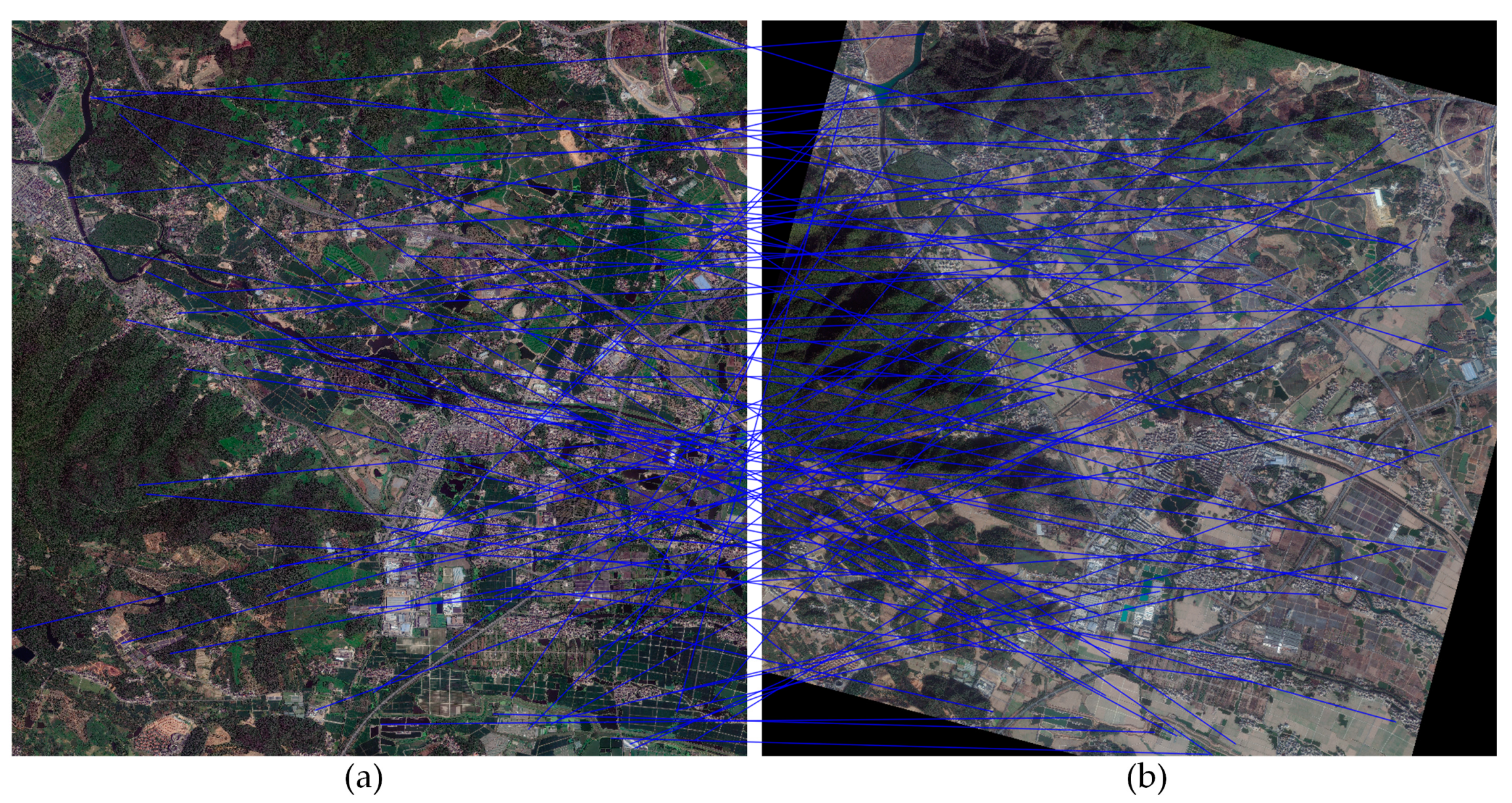
In the previously mentioned related works [4,5,11,12,13,14,15,16,17,18,19,20,21,22,23,24,25], the test data of References [5,14,15] are large, high-resolution, remote sensing images (spatial resolution is higher than 1 m, and the number of pixels is greater than 10,000 × 10,000). In other works [4,11,12,13,16,17,18,19,20,21,22,23,24,25], the number of pixels of the test data are basically less than 800 × 800, and the spatial resolutions are between 10 m and 100 m. Due to the limitation of hardware computing power, it is hard to directly use the entire large-sized, high-resolution, remote sensing images as inputs. Therefore, the methods proposed in References [5,14,15] align the sensed and reference images, according to their geographic spatial coordinates and divide them into blocks, and then perform their respective procedures between the corresponding block pairs. We believe the methods proposed in References [4,11,12,13,16,17,18,19,20,21,22,23,24,25] should adopt similar approaches when being applied to large-sized, high-resolution remote sensing images. However, when the positioning accuracy of the sensed image is poor, there is no actual overlapping area between its block and the corresponding reference block, which is diagramed as in Figure 1. In Figure 1, (a) is the sensed image whose positioning accuracy is poor, and (b) is the reference image in the same geographic area. The same color indicates the corresponding block pair, which shows that there are basically no overlapping areas between the pairs. Therefore, it is impossible to match the correct key points between the corresponding blocks in theory. The related works except References [5,15,25] rely on the positioning accuracy to obtain the corresponding block pairs and are not applicable in this case. The method [15] first down-samples the original images for coarse registration, and then obtains the corresponding block pairs. However, the SIFT matching may fail when the down-sampling ratio is too large [15], and SIFT does not work well for the global complexity of remote sensing images [25]. The method [5] first performs iterative manual coarse registration of the original images to a certain accuracy, which is not automatic. The method [25] to obtain the corresponding block pairs does not rely on geographic areas but on SIFT key points. However, the number of key points in large, high-resolution remote sensing images is very large (see Figure 2 below), and the method uses brute force matching for block pair generation, so it is almost infeasible in this case. Furthermore, even if the computing power allows the registration of the images, the number of key points will be far greater than the dimension of the descriptor. At this time, the features will be overwhelmed by the large number of samples and lose meaning, resulting in a complete failure of subsequent matching, which is shown in Figure 2. Figure 2 shows the registration result of the entire sensed image (left, size of 10,000 × 10,000 pixels) and reference image (right, size of 10,000 × 10,000 pixels). The numbers of key points detected by SIFT are about 2.8 million (left) and 1 million (right), respectively. The dimension of the SIFT descriptor is 128. Each key point has too many similarities in such a large sample size, thus, losing its uniqueness. We randomly select 100 matches for drawing, and they are basically all wrong.
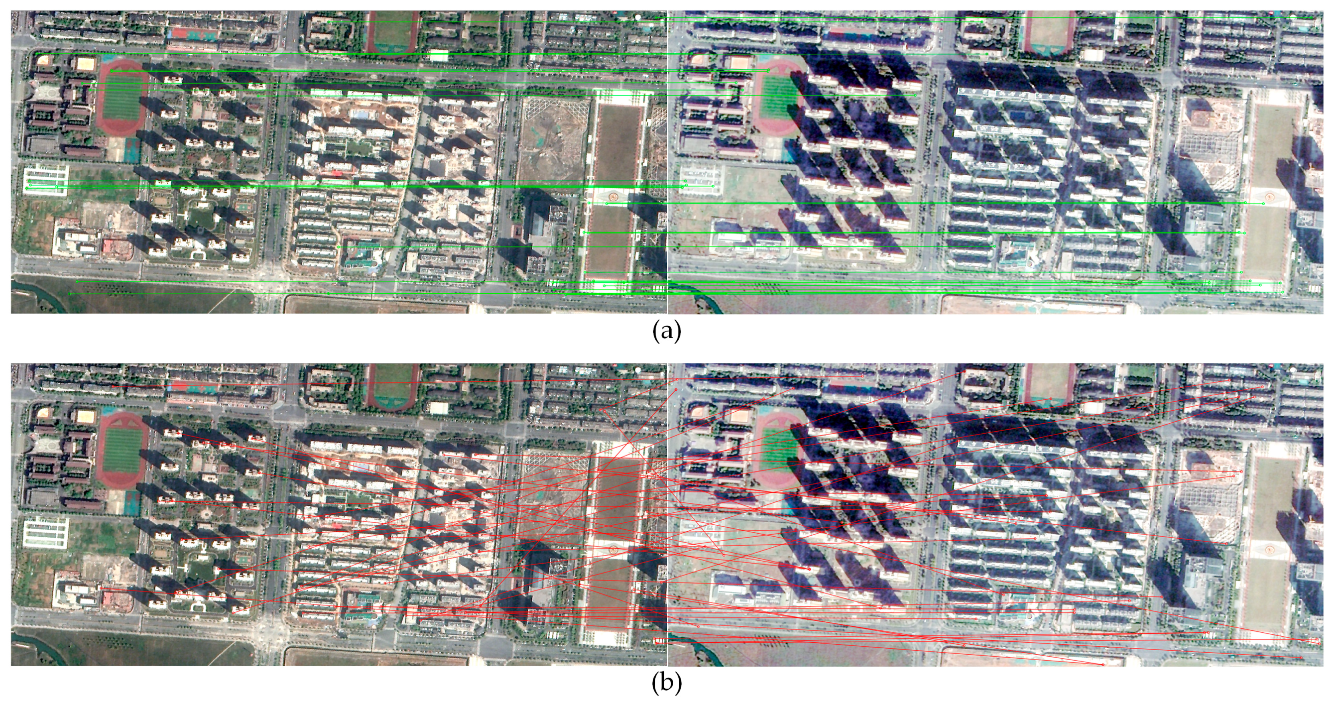
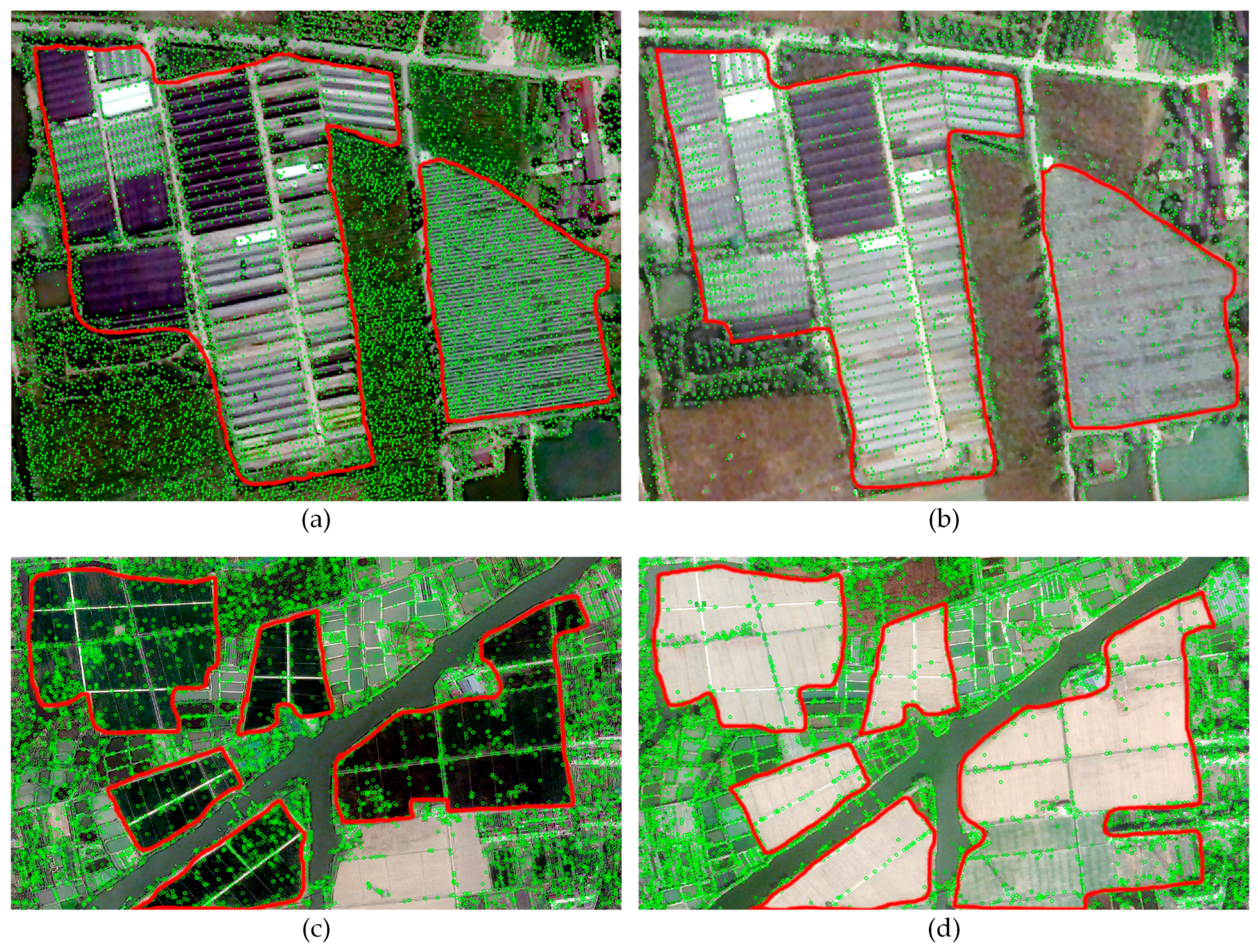
In addition, high-resolution remote sensing images contain more clear and detailed ground objects, while using some of them for registration is counterproductive. This problem has not been studied in related works. For example, the buildings in the images will be deformed as the off-nadir angle changes [26], which is shown in Figure 3. We register a pair of images of the same area containing buildings by SIFT. Through manual inspection, we find that 29 pairs of key points are correctly matched, of which 25 pairs are on the ground and four pairs are on the buildings. More than 100 pairs of key points are mismatched. We randomly select 100 of them for statistics and find that 60 pairs are on the buildings and 40 pairs are on the ground. We diagram the correct matches on the ground in Figure 3a and the mismatches on the buildings in Figure 3b, respectively. The example shows that, if the key points on the buildings participate in registration, it will seriously reduce the accuracy. In other words, we prefer to match the key points on the ground rather than on the buildings. Another example, as illustrated in Figure 4, (a) and (b) are the summer and winter images of the same area containing greenhouses (within the red lines), respectively. (c) and (d) are the summer and winter images of the same area containing ponds (within the red lines), respectively. The green dots are the key points detected by SIFT and many of them are on the greenhouses and ponds. However, the greenhouses and ponds have changed a lot in different seasons (such as shape, color, material, etc.) or even cease to exist, and they are easy to form key points in the images due to sudden changes in brightness caused by reflections. Therefore, the key points on the greenhouses and ponds are temporary rather than fixed. That is, these key points are detected under specific shooting time and conditions, and they are difficult to be reproduce in another scene, thus, being meaningless for registration. Furthermore, if these key points are involved in registration, the correct matching ratio will be diluted and the accuracy will be reduced.
Moreover, the related works except References [4,5,25] perform feature-based registration processes on all parts of the images. For large, high-resolution remote sensing images, the computational and storage costs of feature-based methods are very huge [15], thus, resulting in low efficiency.
In summary, related works have faced some limitations in the application of large-sized, high-resolution remote sensing images. The first is inapplicability or non-automatic due to the sensed image with poor positioning accuracy. The second is the loss of accuracy or the poor robustness due to some certain ground objects in the images. The third is the inefficiency caused by a huge amount of calculation.

3. Proposed Methods

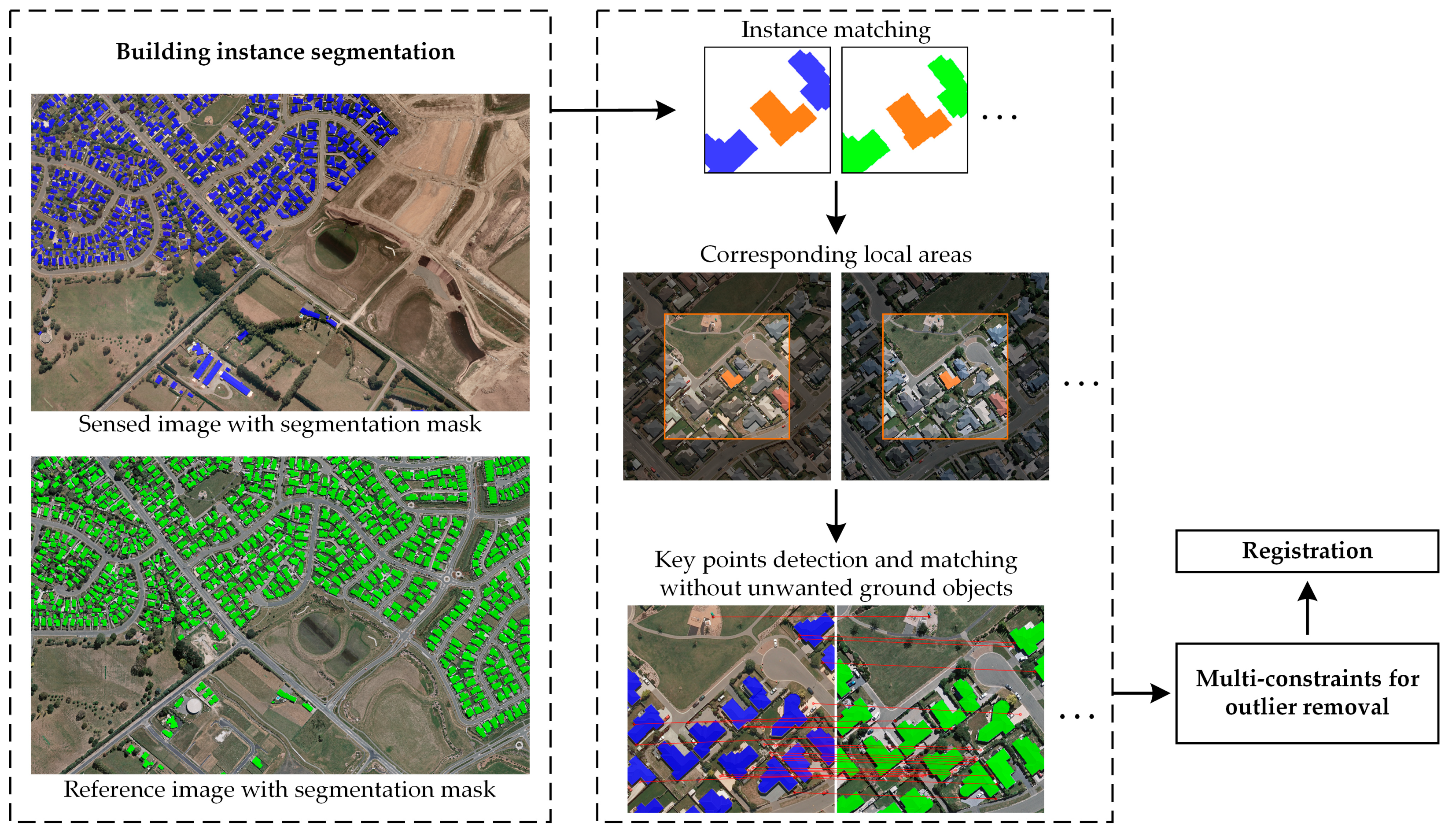
Addressing the above issues, we propose a novel framework for large, high-resolution, remote sensing image automatic registration. Since hand-crafted features perform well on the local areas but have poor global performance, we first use deep features to match the local areas between the global images, and then use hand-crafted features to match the key points between the local areas. Specifically, we propose an instance segmentation CNN model specifically for high-resolution, remote sensing images to acquire the deep features. The instance segmentation results are the generalized deep features, which is different from the related works whose deep features are pure feature vectors. The instance segmentation based framework has better generalization ability and robustness than related works. In particular, the methods proposed in References [5,25] train deep learning models to predict the matching labels of the input image block pairs, and select training samples on the sensed and reference images. Therefore, each registration task requires reselecting the samples and retraining the model, and the deep learning model trained each time cannot be applied to other tasks. The method [4] randomly selects 1000 disjoint block pairs from 10 multimodal remote sensing images of the same scene as 1000 categories to train a CNN for classification. However, this kind of category selection is purposeless, and the categories do not have specific and independent characteristics. In addition, remote sensing scenes are ever-changing while a single scene cannot provide representative samples. In contrast, we choose several categories of samples that contain specific and independent characteristics to train the instance segmentation model, and our training data comes from a variety of remote sensing scenes. Therefore, our trained model can be used repeatedly for each registration task, thus, having better generalization ability and robustness. In fact, the deep learning models of the methods proposed in References [4,5,25] are only intermediate results of the registration tasks without practical significance. In contrast, our model is the result of a standard instance segmentation task for extracting concerned ground objects, so it is also meaningful and valuable to be applied independently to the remote sensing image’s intelligent interpretation. Considering that some ground objects affect the registration accuracy as discussed in Section 2, we select them as the concerned instances to extract from the sensed and reference images, and the proposed framework is depicted as in Figure 5. Taking the instance segmentation of buildings as an example, according to the segmentation masks (the blue and green ones), we design an instance matching strategy, which uses an image processing approach and does not rely on geospatial information, thus, effectively coping with the problem of the sensed image with poor positioning accuracy. The orange ones indicate a pair of matching instances, and we obtain the corresponding local areas by their positions in the images. Then, we mask out the buildings in the local areas and perform a feature-based method to acquire more accurate matching key points between the local areas. Finally, we introduce a multi-constraints strategy to work on outlier removal. Our framework is two-step rather than coarse-to-fine as in References [4,15,19]. That is, we do not coarsely register first and then refine but register only once, which simplifies the intermediate process. In addition, we only perform a feature-based registration method between the matching local areas, which greatly reduces the amount of calculation and improves efficiency. The feature-based method is performed in an independent step, so it can be selected flexibly. Moreover, the automation of our method is of great significance for engineering applications [4,14,19]. The proposed instance segmentation model, instance matching, and outlier removal strategies are described in detail below.

3.1. Single-Stage Fine-Grained Instance Segmentation Network for High-Resolution Remote Sensing Images

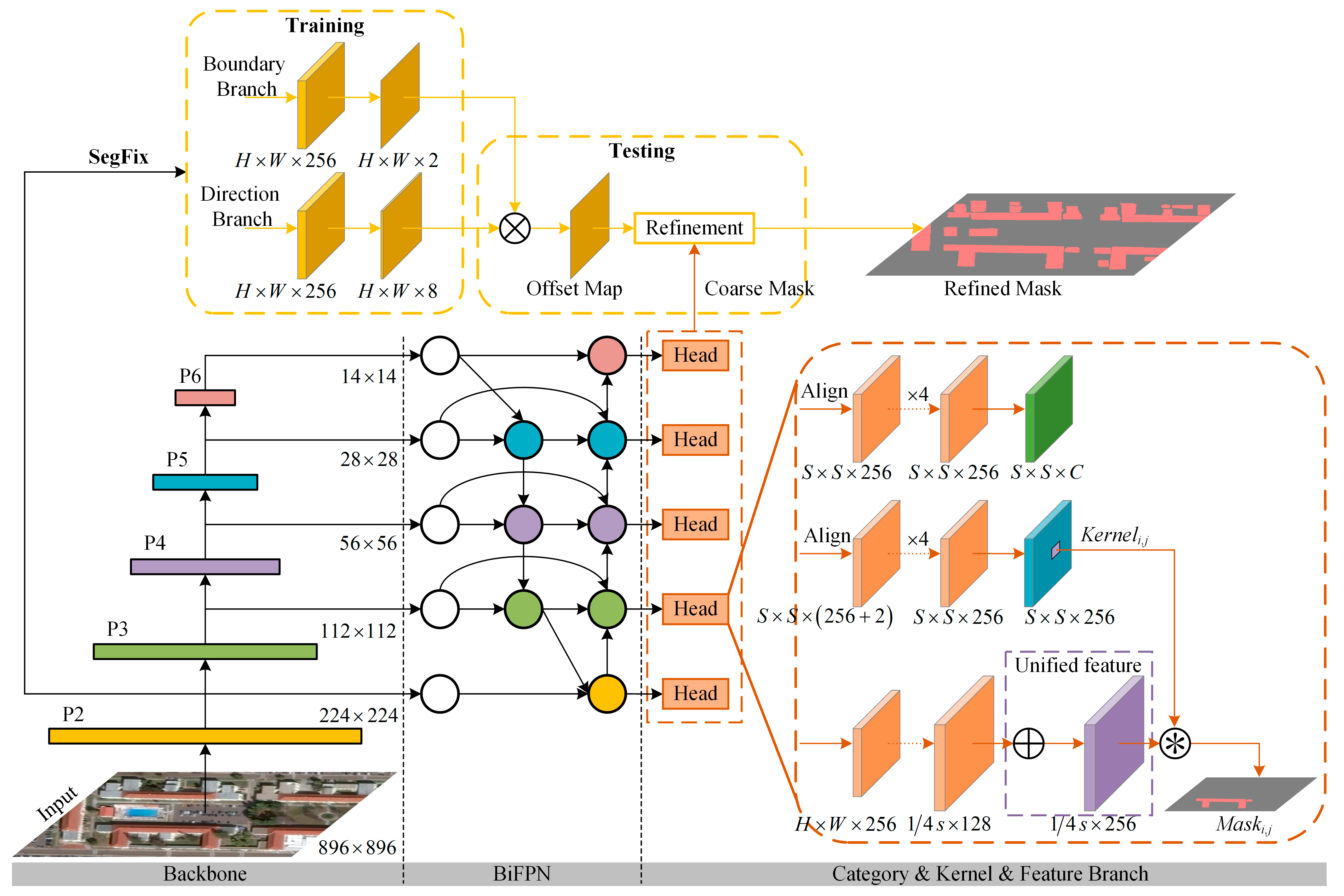
Instance segmentation is a classic task in computer vision [27], which detects the concerned objects from the image and segments the instance foregrounds. With the rise of deep learning technology, instance segmentation algorithms based on CNN [28,29,30,31,32,33] have received more attention and research, and have played an increasingly important role in remote sensing image interpretation [34,35,36,37]. Since the subsequent instance matching step rely heavily on fine segmentation boundaries, and in order to improve the efficiency of instance segmentation, we propose a single-stage, fine-grained (SSFG) instance segmentation network for high-resolution remote sensing images, whose structure is shown in Figure 6 and the main points are as follows.
  • Backbone of high-resolution feature maps. With the pooling of CNN, the loss of object features (especially boundary features) is severe, so that the subsequent up-sampling generates a segmentation mask with poor object boundary fineness. We use HRNetV2p [41] as the backbone of the SSFG, which enables the feature maps to maintain a high-resolution representation during the feature extraction (the size of the feature maps in the main branch is always one-fourth of the input size). This allows the final segmentation to be performed on high-resolution feature maps to acquire finer boundaries. Note that the output of HRNetV2p in Reference [41] is a four-layer feature pyramid network (FPN, P2–P5), and we add a layer after P5 through a 3 × 3 convolution, that is, the output of our backbone is P2–P6.
  • Attention mechanism of bidirectional feature fusion. High-resolution remote sensing images cover a very wide area and have more detailed textures, resulting in extremely complicated backgrounds [37]. It leads to a large amount of noise in the feature maps of CNN, thus, reducing the accuracy of object extraction and foreground segmentation [33]. The attention mechanism can make feature extraction pay more attention to the object foreground as well as reduce the noise of the feature map, which is especially suitable and effective for remote sensing images. We adopt the bidirectional cross-scale connections and weighted feature fusion network BiFPN [42] to achieve the attention mechanism. Note that, as recommended in Reference [42], our model uses six layers of BiFPN (when the input size is 896 × 896), but only 1 layer is shown in Figure 6 for illustration.
  • Single-stage instance segmentation head. We adopt the SOLOv2 [39] as the head of the SSFG, which directly segments the instances without relying on bounding box detection to generate the coarse instance segmentation mask.
  • Post-processing for the segmentation boundary refinement. We adopt a model-agnostic post-processing method SegFix [40], which predicts the boundary map and the direction map based on the shallow feature maps (C2) and fuses the two into an offset map to refine the segmentation boundary. Note that the SegFix network is trained and used separately in Reference [40], while we integrate it into the instance segmentation process to achieve end-to-end. The input of SegFix is P2 of the backbone, and the coarse mask is refined by the offset map to obtain the fine-grained result.
  • The training loss function is defined as follows.
L = L c a t e + λ 1 L m a s k + λ 2 L s b + λ 3 L s d ,
where L c a t e is the Focal Loss [43]. L m a s k is the Dice Loss and the details are the same as in Reference [38]. L s b is the binary cross-entropy loss of the boundary branch in SegFix, and L s d is the categorical cross-entropy loss of the direction branch in SegFix, and their details are the same as in Reference [40]. λ 1 ,   λ 2 , and   λ 3 are the balance weights, and their values are all set to 1, which is the same as in References [38,40].

3.2. Instance Matching and Corresponding Local Area Generation

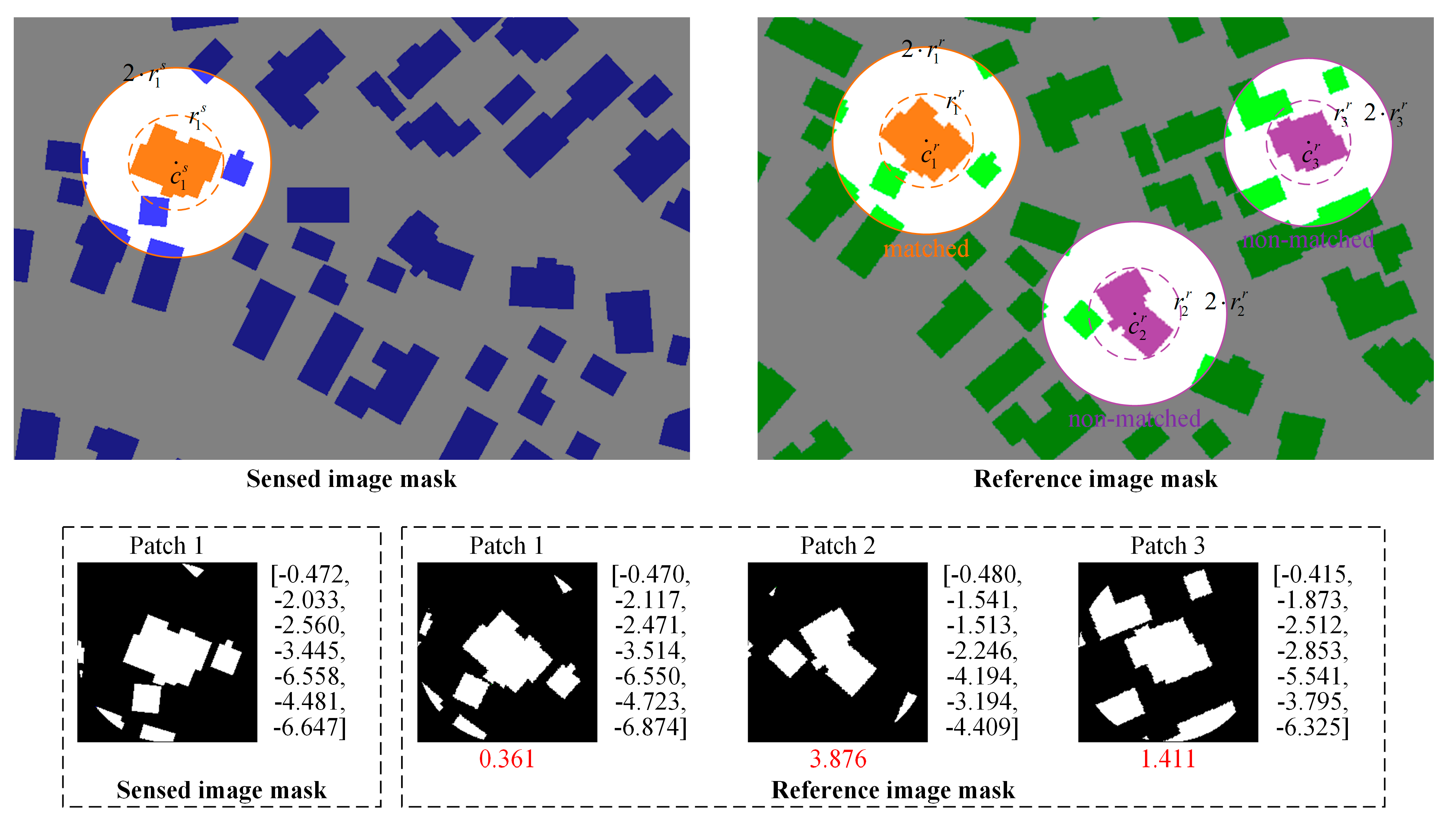
As mentioned above, we generate corresponding local areas (i.e., image block pairs) of sensed and reference images by matching instances in their segmentation masks. In order to deal with the problem of the sensed image with poor positioning accuracy, we present a strategy that does not rely on geospatial information but only exploits image processing to achieve instance matching. The concept of moments can be used for binary or gray level region description, a set of moments calculated from a digital image usually describes different types of geometric characteristic information of the global image, such as size, position, direction, shape, etc. Hu moments are highly condensed image features, which can measure the similarity of two gray-scale images and are robust to translation, rotation, and scale changes [44]. Hu moments are characterized by fast speed and a better description of shape features, but a poor description of texture features [45]. Our instance segmentation masks are binary and only contain instance shapes without texture. In addition, our instance segmentation model is dedicated to obtaining fine-grained instance boundaries. Thus, the corresponding instances have similar geometric shapes. Therefore, based on Hu moments to realize instance matching, the detailed steps are as follows.
  • For both instance segmentation masks, we use morphological operations, such as dilation followed by erosion to fill gaps and remove noise.
  • For each instance in the sensed image, we take its minimum enclosing circle (the result of instance segmentation includes the contour coordinates). The center of the circle is denoted as c i s , and the radius is denoted as r i s .
  • We take a circular patch as the local area to make it rotation invariant. The patch has c i s as its center and m r i s as its radius, where m is the expansion scale. This is done because the patch formed by the instance and its neighbors has a higher accuracy for matching than the single instance. Since we use OpenCV to calculate the Hu moments and it requires the input to be a matrix, we fill the circular patch with 0 into its smallest external square (the instances are filled with 1 and the background is 0 in our binary segmentation masks) and we can obtain the Hu moments of each instance patch in the sensed image.
  • For each instance in the reference image, the center of the minimum enclosing circle of the instance is denoted as c i r , and the radius is denoted as r i r . We use the same approach to get the Hu moments of each instance patch. Note that, since the Hu moments calculated directly have a small order of magnitude, we actually take their base 10 logarithms as the result, which is the same as in Reference [45].
  • For each Hu moments vector in the sensed image, we use brute force matching to find the vector with the smallest Euclidean distance in the reference image, thereby, achieving instance matching. In fact, this step can be implemented quickly through matrix operations. The above steps are depicted in Figure 7.
  • For each pair of matching instances, we take c i s and c i r as the centers and generate a pair of boxes of size δ × δ in the sensed and reference images, respectively. We filter out the boxes with the Intersection over Union (IoU) greater than 0.5 in the same image, which is the same as in Reference [27]. Finally, we crop the remaining pairs of boxes into the corresponding image block pairs. This step is illustrated in Figure 5.
  • We discuss the impact of the values of m and δ on performance in the subsequent experiments, and we take m as 2 and δ as 600 in this paper. Please refer to Section 4 for details.

3.3. Local Feature Matching, Outlier Removal, and Registration

Based on the generated image block pairs, the steps of outlier removal and the final registration are as follows.
  • For each image block pair, we mask out the unwanted instances and adopt a classic feature-based method (such as SIFT, etc.) to obtain the initial matching key points. The key points are matched by the Euclidean distance ratio between the nearest neighbor and the second nearest neighbor of corresponding features, and the ratio is set to 0.8, which is the same as in Reference [6]. This step is illustrated in Figure 5.
  • We eliminate the key points of mismatch through multi-constraints. First, we introduce a cross-validation strategy, which identify the mismatches based on whether the center instances of the image block pair have similar relative positions with the key points. Since many classic hand-crafted features (SIFT, SURF, ORB, etc.) are rotation invariant, we can obtain the relative positions according to the major orientations (which are included in their features) of the key points. Specifically, we denote a pair of matching key points in the sensed and reference image blocks as p i s and p i r , respectively. Taking p i s and p i r as the origins and their major orientations as the positive directions of the x-axes, we can get the locations of c i s and c i r in the corresponding coordinate systems. In fact, the coordinates of c i s and c i r are the relative position vectors of the key points and the corresponding center instances. Then, we calculate the Euclidean distance of the pair of vectors. If it is greater than the threshold t h c v , it is considered a false match and eliminated. The t h c v is set to 10 in this paper, and please refer to Section 4 for details. Note that the relative position vector does not have scale invariance. If the spatial resolutions of the sensed and reference images are different, it is necessary to scale with the ratio of the resolutions while calculating the relative position vectors. Figure 8 illustrates an example of the cross-validation in detail.
  • RANSAC is used to further eliminate false matches for a more accurate matching result. Finally, the affine matrix T is computed by the least squares algorithm.

4. Experiments and Results

In this section, we test the instance segmentation model SSFG and the instance segmentation based registration framework on large-sized, high-resolution remote sensing images, compared them with related works, and analyzed the experimental results.

4.1. Instance Segmentation for High-Resolution Remote Sensing Images

4.1.1. Datasets and Metrics

We use three datasets for experiments to test the effect of SSFG for high-resolution remote sensing image instance segmentation. First, to compare with the methods in References [28,29,30], we use the same dataset Vaihingen [46] as in their experiments to carry out the building instance segmentation experiment. Vaihingen is a public aerial image dataset with a spatial resolution of 9 cm, which is provided by the ISPRS. We follow the same data partition as in Reference [28] to divide the training set and test set. Second, we use WHU Building Dataset [26] to do the building instance segmentation experiment. We only use the aerial images in this dataset, whose number is 8189, size is 512 × 512, and the spatial resolution is 30 cm. We follow the original data partition to acquire the training, validation, and test sets. Finally, we use a self-made dataset Jilin-1-HZ to perform the pond and greenhouse instance segmentation experiments. The images in Jilin-1-HZ come from the Jilin-1 satellite image data. The original images cover 15,000 km2 on Hangzhou, China with 0.75 m spatial resolution, and images are multi-period. Expert manual annotations are provided for four classes: pond, greenhouse, tea, and rice field, while pond and greenhouse labels are used in our experiments. We crop the areas containing the instances in the original images into 10,422 tiles with a size of 896 × 896, and randomly divide 1/2, 1/6, and 1/3 of them into training, validation, and test sets, respectively.
We measure the accuracy using four different metrics, which are adopted in References [28,29,30]. Dice, mean Intersection over Union (mIoU), Weighted Coverage (WCov) [47], and Boundary F-score (BoundF) [48]. Among them, BoundF focuses more on evaluating the accuracy of boundary prediction. In addition, the experiments in this paper are all single-category, so the mIoU is actually IoU.

4.1.2. Implementation Details of the SSFG

We implement the SSFG based on the MMDetection [49], the SOLO benchmark project (https://github.com/WXinlong/SOLO, accessed date: 1 January 2021), and the SegFix benchmark project (https://github.com/openseg-group/openseg.pytorch, accessed date: 1 January 2021). We use the pretrained HRNetV2p-W40 as the backbone, which is provided by the MMDetection model zoo, and we initialize the newly added layers as in Reference [43]. The number of grids in the SOLOv2 head is set as in Reference [39]. The generation of the boundary labels and direction labels for the SegFix branch is the same as in Reference [40]. We train for 36 epochs on Vaihingen, 60 epochs on WHU Building Dataset, and 60 epochs on Jilin-1-HZ. For Vaihingen and WHU Building Dataset, the batch size is 4 and the layers of BiFPN in the SSFG is 3, as recommended in Reference [42] (input size of 512 × 512 pixels). For Jilin-1-HZ, the batch size is 2 and the layers of BiFPN is 6 (input size of 896 × 896). The SSFG are compared with DSAC [28], DarNet [29], and TDAC [30] on Vaihingen, and SiU-Net [26] on WHU Building Dataset, which are state-of-the-art high-resolution remote sensing image instance segmentation methods. In addition, we adopt three state-of-the-art benchmarks Msak RCNN [27], Yolact [50], and PointRend [51] for comparison on Jilin-1-HZ, and they are all implemented based on the MMDetection. Stochastic gradient descent (SGD) is used as an optimizer, and its weight decay and momentum are set as 0.0001 and 0.9, respectively. The initial learning rate is 0.001 and is reduced tenfold after 3/4 and 11/12 of the total epochs.

4.1.3. Results

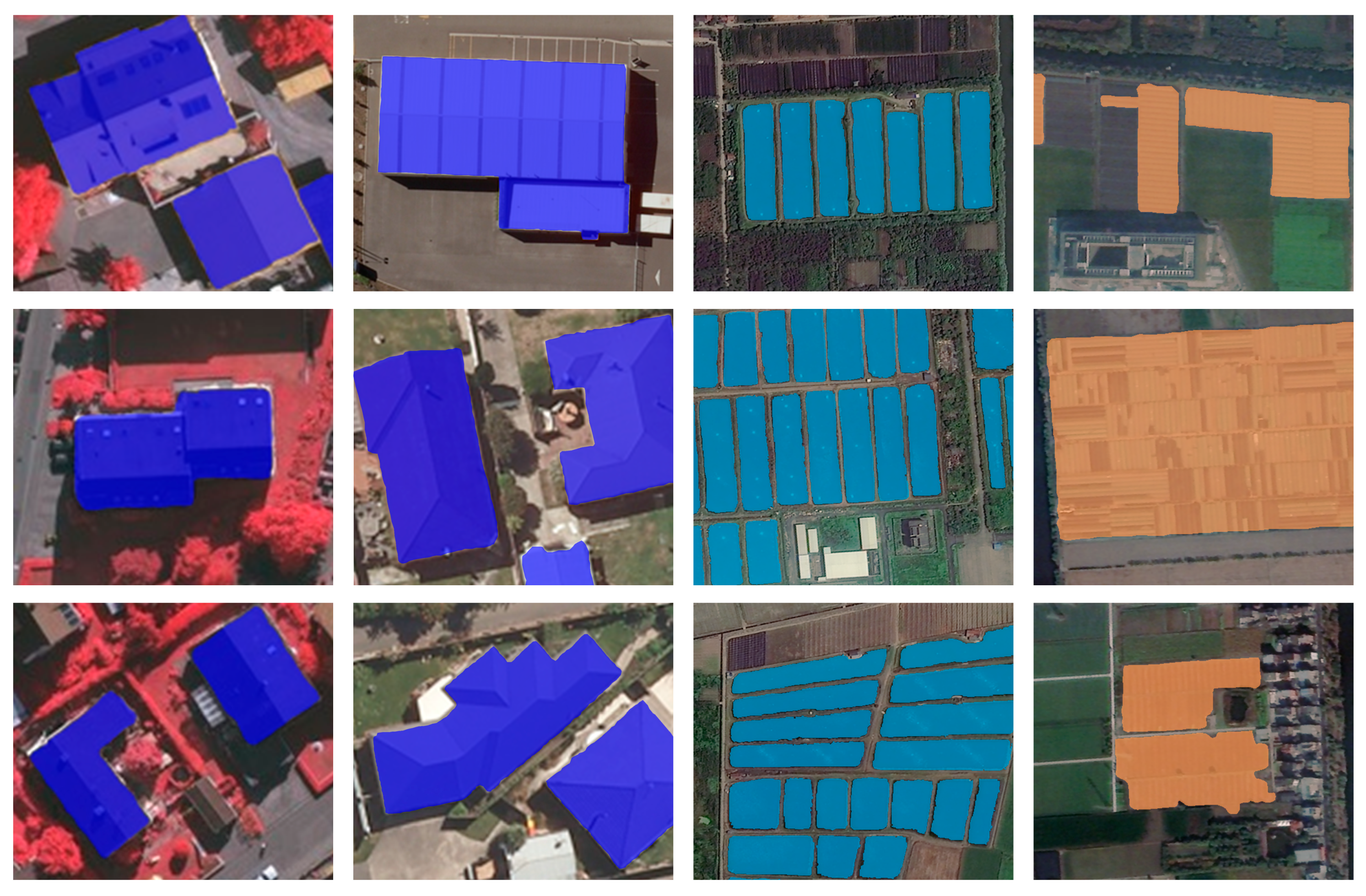
The quantitative results of the Vaihingen, WHU Building Dataset, Jilin-1-HZ Pond, and Jilin-1-HZ Greenhouse experiments are illustrated in Table 1, Table 2, Table 3 and Table 4, respectively. Meanwhile, the visualization test results are depicted in Figure 9, which intuitively confirm the fine-grained effect of the SSFG. Table 1 and Table 2 show that the SSFG achieves either superior or competitive performances to state-of-the-art methods, which are dedicated to the building instance segmentation of high-resolution remote sensing images. Table 3 and Table 4 reflects the SSFG outperforms state-of-the-art instance segmentation benchmarks on high-resolution remote sensing images. Note that the BoundF is an indicator that focuses on measuring the accuracy and fineness of the boundary as mentioned above. Our BoundF values are the best in all experiments, and is higher than the second place at about 5.4% on average. The experiments prove that the combination of high-resolution representation backbone, attention mechanism, and boundary post-processing can effectively improve the instance segmentation accuracy of high-resolution remote sensing images. Furthermore, Table 3 and Table 4 show the frames per second (FPS) of each method, and the SSFG is second only to the Yolact. Note that the SSFG uses a more complex backbone than the compared methods and adds an attention mechanism, but its speed is about twice of the Mask RCNN as well as the PointRend, which confirms the efficiency of the single-stage strategy of the SSFG.

4.2. High-Resolution Remote Sensing Image Registration

4.2.1. Test Data and Evaluation Metrics

In this section, three pairs of large high-resolution remote sensing images are tested in our experiments, where Christchurch is from WHU Building Dataset and Hangzhou-1 and Hangzhou-2 are from Jilin-1-HZ. The description of the test data is given in Table 5. For each pair, since the original images we obtained have already been registered, we select the newly shooting image for random affine transformation as the reference image, and the other as the sensed image for the experiment. We perform slightly, moderately, and heavily random affine transformations on Christchurch, Hangzhou-1, and Hangzhou-2 to simulate the high, medium, and poor positioning accuracy, respectively. For each pair, a total of 100 Ground Control Point (GCP) pairs are carefully selected from the sensed and reference images by experts, which are distributed as evenly as possible in the two images. These GCP pairs are used as the reference to test the precision of a registration method, and the precision is evaluated by the Root-Mean-Square Error (RMSE), which is defined as follows.
R M S E = 1 N i = 1 N r x i 2 + r y i 2 ,
where N is the number of matches and r x i , r y i is the residual for a certain match. In addition, we adopt the number of correct correspondences (NOCC) and ratio of correct correspondences (ROCC) to evaluate the robustness of the registration, which are the same as in Reference [4].

4.2.2. Implementation Details of the Instance Segmentation Based Registration Framework

For the Christchurch experiment, we do the building instance segmentation to generate the image block pairs. While, for Hangzhou-1 and Hangzhou-2 experiments, we do two categories of instance segmentation (pond and greenhouse). The other details of our method are the same as illustrated in Section 3. Our method is compared to state-of-the-art methods Affine-SIFT [11], SAR-SIFT [12], PSO-SIFT [13], CFOG [14], and the classic SIFT [6] on the test data. At the same time, we respectively adopt SIFT, SURF [7], and ORB [8] as the local feature matching method of our framework for the ablation study. The key points are matched by the Euclidean distance ratio between the nearest neighbor and the second nearest neighbor of corresponding features, and the ratios for SIFT, Affine-SIFT, SAR-SIFT, and PSO-SIFT are 0.8, 0.8, 0.9, and 0.9 (which are the recommended values in their papers), respectively. We implement SIFT, SAR-SIFT, and PSO-SIFT based on the ‘Image-Registration’ project (https://github.com/ZeLianWen/Image-Registration, accessed date: 1 January 2021), implement Affine-SIFT based on its official demo (http://www.cmap.polytechnique.fr/~yu/research/ASIFT/demo.html, accessed date: 1 January 2021), and implement CFOG based on its official demo (https://github.com/yeyuanxin110/ CFOG, accessed date: 1 January 2021). For Affine-SIFT, SAR-SIFT, PSO-SIFT, and SIFT, we load the sensed and reference images in grayscale and divide them into corresponding image block pairs to perform registration, and the image block pairs are acquired by a seamlessly sliding window. The window size is set to 600 × 600 pixels so as to be the same as the input size of ours.

4.2.3. Results

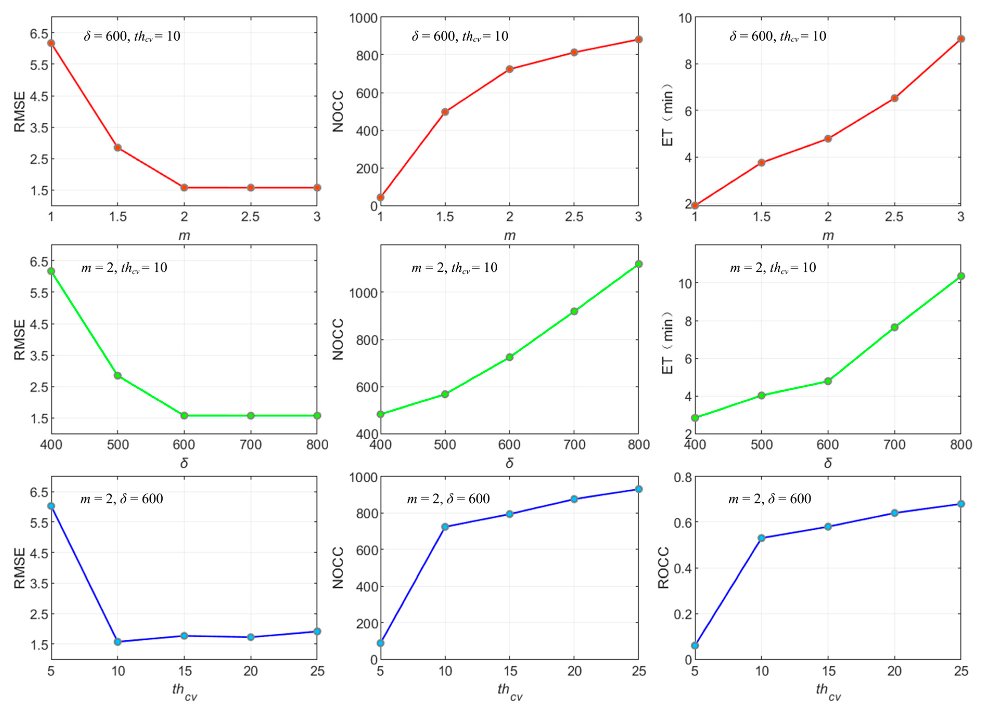
We study the influence of the values of the three parameters m , δ , and t h c v in our framework for the registration result. m determines the radii of the circular patches for the instance matching, which affects the accuracy of the instance matching. δ is the size of the local areas, which affects the number and accuracy of the initial matching key points. t h c v is the threshold of the Euclidean distance for the outlier removal, which affects the number and accuracy of the final matching key points. We control variables for experiments and the results are shown in Figure 10. The ET in the figure refers to the execution time, and the unit is minutes. According to the results and comprehensively considering the accuracy (RMSE), robustness (NOCC and ROCC), and efficiency (ET), we choose that m = 2 , δ = 600 , and t h c v = 10 as a set of optimal parameters, which is used in the follow-up experiments.
The quantitative results of the registration experiments are shown in Table 6, Table 7 and Table 8. The following points can be drawn from the analysis of the results. First, in the Christchurch and Hangzhou-1 experiments, the RMSE of our method are the best. That is, our registration accuracy for large-sized, high-resolution remote sensing images surpasses state-of-the-art feature-based methods Affine-SIFT, SAR-SIFT, PSO-SIFT, and CFOG, as well as the classic SIFT. In addition, the robustness indicator ROCC of our method ranks second (second only to CFOG). The RMSE and ROCC results confirm the effectiveness of the proposed framework, including the use of instance segmentation results as the deep features, as well as the instance matching and outlier removal strategies. Furthermore, we shield the ground objects that may affect the registration accuracy during the local feature matching, and we believe it is one of the reasons for our accuracy advantage.
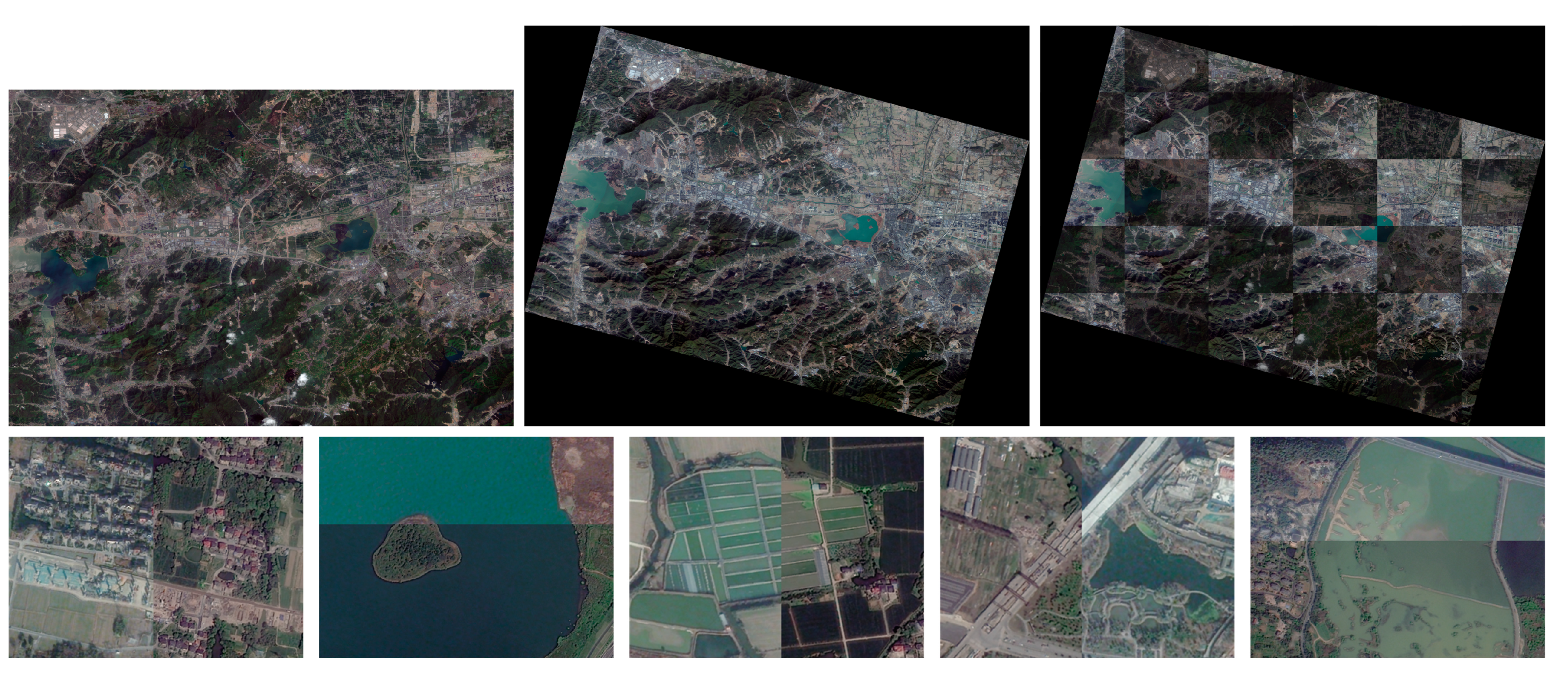
Second, in the Hangzhou-2 experiment, we simulate a scene of the sensed image with poor positioning accuracy (the PE is about 1.2 km). At this time, as analyzed in Section 2, the related works rely on the geospatial information to obtain the corresponding sensed and reference image block pairs, and there are no actual overlapping areas between them. Thus, the subsequent registration steps are wasted while resulting in the failure of the task. In this case, the applicability, accuracy, and efficiency of our method are not affected at all. That is, our method effectively copes with the circumstance of the sensed image with poor positioning accuracy.
Third, ET in the table represents the execution time (in minutes), which is the same as in Figure 10. Our method achieves the highest registration efficiency in the three experiments. Note here that our ET does not include the time of performing the instance segmentation. This is because the time largely depends on the number and performance of the GPU devices, and the related works do not involve similar GPU operations. Therefore, we believe that it is not objective and comparable to limit the number and model of GPUs to calculate the time. In fact, our instance segmentation model SSFG is efficient. Taking the Christchurch experiment as an example, we use four NVIDIA TITAN RTX GPUs in parallel operation, and the execution time of instance segmentation is less than 10 s. Even if we add this to our ET, it is still the fastest. Our efficiency advantage is mainly due to the fact that we only select the matching local areas in the images to perform the feature-based registration process, so the overall input and calculation amount are far less than related methods.
Finally, the experiment reflects that, for large-sized, high-resolution remote sensing images, the registration accuracy is not positively correlated with the amount of input information and the number of correct matching key points. In the Christchurch and Hangzhou-1 experiments, our NOCC is the least (less than 1/10 of the maximum), but our accuracy (RMSE) is the highest. Related works use the entire content of the images as an undifferentiated registration element, which leads to a surplus of input information, and the redundant information may not necessarily improve accuracy but may be counterproductive. For large-sized, high-resolution remote sensing images, we believe that it is more reasonable and efficient to perform registration using only valid local features, which can provide gains for the registration work.
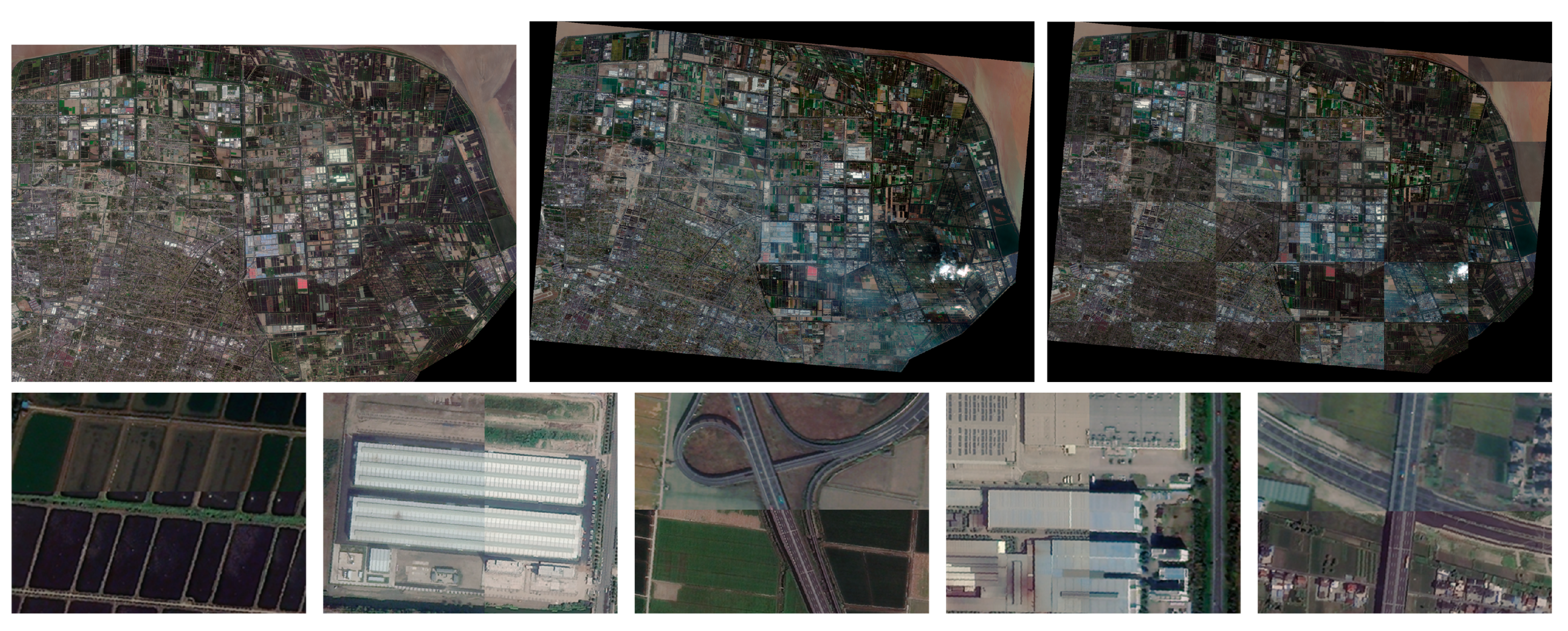
Figure 11, Figure 12 and Figure 13 are the visualization results of our method on the experiments. In each picture, from left to right in the first row is the sensed image, the reference image, and the registration result on the checkerboard mosaiced image, respectively. The second row is the display of some partial details. The satisfactory effects of our method are confirmed in the figures.

5. Conclusions

We focus on the specific scene of large-sized, high-resolution remote sensing image registration, and consider the practical application difficulties, which have not been explored by related works. For this purpose, we propose a novel automatic registration framework based on instance segmentation. The proposal makes full use of the CNN to extract deep features, which overcomes the limitations of hand-crafted features for remote sensing images. In addition, the approach achieves local area matching through image processing without relying on the geospatial information, thus, effectively coping with the problem of poor positioning accuracy. Based on the instance segmentation results and the introduced outlier removal strategy, the accuracy of local feature matching as well as the final registration is improved. Furthermore, the method only uses local features as registration elements, so it is very efficient. The above advantages have been confirmed in substantial experiments. In follow-up research, we will explore the feasibility of replacing the local feature matching method from hand-crafted features to deep features.

Author Contributions

Conceptualization, J.L. and T.L. Data curation, Z.L. and J.M. Formal analysis, Z.L. and J.M. Funding acquisition, H.J. and R.Z. Investigation, Z.L. and J.M. Methodology, J.L. and T.L. Project administration, H.J. and R.Z. Resources, Z.L. and J.M. Software, J.L. and T.L. Supervision, H.J. and R.Z. Validation, J.L. and T.L. Visualization, J.L. and T.L. Writing—original draft, J.L. and T.L. Writing—review & editing, J.L. and T.L. All authors have read and agreed to the published version of the manuscript.

Funding

This research was funded by the National Key Research and Development Program of China, grant number SQ2020YFA070264, and Major Science and Technology Projects of Jilin Province, grant number 20200503002SF, and Major Science and Technology Project of Hainan Province, grant number ZDKJ2019007.

Institutional Review Board Statement

Not applicable.

Informed Consent Statement

Not applicable.

Data Availability Statement

The Vaihingen dataset is available at http://www2.isprs.org/commissions/comm3/wg4/benchmark/semantic-labeling.html, and WHU Building Dataset is available at http://study.rsgis.whu.edu.cn/pages/download/.

Acknowledgments

Special thanks to the Jilin-1 high-resolution satellite image data, and Yifei Li, Liying Zhang, and Peng Huang for their works on data production and annotation. We also thank Fang Wan, Peng Zhang, Wentao Li, and Qing Lu for their help on the infrastructure and discussion. We thank the open-source community for the contributions.

Conflicts of Interest

The authors declare no conflict of interest.

References

  1. Zitova, B.; Flusser, J. Image registration methods: A survey. Image Vis. Comput. 2003, 21, 977–1000. [Google Scholar] [CrossRef] [Green Version]
  2. Brown, L.G. A survey of image registration techniques. ACM Comput. Surv. 1992, 24, 325–376. [Google Scholar] [CrossRef]
  3. Le Moigne, J. Introduction to remote sensing image registration. In Proceedings of the IEEE International Geoscience and Remote Sensing Symposium (IGARSS), Fort Worth, TX, USA, 23–28 July 2017; pp. 2565–2568. [Google Scholar]
  4. Ma, W.; Zhang, J.; Wu, Y.; Jiao, L.; Zhu, H.; Zhao, W. A novel two-step registration method for remote sensing images based on deep and local features. IEEE Trans. Geosci. Remote Sens. 2019, 57, 4834–4843. [Google Scholar] [CrossRef]
  5. Zhu, H.; Jiao, L.; Ma, W.; Liu, F.; Zhao, W. A novel neural network for remote sensing image matching. IEEE Trans. Neural Netw. Learn. Syst. 2019, 30, 2853–2865. [Google Scholar] [CrossRef]
  6. Lowe, D.G. Distinctive image features from scale-invariant keypoints. Int. J. Comput. Vis. 2004, 60, 91–110. [Google Scholar] [CrossRef]
  7. Bay, H.; Tuytelaars, T.; Van Gool, L. Surf: Speeded up robust features. In Proceedings of the European Conference on Computer Vision, Graz, Austria, 7–13 May 2006; pp. 404–417. [Google Scholar]
  8. Rublee, E.; Rabaud, V.; Konolige, K.; Bradski, G. ORB: An efficient alternative to SIFT or SURF. In Proceedings of the IEEE International Conference on Computer Vision, Barcelona, Spain, 6–13 November 2011; pp. 2564–2571. [Google Scholar]
  9. Alcantarilla, P.F.; Solutions, T. Fast explicit diffusion for accelerated features in nonlinear scale spaces. IEEE Trans. Patt. Anal. Mach. Intell. 2011, 34, 1281–1298. [Google Scholar]
  10. Fischler, M.A.; Bolles, R.C. Random sample consensus: A paradigm for model fitting with applications to image analysis and automated cartography. Commun. ACM 1981, 24, 381–395. [Google Scholar] [CrossRef]
  11. Morel, J.M.; Yu, G. ASIFT: A new framework for fully affine invariant image comparison. SIAM J. Imaging Sci. 2009, 2, 438–469. [Google Scholar] [CrossRef]
  12. Dellinger, F.; Delon, J.; Gousseau, Y.; Michel, J.; Tupin, F. SAR-SIFT: A SIFT-like algorithm for SAR images. IEEE Trans. Geosci. Remote Sens. 2014, 53, 453–466. [Google Scholar] [CrossRef] [Green Version]
  13. Ma, W.; Wen, Z.; Wu, Y.; Jiao, L.; Gong, M.; Zheng, Y.; Liu, L. Remote sensing image registration with modified SIFT and enhanced feature matching. IEEE Geosci. Remote Sens. Lett. 2016, 14, 3–7. [Google Scholar] [CrossRef]
  14. Ye, Y.; Bruzzone, L.; Shan, J.; Bovolo, F.; Qing, Z. Fast and robust matching for multimodal remote sensing image registration. IEEE Trans. Geosci. Remote Sens. 2019, 57, 9059–9070. [Google Scholar] [CrossRef] [Green Version]
  15. Huo, C.; Pan, C.; Huo, L.; Zhou, Z. Multilevel SIFT matching for large-size VHR image registration. IEEE Geosci. Rem. Sens. Lett. 2011, 9, 171–175. [Google Scholar] [CrossRef]
  16. Ma, J.; Chan, J.C.W.; Canters, F. Fully automatic subpixel image registration of multiangle CHRIS/Proba data. IEEE Trans. Geosci. Remote Sens. 2010, 48, 2829–2839. [Google Scholar]
  17. Sedaghat, A.; Mokhtarzade, M.; Ebadi, H. Uniform robust scale-invariant feature matching for optical remote sensing images. IEEE Trans. Geosci. Remote Sens. 2011, 49, 4516–4527. [Google Scholar] [CrossRef]
  18. Goncalves, H.; Corte-Real, L.; Goncalves, J.A. Automatic image registration through image segmentation and SIFT. IEEE Trans. Geosci. Remote Sens. 2011, 49, 2589–2600. [Google Scholar] [CrossRef] [Green Version]
  19. Gong, M.; Zhao, S.; Jiao, L.; Tian, D.; Wang, S. A novel coarse-to-fine scheme for automatic image registration based on SIFT and mutual information. IEEE Trans. Geosci. Remote Sens. 2013, 52, 4328–4338. [Google Scholar] [CrossRef]
  20. Ye, Y.; Shan, J. A local descriptor based registration method for multispectral remote sensing images with non-linear intensity differences. ISPRS J. Photogramm. Remote Sens. 2014, 90, 83–95. [Google Scholar] [CrossRef]
  21. Kupfer, B.; Netanyahu, N.S.; Shimshoni, I. An efficient SIFT-based mode-seeking algorithm for sub-pixel registration of remotely sensed images. IEEE Geosci. Remote Sens. Lett. 2014, 12, 379–383. [Google Scholar] [CrossRef]
  22. Wu, Y.; Ma, W.; Gong, M.; Su, L.; Jiao, L. A novel point-matching algorithm based on fast sample consensus for image registration. IEEE Geosci. Remote Sens. Lett. 2014, 12, 43–47. [Google Scholar] [CrossRef]
  23. Ye, Y.; Shen, L. Hopc: A novel similarity metric based on geometric structural properties for multi-modal remote sensing image matching. ISPRS Ann. Photogramm. Remote Sens. Spat. Inf. Sci. 2016, 3, 9. [Google Scholar] [CrossRef] [Green Version]
  24. Ye, Y.; Shan, J.; Bruzzone, L.; Shen, L. Robust registration of multimodal remote sensing images based on structural similarity. IEEE Trans. Geosci. Remote Sens. 2017, 55, 2941–2958. [Google Scholar] [CrossRef]
  25. Wang, S.; Quan, D.; Liang, X.; Ning, M.; Guo, Y.; Jiao, L. A deep learning framework for remote sensing image registration. ISPRS J. Photogramm. Remote Sens. 2018, 145, 148–164. [Google Scholar] [CrossRef]
  26. Ji, S.; Wei, S.; Lu, M. Fully convolutional networks for multisource building extraction from an open aerial and satellite imagery data set. IEEE Trans. Geosci. Remote Sens. 2018, 57, 574–586. [Google Scholar] [CrossRef]
  27. He, K.; Gkioxari, G.; Dollár, P.; Girshick, R. Mask r-cnn. In Proceedings of the IEEE International Conference on Computer Vision, Venice, Italy, 22–29 October 2017; pp. 2961–2969. [Google Scholar]
  28. Marcos, D.; Tuia, D.; Kellenberger, B.; Zhang, L.; Bai, M.; Liao, R.; Urtasun, R. Learning deep structured active contours end-to-end. In Proceedings of the IEEE Conference on Computer Vision and Pattern Recognition, Salt Lake City, UT, USA, 18–22 June 2018; pp. 8877–8885. [Google Scholar]
  29. Cheng, D.; Liao, R.; Fidler, S.; Urtasun, R. Darnet: Deep active ray network for building segmentation. In Proceedings of the IEEE/CVF Conference on Computer Vision and Pattern Recognition, Long Beach, CA, USA, 16–20 June 2019; pp. 7431–7439. [Google Scholar]
  30. Hatamizadeh, A.; Sengupta, D.; Terzopoulos, D. End-to-end trainable deep active contour models for automated image segmentation: Delineating buildings in aerial imagery. In Proceedings of the European Conference on Computer Vision, Glasgow, UK, 23–28 August 2020; pp. 730–746. [Google Scholar]
  31. Hamaguchi, R.; Fujita, A.; Nemoto, K.; Imaizumi, T.; Hikosaka, S. Effective use of dilated convolutions for segmenting small object instances in remote sensing imagery. In Proceedings of the IEEE Winter Conference on Applications of Computer Vision (WACV), Lake Tahoe, CA, USA, 12–15 March 2018; pp. 1442–1450. [Google Scholar]
  32. Mou, L.; Zhu, X.X. Vehicle instance segmentation from aerial image and video using a multitask learning residual fully convolutional network. IEEE Trans. Geosci. Remote Sens. 2018, 56, 6699–6711. [Google Scholar] [CrossRef] [Green Version]
  33. Feng, Y.; Diao, W.; Zhang, Y.; Li, H.; Chang, Z.; Yan, M.; Sun, X.; Gao, X. Ship Instance segmentation from remote sensing images using sequence local context module. In Proceedings of the 2019 IEEE International Geoscience and Remote Sensing Symposium, Yokohama, Japan, 28 July–2 August 2019; pp. 1025–1028. [Google Scholar]
  34. Lu, J.; Jia, H.; Gao, F.; Li, W.; Lu, Q. Reconstruction of digital surface model of single-view remote sensing image by semantic segmentation network. J. Electr. Inf. Technol. 2021, 43, 974–981. [Google Scholar]
  35. Li, Z.; Zhu, R.; Ma, J.; Meng, X.; Wang, D.; Liu, S. Airport detection method combined with continuous learning of residual-based network on remote sensing image. Acta Opt. Sin. 2020, 40, 1628005. [Google Scholar]
  36. Zhu, R.; Ma, J.; Li, Z.; Wang, D.; An, Y.; Zhong, X.; Gao, F.; Meng, X. Domestic multispectral image classification based on multilayer perception convolutional neural network. Acta Opt. Sin. 2020, 40, 1528003. [Google Scholar]
  37. Lu, J.; Li, T.; Ma, J.; Li, Z.; Jia, H. SAR: Single-stage anchor-free rotating object detection. IEEE Access 2020, 8, 205902–205912. [Google Scholar] [CrossRef]
  38. Wang, X.; Kong, T.; Shen, C.; Jiang, Y.; Li, L. Solo: Segmenting objects by locations. In Proceedings of the European Conference on Computer Vision, Glasgow, UK, 23–28 August 2020; pp. 649–665. [Google Scholar]
  39. Wang, X.; Zhang, R.; Kong, T.; Li, L.; Shen, C. SOLOv2: Dynamic and fast instance segmentation. Adv. Neural Inf. Process. Syst. 2020, 33, 1–17. [Google Scholar]
  40. Yuan, Y.; Xie, J.; Chen, X.; Wang, J. Segfix: Model-agnostic boundary refinement for segmentation. In Proceedings of the European Conference on Computer Vision, Glasgow, UK, 23–28 August 2020; pp. 489–506. [Google Scholar]
  41. Sun, K.; Zhao, Y.; Jiang, B.; Cheng, T.; Xiao, B.; Liu, D.; Mu, Y.; Wang, X.; Liu, W.; Wang, J. High-Resolution Representations for Labeling Pixels and Regions. 2019. Available online: https://arxiv.org/abs/1904.04514 (accessed on 9 April 2019).
  42. Tan, M.; Pang, R.; Le, Q.V. Efficientdet: Scalable and efficient object detection. In Proceedings of the IEEE/CVF Conference on Computer Vision and Pattern Recognition, Seattle, WA, USA, 14–19 June 2020; pp. 10781–10790. [Google Scholar]
  43. Lin, T.Y.; Goyal, P.; Girshick, R.; He, K.; Dollár, P. Focal loss for dense object detection. In Proceedings of the IEEE International Conference on Computer Vision, Venice, Italy, 22–29 October 2017; pp. 2980–2988. [Google Scholar]
  44. Hu, M.K. Visual pattern recognition by moment invariants. IRE Trans. Inf. Theory 1962, 8, 179–187. [Google Scholar]
  45. Huang, Z.; Leng, J. Analysis of Hu’s moment invariants on image scaling and rotation. In Proceedings of the IEEE 2010 2nd International Conference on Computer Engineering and Technology, Chengdu, China, 16–18 April 2010; pp. 476–480. [Google Scholar]
  46. Cramer, M. The DGPF-test on digital airborne camera evaluation overview and test design. PFG Photogramm. Fernerkund. Geoinf. 2010, 2, 73–82. [Google Scholar] [CrossRef] [PubMed]
  47. Silberman, N.; Sontag, D.; Fergus, R. Instance segmentation of indoor scenes using a coverage loss. In Proceedings of the European Conference on Computer Vision, Zurich, Switzerland, 6–12 September 2014; pp. 616–631. [Google Scholar]
  48. Perazzi, F.; Pont-Tuset, J.; McWilliams, B.; Van Gool, L.; Gross, M.; Sorkine-Hornung, A. A benchmark dataset and evaluation methodology for video object segmentation. In Proceedings of the IEEE Conference on Computer Vision and Pattern Recognition, Las Vegas, NV, USA, 26 June–1 July 2016; pp. 724–732. [Google Scholar]
  49. Chen, K.; Wang, J.; Pang, J.; Cao, Y.; Xiong, Y.; Li, X.; Sun, S.; Feng, W.; Liu, Z.; Xu, J.; et al. MMDetection: Open Mmlab Detection toolbox and Benchmark. 2019. Available online: https://arxiv.org/abs/1906.07155 (accessed on 17 June 2019).
  50. Bolya, D.; Zhou, C.; Xiao, F.; Lee, Y.J. Yolact: Real-time instance segmentation. In Proceedings of the IEEE/CVF International Conference on Computer Vision, Seoul, Korea, 27 October–2 November 2019; pp. 9157–9166. [Google Scholar]
  51. Kirillov, A.; Wu, Y.; He, K.; Girshick, R. Pointrend: Image segmentation as rendering. In Proceedings of the IEEE/CVF Conference on Computer Vision and Pattern Recognition, Seattle, WA, USA, 14–19 June 2020; pp. 9799–9808. [Google Scholar]
Figure 1. The problem of non-correspondence between the (a) sensed image with poor positioning accuracy and (b) the reference image.
Remotesensing 13 01657 g001
Figure 2. The registration result of the entire large-sized, high-resolution (a) sensed image and (b) reference image.
Remotesensing 13 01657 g002
Figure 3. The (a) correct matches on the ground and the (b) mismatches on the buildings.
Remotesensing 13 01657 g003
Figure 4. The detected key points on (a) summer greenhouses, (b) winter greenhouses, (c) summer ponds, and (d) winter ponds.
Remotesensing 13 01657 g004
Figure 5. The proposed instance segmentation based framework for large-sized, high-resolution, remote sensing image registration.
Remotesensing 13 01657 g005
Figure 6. The structure of our single-stage, fine-grained, instance segmentation network for high-resolution remote sensing images. The input size in this paper is 896 × 896 and note that the BiFPN requires the input size to be a multiple of 128 pixels. P2-P6 indicate the HRNetV2p backbone output layers. In the instance segmentation head of each BiFPN output layer, the three branches represent the classification branch, kernel branch, and feature branch, respectively, which is the same as in SOLOv2. ‘Align’ means the adaptive-pooling, which is the same as in Reference [38]. C refers to the number of the instance categories. S × S refers to the number of grids in SOLOv2, and s refers to the scale of the input size while 1/4s is 228 × 228 in this paper. In the feature branch, each BiFPN output layer is up-sampled by convolutions and bilinear interpolations until it reaches 1/4 scale, and indicates the element-wise summation of them to acquire the unified feature. denotes the dynamic convolution operation, which is the same as in Reference [39]. denotes the fusion of the boundary map and the direction map and ‘Refinement’ denotes the post-processing of the coarse mask, which is the same as in Reference [40].
Remotesensing 13 01657 g006
Figure 7. The illustration of instance matching. Note that our instance segmentation masks are binary, and, here, we painted them in color to make it easier to understand. The vector on the right side of each patch is its Hu moments (take their base 10 logarithms). The red number below each reference patch represents the Euclidean distance between its Hu moments vector and the Hu moments vector of the sensed patch. The figure shows the rotation invariance of the circular patch and the effectiveness of the matching approach.
Remotesensing 13 01657 g007
Figure 8. Illustration of the cross-validation. p 1 s and p 1 r are a pair of matching key points given by SIFT, as well as p 2 s and p 2 r . The dashed arrow indicates the SIFT major orientation of each key point, that is, the positive direction of the x-axis of its coordinate system. Each dashed line without an arrow indicates the positive direction of the y-axis (note that the original positive direction of the y-axis in the image coordinate system is downward). c 1 s and c 1 r denote the centers of the minimum enclosing circles of the center instances. The solid arrow indicates the relative position vector of each key point. In this example, p 1 s c 1 s is (46.965, 110.409), and p 1 r c 1 r is (260.657, 9.204). Their Euclidean distance is 236.446. p 2 s c 1 s is (158.180, 99.205), and p 2 r c 1 r is (160.201, 96.003). Their Euclidean distance is 3.787. Therefore, p 1 s and p 1 r are key points of mismatch and eliminated. The process only involves a basic analytical geometry method, so we do not elaborate on it here.
Remotesensing 13 01657 g008
Figure 9. The SSFG instance segmentation test results on high-resolution remote sensing images. The four columns from left to right are: the building instance segmentation on Vaihingen, the building instance segmentation on WHU Building Dataset, the pond instance segmentation on Jilin-1-HZ, and the greenhouse instance segmentation on Jilin-1-HZ. We set the classification score threshold as 0.6.
Remotesensing 13 01657 g009
Figure 10. The influence of the values of m , δ , and t h c v in our framework for the registration result.
Remotesensing 13 01657 g010
Figure 11. Visualized result of our registration method on Christchurch.
Remotesensing 13 01657 g011
Figure 12. Visualized result of our registration method on Hangzhou-1.
Remotesensing 13 01657 g012
Figure 13. Visualized result of our registration method on Hangzhou-2.
Remotesensing 13 01657 g013
Table 1. Comparison with related works on the Vaihingen dataset.
MethodVaihingen
ModelBackboneDicemIoUWCovBoundF
DSAC [28]DSAC-71.1070.7036.40
DarNet [29]DarNet93.6688.2088.1075.90
TDAC [30]TDAC94.2689.1690.5478.12
SSFG (ours)HRNetV2p-W4094.7988.5190.2681.54
Table 2. Comparison with related work on WHU building dataset.
MethodWHU Building Dataset
ModelBackboneDicemIoUWCovBoundF
SiU-Net [26]U-Net-88.40--
SSFG (ours)HRNetV2p-W4093.8789.1889.9380.02
Table 3. Comparison with related works on Jilin-1-HZ pond dataset.
MethodJilin-1-HZ Pond
ModelBackboneDicemIoUWCovBoundFFPS
Yolact [50]ResNet10178.1572.0673.1139.4529.1
Mask RCNN [27]ResNet10186.7077.3682.5556.8010.4
PointRend [51]ResNet10189.3182.1385.0478.608.9
SSFG (ours)HRNetV2p-W4094.8890.6892.5483.1020.3
Table 4. Comparison with related works on Jilin-1-HZ greenhouse dataset.
MethodJilin-1-HZ Greenhouse
ModelBackboneDicemIoUWCovBoundFFPS
Yolact [50]ResNet10170.8865.4068.2137.2829.6
Mask RCNN [27]ResNet10179.5167.0377.0245.259.7
PointRend [51]ResNet10186.5280.9083.2971.459.0
SSFG (ours)HRNetV2p-W4090.1284.3985.8779.7019.5
Table 5. Test data description.
ImagePixel SizeTimeSensorResolutionInstancePE 1
ChristchurchSensed32,507 × 15,354Apr 2012Aerial0.3 mBuilding22.3 m
New ZealandReference32,771 × 15,9202016
Hangzhou-1,
China
Sensed36,004 × 24,002Aug 2020Jilin-1 Satellites0.75 mPond,
greenhouse
110.5 m
Reference37,960 × 27,050Jan 2021
Hangzhou-2,
China
Sensed36,003 × 24,002Aug 2020Jilin-1 Satellites0.75 mPond,
greenhouse
1204.1 m
Reference40,989 × 32,504Jan 2021
1 PE denotes the Positioning Error of the sensed image relative to the reference image, which is the average positioning error of the GCP pairs.
Table 6. Comparison with related works on the test data Christchurch.
MethodChristchurch
RMSENOCCROCCET (min)
SIFT [6]1.650444190.399.48
Affine-SIFT [11]6.248585060.3227.19
SAR-SIFT [12]9.831630810.4062.52
PSO-SIFT [13]1.600221650.3146.31
CFOG [14]2.310613030.693.60
ours + SIFT1.57107240.534.78
ours + SURF2.04604910.413.86
ours + ORB2.51733340.323.13
Table 7. Comparison with related works on the test data Hangzhou-1.
MethodHangzhou-1
RMSENOCCROCCET (min)
SIFT [6]4.383220790.3415.11
Affine-SIFT [11]9.258146080.3239.03
SAR-SIFT [12]14.197017130.3087.50
PSO-SIFT [13]2.417510840.4865.85
CFOG [14]2.71038550.604.05
ours + SIFT2.19884520.514.46
ours + SURF2.85812070.353.52
ours + ORB3.1062890.182.81
Table 8. Comparison with related works on the test data Hangzhou-2.
MethodHangzhou-2
RMSENOCCROCCET (min)
SIFT [6]***18.24
Affine-SIFT [11]***44.28
SAR-SIFT [12]***92.78
PSO-SIFT [13]***56.15
CFOG [14]***4.59
ours + SIFT2.86355270.454.92
ours + SURF4.06263310.293.79
ours + ORB4.41751180.143.11
* indicates that the registration has failed (RMSE > 50).
Publisher’s Note: MDPI stays neutral with regard to jurisdictional claims in published maps and institutional affiliations.