Abstract
Increasing attention has been placed on the agroecological impact of applying exogenous organic matter (EOM) amendments, such as green waste compost (GWC) and livestock manure, to agricultural landscapes. However, monitoring the frequency and locality of this practice poses a major challenge, as these events are typically unreported. The purpose of this study is to evaluate the utility of Sentinel-2 imagery for the detection of EOM amendments. Specifically, we investigated the spectral shift resulting from GWC and manure application at two spatial scales, satellite and proximal. At the satellite scale, multispectral Sentinel-2 image pairs were analyzed before and after EOM application to six cultivated fields in the Versailles Plain, France. At the proximal scale, multi-temporal spectral field measurements were taken of experimental plots consisting of 14 total treatments: EOM variety, amendment quantity (15, 30 and 60 t.ha−1) and tillage. The Sentinel-2 images showed significant spectral differences before and after EOM application. Exogenous Organic Matter Indices (EOMI) were developed and analyzed for separative performance. The best performing index was EOMI2, using the B4 and B12 Sentinel-2 spectral bands. At the proximal scale, simulated Sentinel-2 reflectance spectra, which were created using field measurements, successfully monitored all EOM treatments for three days, except for the buried green waste compost at a rate of 15 t.ha−1.
1. Introduction
The application of exogenous organic matter (EOM), such as compost and manure, to agricultural fields is a widespread practice with the objective of increasing soil fertility. Farmers use EOMs primarily to add macronutrients (nitrogen, phosphate and potassium) to their fields for crop production (fertilizing EOMs) and also to increase organic carbon content of their soils (amending EOMs) [1]. The increase of soil organic carbon (SOC) content favors soil biology and improves soil physical properties, such as aggregate stability [2]. In addition, soil organic carbon storage resulting from EOM application offers a source of greenhouses gas mitigation [3]. Soil organic carbon storage has been identified as one of the most prominent challenges of soil science in the 2020s [4] and the advancement of agricultural practices that favor SOC storage, e.g., EOM application, have been of particular focus, e.g., the 4‰ initiative [5,6].
In France, almost all EOMs which come from agriculture are spread [7], but only 14.5% of the household and similar waste and 35% of the industrial organic waste are spread [8], thus representing large potential sources of organic matter for soils. However, the practice of applying EOMs is largely undocumented, meaning little is known about the spatial allocation and frequency of amendment applications. This information is necessary to improve the understanding of agronomic and ecological impacts, such as yield estimation, soil carbon storage estimation [9] and pollution (e.g., nitrate leaching, ammonia volatilization) [10] at the landscape scale. The current method of monitoring EOM amendments is to survey farmers, which is time-consuming. In contrast, remote sensing technology offers the potential to efficiently monitor agricultural landscapes. To our knowledge, no preceding studies have addressed the detection of EOM from satellite imagery or proximal field sensors. The few studies that have examined the spectral behavior of EOMs were carried out in lab conditions, either on grape marc compost and liquid cattle manure compost [11], or hog manure [12]. Despite this knowledge gap, the spectral behavior of other organic soil compounds—crop residues and soil organic matter (SOM)—are well-studied and provide a theoretical basis for our investigation.
EOMs contain organic compounds, such as plant-derived structural compounds, humic acids and fatty acids, which can also be found in SOC and crop residues [13,14,15,16]. Moreover, SOC and EOM both produce low reflectance in the visible spectrum [17,18,19]. SOC content is a measurement of the organic compounds contained in the soil in a wide range of chemical forms: carbohydrates, polysacharrides, protein and protein-derived compounds, lipids, phenols, humic and fulvic acids, having spectral trends in the visible, NIR and SWIR regions that can be explained by combination and vibration modes of organic functional groups [17,20]. While SOC content can be predicted from bare soil surface, notably from Sentinel-2 multispectral satellite images [21,22,23,24,25,26,27], the performance of such prediction is degraded by the presence of crop residues [22,23], a form of organic matter left in the field to decompose. Crop residues are composed of insoluble carbon compound such as cellulose, hemicellulose and lignin. Some indices have been used to detect crop residues using the broader wavelength bands of the Landsat Thematic Mapper, such as “Normalized Difference Index 5” (NDI5) and “Normalized Difference Index 7” (NDI7) [28], which utilize normalized differences between the SWIR and the near infrared (NIR) spectral regions; Normalized Difference Senescent Vegetation Index (NDSVI) [29] and Normalized Difference Residue Index (NDRI) [30], both utilizing normalized differences between the SWIR and the red spectral regions; and, finally, the “Normalized Difference Tillage index” (NDTI) [31], which utilizes normalized differences between the SWIR bands. Renamed the “Normalized Burn ratio 2” (NBR2), the NDTI was adapted to Landsat8 bands [32], then used for Sentinel-2 [23,26] in order to characterize the presence of crop residues on surface and assess its influence on soil organic carbon.
Due to the similarity in chemical composition between EOM, SOC and crop residues, these spectral indices were evaluated for the detection of EOM application, in addition to the development of new indices. The detection of EOM spreading events could also be useful to determine their possible influence on the SOC prediction. However, this EOM monitoring requires high revisit time because EOM are often buried after few days and may decompose rapidly. In connection with the need to target very specific and one-shot dates of amendment applications, this study will rely on the Sentinel-2 satellite time series with a medium spatial resolution (10–20 m) and with revisit frequencies of less than five days. The purpose of this study is to determine the potential of Sentinel-2 for the detection of EOM application events and, specifically, to discern which spectral bands and indices are the most effective for this purpose. Thus, this study was conducted at two different scales: firstly, using Sentinel-2 satellites to test if EOM amending practices can be detected and secondly, using field spectral measurements to understand the effect of variety, quantity, tillage and time on the spectral behavior of EOM amendments.
2. Materials and Methods
The overall approach is described in Figure 1: for farm fields, pairs of Sentinel-2 images were chosen around the very dates of EOM spreading obtained from farmers’ surveys, while the changes of spectral behavior of EOM amendments over time, influence of type, rate and tillage, were studied from field reflectance measurements carried out in an experiment over a 38 day period.
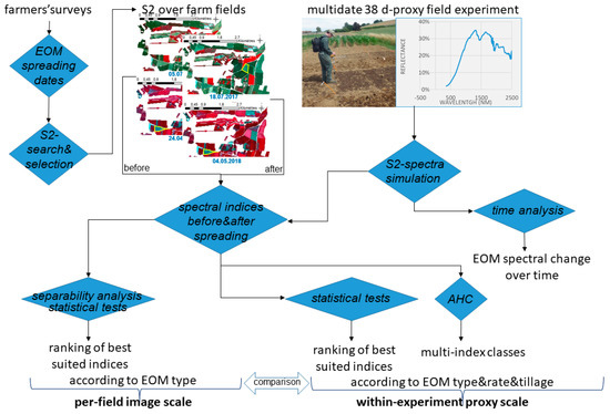
Figure 1.
Flowchart of the overall approach.
2.1. Satellite Image Reflectance Spectra
The Sentinel-2 series of the European Spatial Agency capture imagery in the visible, NIR and SWIR spectral ranges with a Multispectral Instrument (MSI) sensor. Sentinel-2 imagery with acquisition dates in close temporal proximity to the fertilization dates were downloaded from the Theia French land data center [33], which provides 10 spectral bands with 10 or 20 m spatial resolution: images are ortho-rectified, topographically and atmospherically corrected into surface reflectance through the MACCS-ATCOR Joint Algorithm (MAJA) processor [34] and delivered together with mask of cloud and their shadows (named “masque géophysique”, MG2 mask). The furthest acquisition dates considered were 5 days after EOM application (Table 1). In addition, rainfall on the day of image acquisition was considered (weather station of INRAE, Thiverval-Grignon) and rainfall amounts were null for all the images. In total, three images were selected and processed.

Table 1.
Sentinel-2 satellite imagery details.
The MG2 mask was applied to the imagery, a spatial subset of which was extracted using the French land parcel register of 2018 [35]. Then, based on previous observation in the Versailles plain [26], only bare fields were retained, i.e., having a Normalized Difference Vegetation Index value lower than 0.35.
2.2. Study Site Description
For testing Sentinel-2 images, six agricultural fields located in the Versailles plain, west of Paris (North of France, 48°46′–48°56′N; 1°50′–2°07′E) and covering about 10–20 ha each, were identified based on historical EOM amendment data. The most commonly cultivated crops in the area are wheat, corn and rapeseed. The fields pertain to three different soilscape units according to the 1/50,000 soil map of the region [26,36] characterized by the following soil types according to the FAO classification (World Reference Base (WRB), 2014 [37]): (1) on the flanks of an upper 180 m siliceous clay plateau (so-called “millstone”, with cavernous facies), podzolic arenosols and colluvic cambisols (three fields); (2) on a lower 120 m-limestone plateau wrapped with loessic deposits, haplic or truncated luvisols derived from loess (two fields including the control field); (3) on the flanks of this limestone plateau, rendzic, calcaric, or colluvic cambisols (two fields including the field experiment).
For characterizing the EOM spectral behavior through proximal reflectance measurements, a 60 m2—field experiment was performed in the AgroParisTech engineering school campus in Thiverval-Grignon, on an historical experimental field named “l’essai Dehérain” [38,39] (Figure 2). This field is characterized by a calcalric colluvic cambisol within a gentle and lower slope [39], pertaining to landscape unit 3. For the sake of the spectral measurements, sheep manure or green waste compost were applied in June–July 2020.
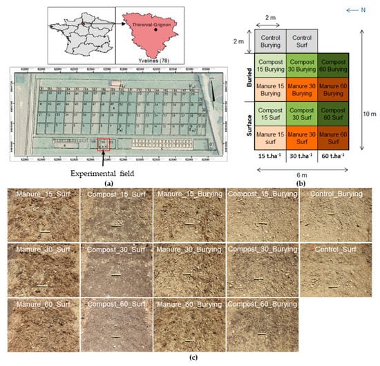
Figure 2.
Map of the experimental device Dehérain (Author Jean Marc Gilliot) in Thiverval-Grignon, with the field n°101 selected for this study (a), map of the experimental treatments (b) and Pictures showing the soil surface condition for all treatments (c). Control Burying/Surf, control field with/without tillage; Compost 15/30/60 Burying/Surf, green waste compost buried/without tillage at a rate of 15, 30, 60 t.ha−1, respectively; Manure 15/30/60 Burying/Surf, sheep manure buried/without tillage at a rate of 15, 30, 60 t.ha−1, respectively.
The farmers’ fields were amended with green waste compost or cattle manure, in addition to the control field which has not received EOM amendments for more than 30 years (Table 2). The application dates and rates were obtained by farmer surveys for July and August 2018. The average reflectance value of each field’s pixels was calculated for each spectral band and then compared between images before and after organic matter spreading.
Table 2.
Exogeneous organic amendment (EOM) data. Application date is approximated ±2 days.
2.3. Spectral Indices for EOM Detection
In total, five indices were computed, from both image spectra and field reflectance spectra simulated into Sentinel-2 spectral bands.
EOMI1 (Equation (1)) calculates the normalized difference of the B8A:B11 band ratio of Sentinel-2, which is analogous to the 5:4 band ratio of Landsat TM shown by Frazier and Cheng [40] to be strongly correlated (R2 = 0.98) to SOC. EOMI2 (Equation (2)) was adapted from the NDRI proposed by Gelder et al. [30]. EOMI3 (Equation (3)) combines EOMI1 and EOMI2 and enables to use the spectral bands of Sentinel-2 most impacted by EOM. EOMI4 (Equation (4)) is a normalized difference between the B11 and B4 bands. Finally, the fifth index (Equation (5)) was the Normalized Burn Ratio 2 (NBR2) which calculates the normalized difference of B11 and B12 bands and has previously been used to detect crop residue by Castaldi et al., 2019 [23].
For each field’s set of pixels, the histograms of indices values were compared before and after EOM application, then a separability index based on the Euclidean distances between these histograms was calculated. The index exhibiting the largest Euclidean distance before and after EOM application was chosen amongst these five for further investigation. In addition, a two-tailed Student’s t-test was applied to each index before and after with the null hypothesis of no significant difference between the distributions. The t-test was also applied for the control field.
2.4. Field Reflectance Experiment
To understand how EOM can impact soil reflectance, repeated spectral measurements of EOM applications were carried out within one bare soil field in the Dehérain experiment from 23 June to 30 July 2020 (Figure 2). We considered 14 treatments, covering a 2 m × 2 m square area each, according to three main criteria: (i) type of exogenous organic matter (Table 3), sheep manure or green waste compost; (ii) quantity of EOM application, according to three doses: 15, 30 and 60 tons of raw matter per hectare; (iii) cultural operation (tillage) after EOM application, consisting of burying or not burying the EOM with a rototiller. Two out of the 14 treatments were the control plots (no EOM spread), one with tillage and the other without tillage.
Table 3.
Main characteristics of green waste compost and sheep manure applied in the field experiment.
The EOMs were sampled for characterization at the time of application (Table 3). The sheep manure originated from a farm of Versailles plain (cattle manure was not available) while the green waste compost was produced from a composting plant. The quantities of EOM spread were chosen in accordance with the rate commonly applied in the Versailles plain: green waste compost and sheep manure are usually applied at a rate of 20–30 t.ha−1 [1]. Thus, 30 t.ha−1 represents our reference value. The rate of 15 t.ha−1 is seldom used, but in this study, it permits to observe a half dose. The rate of 60 t.ha−1 give the opposite information (double-dose). This rate is high but in Versailles plain, some farmers may spread green waste compost up to 100 t.ha−1. As many farmers bury EOM after spreading, the practice of tillage is intended to observe impact of burying. This is the reason why we realized our experimentation over the course of 38 days, through several (seven but only five were usable) successive reflectance measurements of all treatments. Rainfall was null and sky was perfectly clear on the three first days of experiment, then rainfall was close to null in the following days (Table 4). Due to erratic standard deviations, reflectance measurements of day 10 and 15 (cloudy) were not included in our analysis.
Table 4.
Rainfall data during the field experiment (INRAE weather station, Thiverval-Grignon).
Reflectance measurements were carried out with FieldSpec®3 (Analytical spectral Devises Inc., Boulder, CO, USA) and RS 3500® (Ltd. Spectral Evolution, Haverhill, MA, USA) portable spectroradiometers with 350–2500 nm spectral range for all treatments measurements after EOM spreading and for all treatments measurements before EOM spreading. The FieldSpec®3 spectral resolution is 3 nm in the 350–1000 nm region (sampling interval 1.4 nm) and 10 nm in the 1000–2500 nm region (sampling interval 2 nm). The RS 3500® spectral resolution is also 3 nm in the 350–1000 nm, 8 nm in the 1000–1900 nm and 6 nm in the 1900–2500 nm region. In order to minimize variations in illumination conditions and shadows effects related to soil roughness, the measurements were taken under conditions of few cumulus clouds between ± 2 h around solar noon. Both spectroradiometers have a 25° field of view, so that each reflectance at a 0.8 m-height integrates a spot size of about 0.1 m2 at nadir. Each field measurement was repeated by moving the spectroradiometer inside each treatment square. The values used at each site was an average of 60 or 70 spectra calibrated against a 30 cm × 30 cm and a 13 cm × 13 cm Spectralon® reflectance panel, for the Fieldspec® 3 and the RS 3500®, respectively. The RS 3500® was only used the first day of measurement before EOM spreading. Then, we used both pieces of equipment and retained the FieldSpec®3 spectra because the beam fixing the spectroradiometer’s pistol grip enabled a better distribution of spectral measurements for each treatment.
2.5. Analysis of Field Reflectance Spectra and of Temporal Indices Profiles
Field reflectance spectra of all treatments were acquired both before and after EOM spreading. For each measurement day, the spectra of all treatments were compared, in order to understand the spectral response according to the EOM and the quantity applied. The before-spectra aimed to characterize the spatial variations of bare soil across the field and verify its homogeneity. The after-spectra were taken the day of spreading and the 1st, 2nd and 3rd day and then until the 37th day after EOM spreading (Table 4). Because spectra of five treatments were inoperable for the 37th day, a total of 79 spectra were analyzed.
Field reflectance spectra were simulated into the MSI spectral bands of Sentinel-2, using a “read.asd” tool coded in Visual Basic for Application that enables to open field spectrum files in “.asd” format and to automate the pre-processing of spectra under the Excel® software. The “read.asd” tool averages spectra into 1 nm-intervals resulting in spectra with 2151 bands [41]. A recent update of the tool also permits to automatically weight average reflectance values using spectral sensitivities functions available for Sentinel-2 sensor. The five indices already used for image spectra were calculated from the simulated Sentinel-2 spectra.
To test the effect of EOM application, both ANOVA test and Tukey tests were applied between all treatments before and after EOM spreading.
Moreover, in order to discriminate between treatments, several multivariate approaches relied on calculating Ascending Hierarchical Clustering (AHC), with the Ward method [42], on either the simulated Sentinel-2 spectra, or on the spectral indices: (i) on the 14 observations of treatments before or after spreading for a given day, characterized by the 10 simulated spectral bands of Sentinel-2; (ii) for the same EOM spread rate over time, on the 20 observations and 10 variables; (iii) on all indices and 65 observations, which represented all treatments during the experimentation, for the purpose of observing their evolution over time.
3. Results
3.1. Analysis from Sentinel-2 Images the Days before and after
The application of green waste compost that occurred on four study fields around 28 July 2018 (Table 2) was traced by the acquisitions of 25 July and 2 August 2018 in perfect sky conditions. A strong reflectance decrease occurred in the visible and NIR regions after compost application (Figure 3). The largest decrease in image reflectance occurred in bands 8 and 8A, while the smallest appeared in band 12. The control field was unchanged in the visible bands, while displaying a slight reflectance decrease from B5 to B12 but within the range of values of non-amended soils.
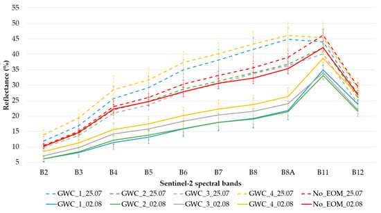
Figure 3.
Mean reflectance spectra of reference fields before (25 July) and after (2 August) green waste compost spreading of end of July 2018.
The application of cattle manure that occurred on two fields around 2 August 2018 (Table 2) was traced by the acquisitions of 2 and 4 August 2018 in perfect sky conditions. The spectral change observed between the two images suggests that fertilization did occur, either on 2 after satellite pass or on 3 August. The two Sentinel-2 images differ by a decrease in reflectance in the visible and NIR regions after EOM application (Figure 4). The reason for the different spectral profiles between the two amended fields might be due to the fact that one of the fields was tilled after fertilization (CM_1_Tilled). For the tilled field, the largest decrease in reflectance occurred in bands 8 and 8A, while the largest increase in reflectance occurred in band 12. The spectral difference of the non-tilled field (CM_2) shows the largest decrease in reflectance in bands 5, 6, 7, 8 and 8A and the largest increase in reflectance occurred in bands 11 and 12.
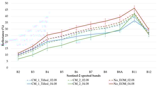
Figure 4.
Mean reflectance of sample fields before (2 August) and after (4 August) cattle manure amendment of beginning of August 2018. Both CM_1_Tilled and CM_2 received EOM, but the farmer also tilled and sowed a cover crop on the CM_1_Tilled.
The results of the Euclidean distance calculations between the before and after indices values distributions show that EOMI2 yields the largest statistical distance or separability for each EOM spreading event (Table 5). Even though the Euclidean distances between control fields were around 1.4, the EOMI1, EOMI3 and EOMI4 indices also yielded higher statistical distances than control, except EOMI4 for the CM_1_Tilled field. For both amendments, EOMI2 yielded the highest distance values before and after EOM spreading. Thus, the focus of the remaining analysis will be on EOMI2. EOMI2 values overall increased following both amendments, substantially for compost (Figure 5). Pixels for all three dates in the control field had a mean EOMI2 value of 0.10. Figure 4 displays the boxplots of EOMI2 before and after application. According to the two-tailed student’s t-test, the null hypothesis of no significant difference between distribution pairs shall be rejected, indicating statistically significant differences at α = 0.01. Null hypothesis was also rejected between the t-test of each “after EOM” and control (No_EOM) distribution, indicating statistically significant differences at α = 0.01. The CM_1_Tilled, which received cattle manure, showed the least difference between before and after EOM amendment, which might be due to tillage that was performed the same day of the EOM amendment.
Table 5.
Euclidean distances between before and after pixels distribution values of spectral indices for each studied field.
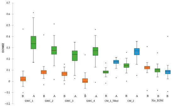
Figure 5.
Boxplots of EOMI2 pixels values before (B) and after (A) EOM amendment for each studied field. Sentinel-2 acquisition dates are 25 July 2018 (orange), 02 August 2018 (green) and 04 August 2018 (blue).
3.2. Analysis of Field Spectra before and after EOM Spreading over the First Three Days of Experiment
During the first day of the field experiment, before applying EOM, soil reflectance measurements acquired on bare soil suggest the spectral homogeneity of bare soil amongst the treatments (Figure 6). This spectral homogeneity was confirmed by the ANOVA test: indeed, all treatments were compared and no significant difference at α = 0.05 was shown by analysis of variance.
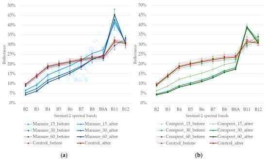
Figure 6.
Simulated Sentinel-2 reflectance spectra of the day 0 before amendment spreading (dotted line) and the day 2 after amendment spreading (full line) in surface according to EOM quantity (a) for green waste compost; (b) for sheep manure.
According to the results of the Tukey tests, simulated Sentinel-2 spectra show, for both green waste compost and sheep manure on the surface, a significant decrease of reflectance in the visible spectral bands (B2–B4) and a significant increase in the B11 SWIR band compared to bare soil (Figure 6b). Compared to bare soil, green waste compost spectra also show a significant decrease in the spectral bands B6, B7 and in the NIR spectral band B8, whereas reflectance of sheep manure either does not show a significant decrease or remains similar to bare soil for these bands. The difference between bare soil reflectance and EOM treatments is higher when the EOM quantity increases. However, reflectance spectra do not differ for EOM rates of 30 t.ha−1 and 60 t.ha−1 without tillage.
3.3. Analysis of Spectral Changes in the Field Experiment over the 38 Days Period
The multi-temporal observations show the change in reflectance over time for each treatment. Over the span of the spectral field experiment, the best index to monitor EOM was EOMI4. SWIR measurements analogous to spectral band B12 of Sentinel-2 were sometimes unusable because of disturbance and saturation, resulting in some inconsistent data for EOMI2 and EOMI3. Although EOMI4 was not the best performing index for monitoring EOM application in Sentinel-2 images, the results of the field experiment show this index to be sufficient to monitor EOM over time.
EOMI4 separates almost all applications of EOM from the control (Figure 7). According to the Tukey tests, only the buried green waste compost applied at a rate of 15 t.ha−1 does not show a statistical difference with the control treatments for D0 to D3. In addition, the index values reflect the quantity of EOM spread and the tillage. Specifically, the EOMI4 values are higher when the EOM is untilled and are positively correlated to the quantity of EOM applied.
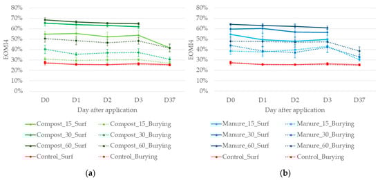
Figure 7.
Temporal change of EOMI4 values for all treatments. (a) Green waste compost; (b) sheep manure treatments. Dashed lines are for the Burying treatments.
3.4. Multi-Indices Grouping of the EOMs According to Type, Rate, Tillage
The AHC results obtained from the five indices (EOMI1, 2, 3, 4 and NBR2) for all spectral samples in the field experiment create four classes, successfully discerning between levels of EOM application (Figure 8). The first class regroups all control fields, all green waste compost burying at a rate of 15 t.ha−1 and sheep manure burying at a rate of 15 and 30 t.ha−1 for the day 37. The second and third classes contain the rest of the buried samples, mostly on the days shortly after EOM application and the sheep manure at a rate of 15 t.ha−1 in surface for the days 1 to 3. The last class collects all treatments with EOM in surface at a rate of 30 and 60 t.ha−1, as well as the manure in surface with a rate of 15 t.ha−1 for the day 0. The clustering of these samples into intuitive classes demonstrates the separative potential of these indices for detecting EOM amendments.
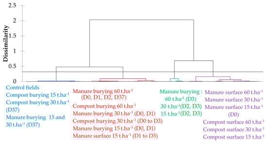
Figure 8.
AHC dendrogram of the indices for all treatments, over time (day after EOM application indicated in brackets, or not if all days are in the same class). Classes 1, 2, 3, 4 in blue, red, green, purple colors, respectively.
4. Discussion
This research pioneers the mapping of EOM amendment practices from optical remote sensing and especially from multispectral satellite images. The knowledge about such agricultural practices relies upon fastidious surveys of farmers; the bottleneck being the difficulty to retrieve the precise dates and hours of spreading, which are not always recorded. Previous research that is relevant and complementary to this topic dealt either with dry vegetation or crop residues (e.g., [31]), topsoil SOC (e.g., [22,23,25,43]), or tillage operations (e.g., [41]). Indeed, EOM amendments are left on soil surface in a similar way as dry vegetation or crop residues and they may be tilled just after spreading, thus, resembling tillage operations. However, conversely to dry vegetation or crop residues which can be left on surface over some weeks [31] and conversely to ploughing, that can be detected some months after [44], spreading events are time-limited, all the more when tillage is carried out for EOM burying. In addition, though the EOM incorporated into topsoil horizon contributes to increase topsoil SOC content, EOM detection may not be confused with SOC content detection: EOMs are spread as a thin additional layer on topsoils of different initial SOC contents, which are background material in the context of EOM detection.
4.1. A Promising Tool to Monitor EOM Amendment Practices
Exogenous organic matter amendments, such as green waste compost and cattle manure amendments, can be detected by Sentinel-2 images (Figure 9), particularly with the EOMI2 index. Other indices also yielded significant results, even though they were less performing than EOMI2. Our field spectral measurements confirmed significant results with simulated Sentinel-2 reflectance spectra. However, in this experiment the EOMI4 performed the best, perhaps due to noise component over the B12 spectral band which impacted the EOMI2 and EOMI3 index. Our field experimentation also exhibited that EOM amendments can still be detected until three days after spreading. Because the field measurements were carried out over areas too small to allow satellite observations, further study will consist of carrying out in situ measurements at the scale of agricultural plots.

Figure 9.
Infrared colored composite image (R:8, G:4, B:3) before (left) and after (right) green waste compost amendment. The fields with information on EOM spreading are delineated in yellow. White areas are non-agricultural areas.
Field measurements revealed that both green waste compost and sheep manure had distinct spectral response. Thus, a combination of several indices, rather one single index, could contribute to better identify the variety of EOM and even assess the quantity applied. However, as only two solid EOMs have been considered here, further research should include an evaluation of the performance of our indices for both other solid EOMs, such as other composts, manures and liquid EOMs, such as slurries or digestates.
In addition, the feasibility of an Earth observation monitoring from Sentinel-2 times series should be consolidated over larger periods encompassing crop rotations that is more than 4 years.
4.2. Remaining Issues for Tracking the Application of Exogenous Organic Matter
Organic amendments are applied only occasionally. Thus, the acquisition of Sentinel-2 images must be done shortly after organic matter application to avoid a shift in soil surface characteristics, which is not due to the EOM spreading. Indeed, vegetation growth, tillage operations and rainfall events occurring after EOM amendments may influence soil surface characteristics. The accurate identification of amendment application events depends on the availability of good quality images at key periods. Our field measurements showed that spectral indices were less effective 37 days after EOM application. Moreover, rainfall could explain the decrease of index values after three days, since it rained 1, 2.2 and 7 mm, respectively, on the 4th, 8th and 32th day after EOM spreading (Table 4) and this rainfall could have impacted soil moisture. Therefore, spectral changes occurring after three days still need further observations.
The field measurements were carried out in summer. Recent study has shown that the prediction performance of soil organic carbon was impacted by the acquisition date [25], notably due to soil roughness generated by ploughing, as well as soil moisture. Thus, the prediction performance of EOM amendments should also be tested in the spring and autumn in order to assess the influence of either soil roughness or soil moisture.
Lastly, we wish to emphasize that, except for the field experiment, the six fields under study through Sentinel-2 imagery were not experimental fields, but farmers’ fields, surveyed for their EOM spreading data information. For the purpose of mapping the spread fields, a more comprehensive survey of farmers would be needed, retrieving the precise dates and hours of spreading. According to the SOC map of the Versailles Plain realized by Zaouche and al., in 2017 [45], the “control” fields for no amendment spreading have a lower SOC content than organic amended fields, respectively less than 13 g.kg−1 and more than 17 g.kg−1. Thus, this study set out the capability of Sentinel-2 to follow two different EOMs and the spectral difference which can be detected with indices within the same field at the farm scale. However, further studies will have to be led with more field data in order to account for the possible background influence of soil type and topsoil SOC content.
5. Conclusions
This research is aimed to further facilitate the monitoring of amendment practices, which relies upon fastidious surveys of farmers; the bottleneck being the difficulty to retrieve the precise dates and hours of spreading, which are not always recorded. In this study, Sentinel-2 imagery showed strong potential for the detection of exogenous organic matter amendments at the farm scale. Image analysis before and after amendment application revealed the spectral changes in the visible, NIR and SWIR wavelengths. From this analysis, we identified five indices for analysis, of which EOMI2 created the most separation in each pair of images. Moreover, field reflectance measurements confirmed that green waste compost and sheep manure amendments could be detected at a minimum rate of 15 t.ha−1 on surface or buried for sheep manure and a minimum rate of 30 t.ha−1 for buried green waste compost. Field reflectance measurements also showed that green waste compost and sheep manure do not influence the same spectral bands of Sentinel-2. Over the timespan of the field experiment, the best index to monitor EOM was EOMI4. Thus, the use of one single simple index may not be adequate for the detection variation in EOM variety and quantity. Further study is necessary to improve the understanding of the spectral behavior of other EOM varieties in the field. Another further challenge will consist of gathering a more comprehensive survey of farmers in order to upscale such detection at a regional scale, while accounting for the possible background influence of soil type and topsoil SOC content.
Author Contributions
Conceptualization, M.D., E.V., F.L., H.D.S. and S.H.; methodology, M.D., H.D.S., E.V. and F.L.; validation, M.D., E.V. and F.L.; investigation, H.D.S. and F.L.; resources, H.D.S., D.H. and S.H.; Writing—Original draft preparation, M.D.; Writing—Review and editing, all co-authors; supervision, E.V. and F.L.; project administration, E.V.; funding acquisition, E.V. All authors have read and agreed to the published version of the manuscript.
Funding
This work was supported by CNES, France and was carried out in the framework of the POLYPHEME project through the TOSCA program of the CNES (grant number 200769/id5917). It also benefited an internship grant from the CLAND convergence institute in 2019, in addition to Maxence Dodin’s PhD grant from part of the French ministry for agriculture and food cares.
Informed Consent Statement
Not applicable.
Data Availability Statement
The data presented in this study are available on request from the corresponding author.
Acknowledgments
We wish to thank Jean-Marc Gilliot for making his recent update of the read.asd tool available, thus enabling us to simulate the MSI spectral bands. Special thanks to agricultural farmers of the Versailles Plain and the organic platform for their data and their providing of exogenous organic matters.
Conflicts of Interest
The authors declare no conflict of interest.
References
- Moinard, V.; Levavasseur, F.; Houot, S. Current and potential recycling of exogenous organic matter as fertilizers and amendments in a French peri-urban territory. Resour. Conserv. Recycl. 2021, 169, 105523. [Google Scholar] [CrossRef]
- Obriot, F.; Stauffer, M.; Goubard, Y.; Cheviron, N.; Peres, G.; Eden, M.; Revallier, A.; Vieublé-Gonod, L.; Houot, S. Multi-criteria indices to evaluate the effects of repeated organic amendment applications on soil and crop quality. Agric. Ecosyst. Environ. 2016, 232, 165–178. [Google Scholar] [CrossRef]
- Maillard, É.; Angers, D.A. Animal manure application and soil organic carbon stocks: A meta-analysis. Glob. Chang. Biol. 2014, 20, 666–679. [Google Scholar] [CrossRef]
- Rodrigo-Comino, J.; López-Vicente, M.; Kumar, V.; Rodríguez-Seijo, A.; Valkó, O.; Rojas, C.; Pourghasemi, H.R.; Salvati, L.; Bakr, N.; Vaudour, E.; et al. Soil Science Challenges in a New Era: A Transdisciplinary Overview of Relevant Topics. Air Soil Water Res. 2020, 13, 1178622120977491. [Google Scholar] [CrossRef]
- Chabbi, A.; Lehmann, J.; Ciais, P.; Loescher, H.W.; Cotrufo, M.F.; Don, A.; San-Clements, M.; Schipper, L.; Six, J.; Smith, P.; et al. Aligning agriculture and climate policy. Nat. Clim. Chang. 2017, 7, 307–309. [Google Scholar] [CrossRef]
- Soussana, J.-F.; Lutfalla, S.; Ehrhardt, F.; Rosenstock, T.; Lamanna, C.; Havlík, P.; Richards, M.; (Lini) Wollenberg, E.; Chotte, J.-L.; Torquebiau, E.; et al. Matching policy and science: Rationale for the ‘4 per 1000—Soils for food security and climate’ initiative. Soil Tillage Res. 2019, 188, 3–15. [Google Scholar] [CrossRef]
- Houot, S.; Pons, M.N.; Pradel, M.; Caillaud, M.A.; Savini, I.; Tibi, A. Valorisation Des Matières Fertilisantes d’origine Résiduaire Sur Les Sols à Usage Agricole Ou Forestier. Impacts Agronomiques, Environnementaux, Socio-Économiques. Expertise Scientifique Collective; INRA-CNRS-Irstea: Paris, France, 2014. [Google Scholar]
- ADEME Pays de la Loire. Matières Fertilisantes Organiques: Gestion et Épandage. In Clés Pour Agir; ADEME PAYS-DE-LA-LOIRE: Nantes, France, 2018; 14p, ISBN 979-10-297-0984-5. [Google Scholar]
- Tang, H.; Qiu, J.; van Ranst, E.; Li, C. Estimations of soil organic carbon storage in cropland of China based on DNDC model. Geoderma 2006, 134, 200–206. [Google Scholar] [CrossRef]
- Duretz, S.; Drouet, J.; Durand, P.; Hutchings, N.; Theobald, M.; Salmon-Monviola, J.; Dragosits, U.; Maury, O.; Sutton, M.; Cellier, P. NitroScape: A model to integrate nitrogen transfers and transformations in rural landscapes. Environ. Pollut. 2011, 159, 3162–3170. [Google Scholar] [CrossRef]
- Ben-Dor, E. The reflectance spectra of organic matter in the visible near-infrared and short wave infrared region (400–2500 nm) during a controlled decomposition process. Remote Sens. Environ. 1997, 61, 1–15. [Google Scholar] [CrossRef]
- Malley, D.F.; Yesmin, L.; Eilers, R.G. Rapid Analysis of Hog Manure and Manure-amended Soils Using Near-infrared Spectroscopy. Soil Sci. Soc. Am. J. 2002, 66, 1677–1686. [Google Scholar] [CrossRef]
- Malley, D.F.; Martin, P.D. The use of near-infrared spectroscopy for soil analysis. In Tools for Nutrient and Pollutant Management: Application to Agriculture and Environmental Quality, Occasional Report No. 17. Fertilizer and Lime ResearchCentre, Massey University, Palmerston North, New Zealand, December 2003; Currie, L.D., Hanly, J.A., Eds.; Winnipeg, MB, Canada, 2003; pp. 371–404. Available online: http://tur-www1.massey.ac.nz/~flrc/workshops/03dec/Abstract%20Malley.pdf (accessed on 1 January 2021).
- Réveillé, V.; Mansuy, L.; Jardé, E.; Garnier-Sillam, É. Characterisation of sewage sludge-derived organic matter: Lipids and humic acids. Org. Geochem. 2003, 34, 615–627. [Google Scholar] [CrossRef]
- Lashermes, G.; Nicolardot, B.; Parnaudeau, V.; Thuriès, L.; Chaussod, R.; Guillotin, M.L.; Lineres, M.; Mary, B.; Metzger, L.; Morvan, T.; et al. Indicator of potential residual carbon in soils after exogenous organic matter application. Eur. J. Soil Sci. 2009, 60, 297–310. [Google Scholar] [CrossRef]
- Jouraiphy, A.; Amir, S.; el Gharous, M.; Revel, J.C.; Hafidi, M. Chemical and spectroscopic analysis of organic matter trans-formation during composting of sewage sludge and green plant waste. Int. Biodeterior. Biodegrad. 2005, 56, 101–108. [Google Scholar] [CrossRef]
- Ben-Dor, E. Quantitative remote sensing of soil properties. In Advances in Agronomy; Elsevier BV: Amsterdam, The Netherlands, 2002; Volume 75, pp. 173–243. [Google Scholar]
- Vergnoux, A.; Guiliano, M.; le Dréau, Y.; Kister, J.; Dupuy, N.; Doumenq, P. Monitoring of the evolution of an industrial compost and prediction of some compost properties by NIR spectroscopy. Sci. Total Environ. 2009, 407, 2390–2403. [Google Scholar] [CrossRef] [PubMed]
- Ogen, Y.; Neumann, C.; Chabrillat, S.; Goldshleger, N.; Ben-Dor, E. Evaluating the detection limit of organic matter using point and imaging spectroscopy. Geoderma 2018, 321, 100–109. [Google Scholar] [CrossRef]
- Barthès, B.G.; Chotte, J. Infrared spectroscopy approaches support soil organic carbon estimations to evaluate land degradation. Land Degrad. Dev. 2021, 32, 310–322. [Google Scholar] [CrossRef]
- Gholizadeh, A.; Žižala, D.; Saberioon, M.; Borůvka, L. Soil organic carbon and texture retrieving and mapping using proximal, airborne and Sentinel-2 spectral imaging. Remote Sens. Environ. 2018, 218, 89–103. [Google Scholar] [CrossRef]
- Castaldi, F.; Hueni, A.; Chabrillat, S.; Ward, K.; Buttafuoco, G.; Bomans, B.; Vreys, K.; Brell, M.; van Wesemael, B. Evaluating the capability of the Sentinel 2 data for soil organic carbon prediction in croplands. ISPRS J. Photogramm. Remote Sens. 2019, 147, 267–282. [Google Scholar] [CrossRef]
- Castaldi, F.; Chabrillat, S.; Don, A.; van Wesemael, B. Soil Organic Carbon Mapping Using LUCAS Topsoil Database and Sentinel-2 Data: An Approach to Reduce Soil Moisture and Crop Residue Effects. Remote Sens. 2019, 11, 2121. [Google Scholar] [CrossRef]
- Vaudour, E.; Gomez, C.; Fouad, Y.; Lagacherie, P. Sentinel-2 image capacities to predict common topsoil properties of temperate and Mediterranean agroecosystems. Remote Sens. Environ. 2019, 223, 21–33. [Google Scholar] [CrossRef]
- Vaudour, E.; Gomez, C.; Loiseau, T.; Baghdadi, N.; Loubet, B.; Arrouays, D.; Ali, L.; Lagacherie, P. The Impact of Acquisition Date on the Prediction Performance of Topsoil Organic Carbon from Sentinel-2 for Croplands. Remote Sens. 2019, 11, 2143. [Google Scholar] [CrossRef]
- Vaudour, E.; Gomez, C.; Lagacherie, P.; Loiseau, T.; Baghdadi, N.; Urbina-Salazar, D.; Loubet, B.; Arrouays, D. Temporal mosaicking approaches of Sentinel-2 images for extending topsoil organic carbon content mapping in croplands. Int. J. Appl. Earth Obs. Geoinf. 2021, 96, 102277. [Google Scholar] [CrossRef]
- Žížala, D.; Minařík, R.; Zádorová, T. Soil Organic Carbon Mapping Using Multispectral Remote Sensing Data: Prediction Ability of Data with Different Spatial and Spectral Resolutions. Remote Sens. 2019, 11, 2947. [Google Scholar] [CrossRef]
- McNairn, H.; Protz, R. Mapping Corn Residue Cover on Agricultural Fields in Oxford County, Ontario, Using Thematic Mapper. Can. J. Remote Sens. 1993, 19, 152–159. [Google Scholar] [CrossRef]
- Qi, J.; Marsett, R.; Heilman, P.; Bieden-Bender, S.; Moran, S.; Goodrich, D.C.; Weltz, M. RANGES improves satellite-based information and land cover assessments in southwest United States. Eos 2002, 83, 601–606. [Google Scholar] [CrossRef]
- Gelder, B.K.; Kaleita, A.L.; Cruse, R.M. Estimating Mean Field Residue Cover on Midwestern Soils Using Satellite Imagery. Agron. J. 2009, 101, 635–643. [Google Scholar] [CrossRef]
- Van Deventer, A.P.; Ward, A.D.; Gowda, P.H.; Lyon, G.J. Using Thematic Mapper data to identify contrasting soil plains and tillage practices. Photogramm. Eng. Remote Sens. 1997, 63, 87–93. [Google Scholar]
- Demattê, J.A.M.; Fongaro, C.T.; Rizzo, R.; Safanelli, J.L. Geospatial Soil Sensing System (GEOS3): A powerful data mining procedure to retrieve soil spectral reflectance from satellite images. Remote Sens. Environ. 2018, 212, 161–175. [Google Scholar] [CrossRef]
- THEIA-LAND—Données et Services Pour les Surfaces Continentales. Available online: https://www.theia-land.fr/ (accessed on 16 April 2021).
- Baetens, L.; Desjardins, C.; Hagolle, O. Validation of Copernicus Sentinel-2 Cloud Masks Obtained from MAJA, Sen2Cor, and FMask Processors Using Reference Cloud Masks Generated with a Supervised Active Learning Procedure. Remote Sens. 2019, 11, 433. [Google Scholar] [CrossRef]
- Levavasseur, F.; Martin, P.; Bouty, C.; Barbottin, A.; Bretagnolle, V.; Thérond, O.; Scheurer, O.; Piskiewicz, N. RPG Explorer: A new tool to ease the analysis of agricultural landscape dynamics with the Land Parcel Identification System. Comput. Electron. Agric. 2016, 127, 541–552. [Google Scholar] [CrossRef]
- Crahet, M. Soil Map of the Versailles Plain. Scale 1:50 000; Internal Report; Institut National Agronomique Paris-Grignon, Grignon: Paris, France, 1992. [Google Scholar]
- World Reference Base (WRB). World Reference Base for Soil Resources. A Framework for International Classification, Correlation and Communication; Food and Agriculture Organization of the United Nations: Rome, Italy, 2014; p. 128. [Google Scholar]
- Houot, S.; Chaussod, R. Impact of agricultural practices on the size and activity of the microbial biomass in a long-term field experiment. Biol. Fertil. Soils 1995, 19, 309–316. [Google Scholar] [CrossRef]
- Baize, D.; Bourgeois, S. Estimation des apports agricoles et des retombées atmosphériques en éléments en traces et majeurs grâce à un essai de longue durée. Etude Gest. Sols 2005, 16, 9–23. [Google Scholar]
- Frazier, B.E.; Cheng, Y. Remote sensing of soils in the eastern Palouse region with Landsat Thematic Mapper. Remote Sens. Environ. 1989, 28, 317–325. [Google Scholar] [CrossRef]
- Vaudour, E.; Gilliot, J.; Bel, L.; Bréchet, L.; Hamiache, J.; Hadjar, D.; Lemonnier, Y. Uncertainty of soil reflectance retrieval from SPOT and Rapid Eye multispectral satellite images using a per-pixel bootstrapped empirical line atmospheric correction over an agricultural region. Int. J. Appl. Earth Obs. Geoinf. 2014, 26, 217–234. [Google Scholar] [CrossRef]
- Ward, J.H. Hierarchical Grouping to Optimize an Objective Function. J. Am. Stat. Assoc. 1963, 58, 236–244. [Google Scholar] [CrossRef]
- Vaudour, E.; Bel, L.; Gilliot, J.M.; Coquet, Y.; Hadjar, D.; Cambier, P.; Michelin, J.; Houot, S. Potential of SPOT Multispectral Satellite Images for Mapping Topsoil Organic Carbon Content over Peri-Urban Croplands. Soil Sci. Soc. Am. J. 2013, 77, 2122–2139. [Google Scholar] [CrossRef]
- Vaudour, E.; Baghdadi, N.; Gilliot, J.-M. Mapping tillage operations over a peri-urban region using combined SPOT4 and ASAR/ENVISAT images. Int. J. Appl. Earth Obs. Geoinf. 2014, 28, 43–59. [Google Scholar] [CrossRef]
- Zaouche, M.; Bel, L.; Vaudour, E. Geostatistical mapping of topsoil organic carbon and uncertainty assessment in Western Paris croplands (France). Geoderma Reg. 2017, 10, 126–137. [Google Scholar] [CrossRef]


Publisher’s Note: MDPI stays neutral with regard to jurisdictional claims in published maps and institutional affiliations. |
© 2021 by the authors. Licensee MDPI, Basel, Switzerland. This article is an open access article distributed under the terms and conditions of the Creative Commons Attribution (CC BY) license (https://creativecommons.org/licenses/by/4.0/).