How Can We Realize Sustainable Development Goals in Rocky Desertified Regions by Enhancing Crop Yield with Reduction of Environmental Risks?

Abstract

To meet the sustainable development goals in rocky desertified regions like Guizhou Province in China, we should maximize the crop yield with minimal environmental costs. In this study, we first calculated the yield gap for 6 main crop species in Guizhou Province and evaluated the quantitative relationships between crop yield and influencing variables utilizing ensembled artificial neural networks. We also tested the influence of adjusting the quantity of local fertilization and irrigation on crop production in Guizhou Province. Results showed that the total yield of the selected crops had, on average, reached over 72.5% of the theoretical maximum yield. Increasing irrigation tended to be more consistently effective at increasing crop yield than additional fertilization. Conversely, appropriate reduction of fertilization may even benefit crop yield in some regions, simultaneously resulting in significantly higher fertilization efficiency with lower residuals in the environment. The total positive impact of continuous intensification of irrigation and fertilization on most crop species was limited. Therefore, local stakeholders are advised to consider other agricultural management measures to improve crop yield in this region.

1. Introduction

In 2015, the UN Sustainable Development Goals (SDGs) provided a shared blueprint for peace and prosperity for people and the planet [1]. The second, sixth and fifteenth themes of this blueprint set specific goals for food security, clean water supply and halting land degradation [2]; requiring balancing of agricultural development and the environment [3]. Over the past decades, the intensification of irrigation and fertilization has greatly improved food production globally, but at the cost of environmental pollutions like soil salination and eutrophicated water resources [4,5]. The difficulty of achieving these SDGs is spatially unbalanced. This is especially evident for some underdeveloped areas due to their environmental and economical limitations [6]. For example, in karst regions, rocky desertification, a process of land degradation involving serious soil erosion, results in extensive exposure of basement rocks, a drastic decrease in soil productivity, and the appearance of a desert-like landscape [7,8,9]. The poor fertility of the edaphic environment, along withwater and soil losses, induces low crop productivity [10,11]. Nitrogen and other nutrition loss from the karst system also lead to lower nutrient use efficiency of vegetation and contaminates water quality, further impacting the long-term soil security and sustainability in karst regions [12].

Guizhou province, located in southwest China, contains large karst regions with their highly sensitive and vulnerable ecosystem and is one of the world’s largest exposed carbonate rock areas [13]. Guizhou has been a hotspot for research on karst geology, natural vegetation and agriculture for many years [14]. Due to the thinness, infertility of such soils and wide distribution of fragmented, sloping farmland in this region, the grain crop productivity per capita is only 337 kg for Guizhou Province, approximately 25% below the average value for the whole of China in 2016 [15]. In recent years, Guizhou has achieved rapid economic growth [16], partly through the intensification of agricultural practices involving the overuse of farmland and fertilization investment, exacerbating environmental degradation [17]. Meeting food demand is vitally important in Guizhou Province, where the birth rate has remained one of the highest in China. To achieve this goal, three approaches were widely applied previously in this area. First, the area of farmland was expanded by sacrificing the natural forest and other green lands [18,19]. However, this strategy was suspended in this region, under projects like the “Grain for Green” released in the 1990s to protect and restore natural vegetation [20], as local people and government began to realize the importance of natural vegetation in maintaining the local environment [21,22]. This program has generally been economically positive for most areas involved and also has addressed the environmental problems it set out to deal with, including reducing soil erosion and flooding [23]. Second, new crop species (e.g., hybrid rice) and planting/management patterns were imported into some areas of Guizhou Province to improve crop yield [24], but the spread and application were greatly constrained by the knowledge background and economic condition of each household in the local area. Third, improvement of crop yield is optimized by the investment of fertilization and irrigation, which is the most accessible intervention for each household. However, overuse of these two resources may lead to soil degradation, excessive fertilization and water wastage [25,26]. Therefore, appropriate irrigation and fertilization practices can reduce nutrient (e.g., N and P) loss, enhance crop growth and increase yields [27].

Despite changes in agricultural management strategies in Guizhou Province since the 1960s [28], the yield improvement of some staple crops like wheat and rice has stagnated by comparing yield data from 1985 and 2005 [29]. Therefore, agricultural management based on scientific evidence is key to realizing sustainable development, balancing environmental impact and food demand. Utilizing decision support tools (DST) can be integrated into political decision-making and the public realm, which will significantly benefit stakeholders in optimizing crop yield [30,31]. To evaluate the impact of different agricultural management strategies on crop yield, the concept of yield gap should be considered. The yield gap can be classified as either the difference in crop yield between the optimal experimental environment (without growth limitations) and the natural environment, or the yield potential in farmland over a specified spatial and temporal scale of interest [32]. Understanding the yield gap can help us to identify the potential scope for raising average yields via management changes [33,34].

Until now, the existing crop yield estimation models mainly contained statistical approaches and process-based models (including large-scale global gridded crop models) [35,36]. For statistical approaches, multiple linear regression [37,38] or piecewise linear regression [39] were widely utilized to build the mathematical relationship between crop yield and influencing factors to simulate the changes under different scenarios. Normally, statistical approaches use a few key inputs, such as meteorological variables, excluding other parameters (e.g., soil properties). However, the underground environment of the critical zone in karst region is complex, with multiple elements (such as limestone fissures) having a large impact on natural vegetation growth [40,41], as well as crop production, so this compromise may cause uncertainties in the models during practice [42]. In contrast, process-based models require different procedures for parameterization and calibration. However, the karst environment’s highly heterogeneous nature and the prevalence of small-scale subsistence farming in Guizhou impede the applicability of existing process-based models used for large-scale applications [43,44]. In recent years, the rise of deep learning methods, such as artificial neural networks (ANN), provides a new solution to identify the relationship of different factors and crop yield with nonlinear regressions [45]. Based on ANN training, higher accuracy in the simulation of crop yield could be achieved [46,47].

In this paper, we identified the current yield gap in Guizhou Province and investigate strategies to close this gap. We first calculated the yield gap for 6 dominant crop species grown in Guizhou Province. We subsequently employed ensembled back propagation (BP) networks to simulate the crop yield and fertilizer balance (defined as the difference of fertilization investment and demand for crop growth) in the study region by inputting different influencing variables inside the networks. Lastly, we forecast the variation in crop yield and fertilization efficiency under different agricultural management scenarios. The results of this work are useful as a DST for policymakers and other stakeholders to optimize food demand and environmental impact in agriculture development.

2. Data and Method

2.1. Study Region

Guizhou Province is located in southwest China, at the heart of the East Asia Karst, one of the three largest areas of almost unbroken karst globally [48] (Figure 1). There are 9 prefectures spatially distributed inside Guizhou. However, due to historical reasons and its geological environment, which causes difficulties with transportation and communication with outsiders, Guizhou is still one of the less developed provinces in China [49,50,51]. In this study, we chose 6 crops grown extensively in the 9 prefectures of Guizhou Province for the simulation of yield, which are maize, potato, rice, soybean and wheat (food crops), along with groundnut (cash crop).

2.2. Dataset

To simulate crop yield (per unit area), 14 variables were selected as input factors (

Table 1. Introduction of data resources (* crop-specific data).

Data	Dataset	Temporal Coverage	Spatial Resolution	References
Annual average temperature	WFDEI	1981–2016	0.5°	[53,54]
Annual average shortwave radiation
Annual total rainfall
Slope	GMTED2010 Global Grids	-	5′	[55,56]
Soil organic carbon	HWSD	1995	5′	[57,58,59]
Soil bulk density
Soil cation exchange capacity
pH
Carbonate content
Soil moisture	NCEP CPC	1948–present	0.5°	[60,61]
Irrigation	MIRCA2000 *	Circa 2000	5′	[62]
Crop area *	EarthStat	Circa 2000	5′	[63,64]
Crop yield *
N fertilizer rate *
P fertilizer rate *
K fertilizer rate *
N balance	EarthStat	Circa 2000	5′	[65]
P balance

, excluding crop yield, crop area, N and P balance), of which annual total rainfall, soil bulk density, irrigation, nitrogen (N) fertilizer rate, phosphorus (P) fertilizer rate and slope were chosen to simulate the Nor P balance. Specifically, we extracted all the data from (circa) year 2000 and unified their spatial resolution into 5′ by aggregation (overlaying meteorological data with a spatial resolution of 5° on 5′ data and extracted meteorological data values for each pixel of 5′). The dataset of crop yield was created by merging a detailed library of global census data (from the national, state and county level for over 20,000 political units) with three different, detailed satellite datasets of global landcover conditions, and this is by far the most complete dataset of agriculture [52].

2.3. Calculation of Yield Gap

To calculate the yield gap for the selected species, we referred to the approaches raised in the papers of Foley’s group [66]. First, we conducted an unsupervised spatial classification method (self-organizing feature mapping, or SOFM) to define different zones of “natural environment” (natural zones hereinafter) based on temperature, rainfall, shortwave radiation and slope, which human behaviors cannot change over a short period. This idea allowed us to control the same basic environmental conditions for crop growth. Inside each natural zone, we assumed that there is the same theoretical value of maximum crop yield, which is calculated based on the true yield distribution. Lastly, by comparing the true (observed) value with the theoretically maximum value, we finally calculated the yield gap in each prefecture.

2.3.1. SOFM

The SOFM network (Figure 2) consists of a fully interconnected array of neurons with a topology input layer and the competition layer [67]. The inputs are connected to each node on the network grid, and each grid node is only connected to adjacent nodes. They use a neighborhood function to preserve the input space’s topological properties and realize unsupervised classification by different data resources. The training process is completed to adjust the weight between each node in the output layer until it meets the fixed terminal condition. The whole process of this work is to reflect the input variables into lower dimensional space to realize the classification. The specific steps are as follows [68]:

(1)

Initializing each weight with a group of random numbers at the beginning;

(2)

Selecting the best matching unit. This step is also regarded as a competing process. The weight vector, which has the minimum Euclidean distance (calculated as below), with sample x (randomly selected), is the winning unit:

$$\Vert \mathrm{x}-{\mathrm{W}}_{\mathrm{c}}\Vert =\min \Vert {\mathrm{x}}_{\mathrm{i}}-{\mathrm{W}}_{\mathrm{i}}\Vert$$

(1)

where c represents the winning unit, and i is the sequence number for x and the weight vector;

(3)

Updating the weight until it meets the terminal conditions:

$$\mathrm{F}(\mathrm{i})=\exp (\frac{-{\Vert {\mathrm{p}}_{\mathrm{i}}-{\mathrm{p}}_{\mathrm{c}}\Vert }^2}{2{\mathsf{\sigma }}^2})$$

(2)

where p_i and p_c indicate the positions of the output units of i and c, respectively, while σ is the width of the neighborhood function.

2.3.2. Calculation of Yield Gap

The yield gap was calculated using three steps:

(1)

For each natural zone, the grid cells were sorted by their yield value, ranked from lowest to highest;

(2)

The grid cells’ respective harvested areas were accumulated into a histogram, then the percentile of 5th and 95th were extracted (Figure 3). The corresponding yield data from these two points were defined as theoretical minimum and maximum yield, indicating the potential yield for crops growing under purely natural conditions and under optimal agricultural management inside each zone. Extraction from the histogram of harvested area, instead of yield, can exclude the grid cells with too large or small cultivated areas that could skew the distribution of yield histogram;

(3)

For each grid cell, the crop yield gap was the difference between actual yield per area (AYPA) and potential yield per area (PYPA—referring to the theoretical yield under optimal growth conditions for each crop per area). Additionally, the yield gap of total production (AYPA/PYPA multiplied by corresponding cultivated area) was also calculated (shortened as AY and PA). To provide a better reference for policymakers and other stakeholders, we integrated each cell’s gap into the yield gap for each prefecture in Guizhou Province.

The theoretical maximum and minimum value also acted as the limiting threshold for further simulation of crop yield under different management scenarios.

2.4. Ensembled BP (Back Propagation) Artificial Neural Networks

2.4.1. Single BP Network

BP network is widely applied in classification, simulation and forecast across different research disciplines, and in our previous work it offered the best balance between accuracy in predicting crop yield in Guizhou Province and time cost [69,70]. This supervised learning is conducted using the mean square error and gradient descent algorithm to achieve the correction of the network connection weights, to minimize the difference between the mean square error of the actual output to achieve prediction accuracy. The common BP network structure consists of an input layer, (single or multiple) hidden layer (s) and an output layer. The BP process integrates the value of each node (or neuron) by weights, bias and activation function, then transfers this into the output layer, while the error signal is transmitted back along the original connection path, through the network, to modify the weights of neurons until the desired target is reached [71,72]. The training process can be characterized by numbers of iteration, and each run of them is called an epoch. Before commencing a BP network, several hyper-parameters, which may indirectly influence the accuracy and training efficiency of the model, need to be set, such as the numbers of hidden layers and nodes, as well as learning rate, etc. In this study, we imported one hidden layer with 10 nodes and used a tan-sigmoid (Equation (3)) function and linear function to transfer values between the different layers. Meanwhile, after testing different groups of hyper-parameters, the learning rate of the network and maximum epoch number was ultimately assigned as 0.01 and 5000, respectively.

$$\tan \mathrm{s}\mathrm{i}\mathrm{g}(\mathrm{x})=\frac{2}{\left(1+\exp (-2\mathrm{x})\right)}-1$$

(3)

2.4.2. Evaluating Accuracy of Simulation

The dataset was first randomly grouped into training data (75% of all data) and validation data (the remaining 25%). Three indices of validation data were selected to evaluate the accuracy of training performance of the BP network, including the correlation coefficient (between the true (observed) value and forecasted (simulated) value of the validation group), root-mean-square error (RMSE) and relative mean error (RME), the latter two, of which indicate absolute and relative deviation of the simulation results, respectively (defined in Equations (4) and (5)).

$$\mathrm{RMSE}=\sqrt{\frac{{\displaystyle {\sum }_{\mathrm{i}=1}^{\mathrm{n}}{({\mathrm{T}}_{\mathrm{i}}-{\mathrm{F}}_{\mathrm{i}})}^2}}{\mathrm{n}}}$$

(4)

$$\mathrm{RME}=\frac{{\displaystyle {\sum }_{\mathrm{i}=1}^{\mathrm{n}}\left|{\mathrm{T}}_{\mathrm{i}}-{\mathrm{F}}_{\mathrm{i}}\right|}}{\mathrm{n}}\times 100\%$$

(5)

where T and F represent true value and forecasted value, and n indicates the total number of validation samples.

2.4.3. Ensemble Approach

The ensemble approach for ANN is to integrate a finite number of ANNs that are trained for the same purpose whose predictions are combined to generate a unique output (Figure 4). The relationship between a group of ensembled ANNs and a single ANN is similar to a random forest and each tree inside. These ensembles have several advantages over a single ANN as they have the potential for improved generalization and increased stability, although at the cost of a longer training time, enabling better convergence and accuracy [73]. The commonly used idea of an ensemble approach to gain a final result from a group of ANNs can be categorized into “bagging” and “boosting”. They both build a robust classification or regression network based on a single ANN but with different specific algorithms [74]. Herein, for each process of simulation, we utilized the idea of “bagging”. Namely, we created several networks (the number of which was set following performance testing of the simulation—detailed in Section 2.4.4) and subsequently calculated the average value for each as the final result of the simulation, and this is the commonly used nonlinear regression model ensemble algorithm.

2.4.4. Scenario Settings and Convergence Test of Ensembled ANNs

To evaluate different future scenarios of agricultural management, we changed the input of N&P fertilizer (by ±10%) and irrigation rates (only by +10%, as the study region was proven to be lacking water resources for crops in previous studies) to explore the variation in crop yield in the 9 different prefectures of Guizhou Province. Moreover, we calculated the fertilization efficiency (FE) defined in Equation (6) to evaluate the comprehensive impact on both crop growth and the environment.

$$\mathrm{FE}=\frac{{\displaystyle \sum _{\mathrm{i}=1}^6{\mathrm{Y}}_{\mathrm{i}}\times {\mathrm{A}}_{\mathrm{i}}}}{\mathrm{N}(\mathrm{P}) \mathrm{balance}}$$

(6)

Here, Y is the yield per area for each selected crop species (6 in total), A represents the corresponding cultivated area. In a specific region, FE was calculated as total crop production divided by total N or P balance. A higher FE indicates the strategy of fertilization is more effective and reasonable, with the significant promotion of crop growth and low environmental cost.

The convergence test determines the final number (n) of BP networks brought into the ensemble method. The indicator for testing the convergence was set as the percentage of pixels with a 5–10% increase of yield after increasing N&P fertilizer and irrigation rates. The specific process of this method can be divided into four steps:

(1)

The number (n) of BP ANN was set from 1 to 40, respectively;

(2)

For each number of n, we built ensembled ANNs and ran the simulation 10 times;

(3)

After 10 simulations, we evaluated the performance of the ensemble by calculating the value of the defined indicator, correlation coefficient and time cost;

(4)

We compared the performance of ensembled ANNs to determine the final n for further simulations.

The optimization of n in the ensembled group can help us balance simulation stability with the time cost.

3. Results

3.1. Simulation of Single BP Network

To build the ensemble model, we first examined the simulation of crop yield per area and N, P balance by a single BP network with the yield influencing parameters detailed in Methods. The simulation for N, P balance is better than that for crop yield, with correlation coefficients (between the true value and fitted value) larger than 0.99 (Figure A1 in Appendix A). In contrast, the crop yield simulation accuracy varied among different species. For example, groundnut simulation had the best performance, indicated by the largest R (0.87) and least RME (11.67%), compared with the worst performance for potato (with R of 0.68 and RME of 15.38%). In terms of the time cost, the process of simulation of N or P balance is less than that of crop yield, about 2–3 (s) for training each network, while the time cost for simulation of crop yield ranges from 11.1 (s) to 19.7 (s) (Figure A1).

3.2. Convergence Test for Ensembled Networks

As introduced in Section 2.4.4, we used the change of crop yield (with an interval of increase of 5–10%) after changing the investment of N&P fertilizer and irrigation as an indicator to test the stability and convergence of ensembled BP networks. The number of networks in each ensembled group ranged from 1 to 40, and each group was conducted 10 times to analyze the distribution of the simulation results (detailed in Methods). Considering the efficiency of the process, we set the epoch number to 5000 for each time. In Figure A2 and Figure A3 we can see that when the number of networks is less than 10, the simulation results fluctuated greatly in terms of the indicator percentage. For example, when there is only one network in the ensemble (under the scenario of increasing N&P fertilizer), the indicator would range from 0.047 to 0.133, and with the increase of networks in the group (mostly > 30), the indicator reached a relatively stable value. The correlation coefficient (R; of the true and fitted value) followed a similar trend as the indicator. However, the convergence of R was achieved earlier than the indicator when networks exceeded 20. Lastly, the time cost of training the ensembled networks rose linearly or exponentially with the increasing number of networks. Balancing the time cost with the robustness of the simulation, we ultimately chose the group with 40 independent single BP networks and averaged the results for each as the final result of simulation and prediction of crop yield under different scenarios.

3.3. Yield Gap in Guizhou Province

The extent of yield gap (or potential yield) varied among the different pairs of crop and prefecture, with some crop species having relatively more potential for yield improvement in some of the prefectures compared with others. For example, the total yield gap of potato in Bijie and Guiyang is 365,666.0 (t) and 17,665.9 (t), respectively (Figure 5). Meanwhile, the ratio of actual yield and theoretical yield represents the proportion of local crop production that has achieved its maximum value. It can be seen that rice had the greatest ratio among the different crops, achieving more than 60% of the theoretical maximum yield per area and 72% for total yield in all the prefectures. By contrast, the yield per area of groundnut in Liupanshui and Qiandongnan only reached 47% and 52% of the theoretical maximum value. Lastly, the spatial difference of the ratio of maize is large, shown by the value of 88% in Bijie, but only 53% in Qiandongnan for the total production. This average percentage of achieved total production is all over 60% for each crop species in Guizhou, with a total mean value of 72.5% for all the selected crops.

3.4. Crop Yield and Fertilization Efficiency under Different Scenarios

After training the ensembled networks, we first increased the input variables of N&P and irrigation by 10% and predicted the variation of crop yield and fertilizer balance. On the whole, the change in yield was both crop- and prefecture-specific. Increasing fertilizer application benefited the yield (per area) of potato in most prefectures, except for Anshun, where potato yield decreased (Figure 6a). In particular, potato yield in Zunyi increased the greatest by 2.59 (t/ha). By contrast, other crops like maize in Zunyi, Bijie and Tongren decreased under the same scenario, although the degree of change was less than that of the increase in potato yield. The intensification of fertilization also caused the increase of N, P balance in all prefectures, with an average total increase in N of 8045.8 (kg/grid) and P of 1614.6 (kg/grid) in Guizhou. The increase in N and P balance was highly correlated in all prefectures (Figure A7). Moreover, even though some crop yields increased in this scenario, the total FE in all prefectures decreased, except for Bijie (Figure 6c). On the other hand, implementing an increase in irrigation by 10% could favor the growth of crops in most cases (Figure 6b). The average rise of yield per area is 0.54 (t/ha) and 0.47 (t/ha) for potato and rice. Spatially, however, the impacts are highly heterogeneous, as shown by the significant yield increase in Qianxinan, Qiandongnan and Qiangnan, with an average increase of 0.064 (t/ha), 0.031 (t/ha) and 0.027 (t/ha) for all crops, whereas the yield increase in Guiyang, Anshun and Tongren is negligible (detailed distribution of yield change in each prefecture illustrated in Figure A4 and Figure A5).

In the scenario of decreasing N&P fertilizer, the change in crop yield varied both spatially and for the species distribution (Figure 7a). Similarly to the former scenario, potato yield was the most impacted by changing the quantity of fertilization. Except for Qianxinan and Qiannan, the absolute yield decrease ranged from 1.94 t/ha (Tongren) to 0.28 t/ha (Zunyi) across Guizhou Province. By contrast, maize yield even showed a small increase following decreasing fertilizer investment, which is significant in mid-eastern prefectures like Zunyi, Tongren and Qiandongnan. Spatially, the greatest reduction in crop yield following fertilization reduction was shown in some southwestern prefectures (e.g., Anshun and Liupanshui). The decrease of all crop yields in Anshun ranged from 0.10 t/ha (groundnut) to 0.34 t/ha (potato). Moreover, the N, P balance also showed a synchronous shift after decreasing fertilization. The decline of N balance ranged from 13,605.0 kg/grid (Guiyang) to 4736.7 kg/grid (Qiandongnan), while P balance decreased much less (from 2894.3 kg/grid in Guiyang to 948.8 kg/grid in Qiandongnan). This phenomenon was following the former scenario. Moreover, it is worth noting that there is an evident spatial coherency for the change in N, P balance in Guizhou Province (R > 0.99), which implied that these shifts were mainly determined by the local environmental conditions, under the same change of fertilization. Lastly, this strategy demonstrated strong optimization on FE, shown by an increased value for all prefectures, except for Liupanshui, which had no significant variation in this scenario (Figure 7b; detailed distribution of yield change in each prefecture was illustrated in Figure A6).

3.5. Yield Gap Closing

Finally we calculated the ratio of (total) crop yield variation and (total) yield gap obtained from the ensemble networks and investigated the influence of intensifying management strategies (N&P fertilizer and irrigation combined) on closing the existing local yield gap. The impacts on the yield gap were both species and spatially heterogeneous (Figure 8). From a species perspective, potato and soybean gained the most crop yield, reducing the yield gap by an average of 33.9% and 16.6%, respectively. However, the yields of groundnut and maize decreased following additional agricultural investment, with an average reduction of −7.6% and −7.4%. From a spatial perspective, most crops in southern parts of Guizhou Province in Qiangdongnan, Qianxinan and Qiannan benefited from closing the yield gap by increasing N&P fertilizer and irrigation, where the averaged ratio value is 17.2%, 15.0% and 4.0%, respectively. At the same time, other prefectures had more heterogeneity in their yield gap variation.

4. Discussion

Establishing the quantitative relationship between crop yield and the environment is essential for understanding each factor’s interaction and predicting future crop yield under different climate or agricultural scenarios. Previously, these demands were mainly met by conducting different regression models or process-based models [37,38,75]. Nevertheless, these approaches have three issues. First, the performance of traditional models relied on the characteristics of the data distribution. For example, higher accuracy can be obtained when the crop yield variation is large [76]. Second, the large differences occurred between existing model outputs for simulating crop yield, and the relative error in some cases surpassed 50% [35]. Third, the reported accuracy for traditional regression and process-based models could only explain 51% and 42% of observed yield variability, respectively [77]. The technology of machine learning, including ANN, can counter these deficiencies to some extent. However, in previous studies, researchers have been cautious about predictions of crop yield under different scenarios by trained networks [31,37,45]. Most of these studies were constrained to fitting the existing crop yield; thus the work of prediction was mainly finished by existing traditional models [78,79,80]. Utilizing the characteristics of convergence of ensemble networks, we found that the usage of a single network may generate issues in terms of the stability of the result, revealed by the fluctuation of correlation coefficient of actual yield and fitted value. Namely, the correlation coefficient for each simulation can be high, but the distribution of the fitted value may vary dramatically, which was demonstrated by the indicator value fluctuating (Figure A2 and Figure A3). This issue could be prominent, especially when we conducted the prediction by a single network. Clustering of multiple networks (forming ensembled networks) can resolve these issues, providing a more reliable forecast of crop yield under future scenarios, but the time cost should also be fully considered.

To date, two main approaches are commonly used for estimating crop yield gaps in specific locations. The first is to apply crop models to set optimal environmental parameters to calculate the potential yield and gain the difference between the result with actual yield [81,82]. This method requires comprehensive environmental parameters throughout the growing season for each crop (often with daily temporal resolution), relying on the availability of historical data records. In contrast, the second method, which we employed in this study, calculates the yield gap by statistical data. This method is simple to conduct and fully considers the actual yield to obtain the locally exploitable yield gap. However, previous studies utilizing this method only imported variables of temperature elements to classify natural zones [52]. To strengthen our analysis, we added shortwave radiation, rainfall and slope as well in this study. Particularly, slope (representing topography and, therefore, areas of severe soil degradation in the region) has been proven to be the main factor for limiting the absorption of water and nutrient resources belowground for vegetation (including crop) growth in the karst region [9,83]. Therefore, this approach enables our subsequent analyses and conclusions for agricultural management to be more reliable.

In the past, large-scale yield gap studies have demonstrated a big difference between the yield gap in developed and developing countries, which means that some countries like European countries have achieved a high percentage of maximum yield in the local environment, while others have more scope to further increase local crop production [34]. This phenomenon was mainly caused by the imbalance of economic development and the spread of new agricultural techniques among different countries. For example, in Nebraska, USA, the production of maize has reached nearly 90% of the theoretical maximum, while in some African countries, this value is even less than 50% [84,85]. By contrast, the yield (per area) gap of maize in Guizhou was roughly ranked in between these two groups, ranging from 46% in Qiandongnan to 89% in Bijie. Meanwhile, the growth in crop yield in some areas has slowed in recent years, like maize in African countries and rice in the southern part of China [29]. Therefore, closing the yield gap by different approaches in these regions requires further investigation, especially in less developed areas [85].

For most crop species (excepting potato) in Guizhou Province, we found that the effect of fertilization has reached a tipping point, whereby increasing inputs of fertilizer alone will not achieve a significant rise in yield. Indeed, for some crops, additional fertilizer investment could even cause a reduction in crop yield (Figure 6a). Three reasons can explain this. First, the absorption of nutrient elements for crops like wheat has reached “saturation” in the soil, resulting in a low additional increase of absorption being detected after the fertilization tipping point is reached [86]. Second, the facilitation of crop growth via fertilization requires reasonable consideration of the ratios of different fertilizers (N, P and K) specific to the local area’s nutrient limitations and the crop species physiology, rather than a prescribed addition of each [87]. Third, the overuse of inorganic fertilizers can lead to negative environmental consequences, indicated by hardening of the soil, decreasing fertility, strengthening pesticides, polluting air and water resources, which further influences crop growth and production [88]. Therefore, more fertilization on crops in Guizhou Province could only cause more fertilizer balance left in the environment and less fertilization efficiency, further resulting in more environmental problems, which is illustrated by Figure 6c. According to statistics, average chemical fertilizer (N, P, and K) and pesticide use per hectare of cropland in China are between double and three times that of other countries/regions in the world [89]. Field surplus nitrogen (N) and farm disposal N are major sources of water pollution in farming systems, which contaminates the water supply for livelihood [90]. Hence, it is very important to manage the investment of different agricultural chemicals more precisely and more rationally. Our results also demonstrated that an appropriate reduction in fertilizer use might benefit the crop yield in some regions, as well as causing an evident increase in fertilization efficiency. For example, higher maize production in some mid-eastern prefectures existed with a distinct decrease in the N, P balance in Guizhou Province. However, the implementation of this strategy should fully consider the spatial heterogeneity. Among all the prefectures, Qianxinan was highly recommended to reduce fertilization, resulting in slightly higher crop yield, reduced fertilizer balance and agricultural management cost savings.

Furthermore, an appropriate increase of irrigation is able to favor crop yield in Guizhou Province, aside from the economic and natural resources costs involved (Figure 6b). The lack of water resources for crops in Guizhou karst farmland was also shown by the high crop water stress index for irrigation due to seasonal rainfall shortage and aggravated by the thin soil layer and poor water holding capacity in this area [91]. Although the impact of changing irrigation was less significant than that of fertilization (e.g., the increase of yield for potato by increasing irrigation is less than that from increasing fertilization), it has a more stable and positive consequence for most species in most regions. Compared with irrigation rates in the North China Plain and other northern farming areas, rainfed farmland accounted for a high percentage in southwest China. This region may also encounter additional water scarcity under global warming [92]. Therefore, considering the local topography, fragmentation of cropland, and other environmental characteristics, the combination of both “soft-path” (capturing water resources in small and check dams) and “hard-path” (with large, centralized, capital intensive irrigation projects and water storage infrastructure) may be necessary to enable sufficient irrigation water to meet the demand for crop growth in the future [93]. Moreover, it is notable that the implementation of these development patterns is often limited by “economic water scarcity” resulting from the cost of building irrigation infrastructure under local financial conditions [94].

Together, the continuous increase of fertilization and irrigation have a relatively limited effect on improving crop yield in Guizhou Province, except for potato and soybean. These indications can be used as a DST to target agricultural management to the areas where it will be most effective, and the stakeholders should consider other strategies to meet the local food demand. For example, optimizing plant developmental features, cross-breeding and hybridization, new genetic techniques and ecological engineering strategies, such as increasing biodiversity and soil fertility in farmland to harmonize agricultural development and the environment [95,96,97].

Other than the scale effect and errors brought by different spatiotemporal remote sensing datasets, this study’s uncertainty was also caused by the “extrapolation” effect of ANNs. Indeed, just like traditional regression models, the simulation accuracy of a neural network also relies on the distribution of training and input data for simulation. Where there is limited training data (e.g., the input data for prediction is beyond the range of training), the corresponding trained network tends to have an arbitrary prediction or classification [98], which can reduce the accuracy of the predictions. Different from the traditional classification of computer graphics or remotely sensed images [99,100], we often set future scenarios for environmental parameters (like increasing fertilization and irrigation in this study or higher global temperature) beyond that found in historical records, which may put the data out of the range of the available training data in the region and further impact the accuracy of the predictions. This error may also be expanded if there are large differences between the data utilized for prediction and the available training data [101]. Therefore, we only set the absolute rate of change at 10% for fertilization and irrigation.

5. Conclusions

In this paper, we calculated the yield gap for 6 crop species grown in Guizhou Province and used ensembled ANNs to predict the change in crop yield in Guizhou under different management scenarios of increasing/decreasing fertilization and irrigation. The conclusions are as follows:

(1)

The ensemble of ANNs can improve the robustness of simulation of crop yield by multiple input factors, which is especially beneficial for predictions under different future scenarios;

(2)

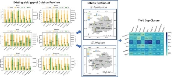
The selected crops’ total yield has already realized over 60% for each of the theoretical maximum, with an average value of 72.5% in all cases. The yield gap in the study area is still larger than that in most developed countries;

(3)

An appropriate increase in irrigation can benefit the crop yield for most Guizhou species, compared with increasing fertilization. Moderate reduction of fertilizer in this region may increase some crop production and enhance local fertilization efficiency. Combing the management strategies of increasing fertilization and irrigation was beneficial for increasing the yield of potato and soybean, but this approach has a limited effect on the existing yield gap for most other crops in Guizhou Province.

References

1. World Health Organization. Health in 2015: From MDGs, Millennium Development Goals to SDGs, Sustainable Development Goals; World Health Organization: Geneva, Switzerland, 2015. [Google Scholar]
2. Dhahri, S.; Omri, A. Foreign capital towards SDGs 1 & 2—Ending Poverty and hunger: The role of agricultural production. Struct. Change Econ. Dyn. 2020, 53, 208–221. [Google Scholar]
3. McNeill, D. The contested discourse of sustainable agriculture. Glob. Policy 2019, 10, 16–27. [Google Scholar] [CrossRef] [Green Version]
4. Li, J.; Pu, L.; Han, M.; Zhu, M.; Zhang, R.; Xiang, Y. Soil salinization research in China: Advances and prospects. J. Geogr. Sci. 2014, 24, 943–960. [Google Scholar] [CrossRef]
5. Huang, J.; Xu, C.-C.; Ridoutt, B.G.; Wang, X.-C.; Ren, P.-A. Nitrogen and phosphorus losses and eutrophication potential associated with fertilizer application to cropland in China. J. Clean. Prod. 2017, 159, 171–179. [Google Scholar] [CrossRef]
6. Wang, Y.; Lu, Y.; He, G.; Wang, C.; Yuan, J.; Cao, X. Spatial variability of sustainable development goals in China: A provincial level evaluation. Environ. Dev. 2020, 35, 100483. [Google Scholar] [CrossRef]
7. Wang, S.J.; Liu, Q.M.; Zhang, D.F. Karst rocky desertification in southwestern China: Geomorphology, landuse, impact and rehabilitation. Land Degrad. Dev. 2004, 15, 115–121. [Google Scholar] [CrossRef]
8. Zhang, Z.-H.; Hu, G.; Ni, J. Effects of topographical and edaphic factors on the distribution of plant communities in two subtropical karst forests, southwestern China. J. Mt. Sci. 2013, 10, 95–104. [Google Scholar] [CrossRef]
9. Zhang, Z.H.; Hu, G.; Zhu, J.D.; Luo, D.H.; Ni, J. Spatial patterns and interspecific associations of dominant tree species in two old-growth karst forests, SW China. Ecol. Res. 2010, 25, 1151–1160. [Google Scholar] [CrossRef]
10. Zhang, W.; Chen, H.-S.; Wang, K.-L.; Su, Y.-R.; Zhang, J.-G.; Yi, A.-J. The heterogeneity and its influencing factors of soil nutrients in peak-cluster depression areas of karst region. Agric. Sci. China 2007, 6, 322–329. [Google Scholar] [CrossRef]
11. He, C.; Xiong, K.; Li, X.; Cheng, X. Karst geomorphology and its agricultural implications in Guizhou, China. In Proceedings of the Fourth International Conference on Geomorphology, Bologna, Italy, 28 August–3 September 1997. [Google Scholar]
12. Song, X.; Gao, Y.; Green, S.M.; Dungait, J.A.J.; Peng, T.; Quine, T.A.; Xiong, B.; Wen, X.; He, N. Nitrogen loss from karst area in China in recent 50 years: An in-situ simulated rainfall experiment’s assessment. Ecol. Evol. 2017, 7, 10131–10142. [Google Scholar] [CrossRef] [PubMed]
13. Tong, X.; Brandt, M.; Yue, Y.; Horion, S.; Wang, K.; De Keersmaecker, W.; Tian, F.; Schurgers, G.; Xiao, X.; Luo, Y. Increased vegetation growth and carbon stock in China karst via ecological engineering. Nat. Sustain. 2018, 1, 44–50. [Google Scholar] [CrossRef]
14. Bai, G.-X.; Zhao, Z.; Qiu, H.-B. Studies on the germplasm resource diversity of drought-resistant maize in Guizhou. Agric. Res. Arid Areas 2007, 25, 1–4. [Google Scholar]
15. NBSC (National Bureau of Statistics of China). Statistical Yearbook of China; Chinese Statistics Press: Beijing, China, 2016. (In Chinese)
16. Zheng, Y.; Naylor, L.A.; Waldron, S.; Oliver, D.M. Knowledge management across the environment-policy interface in China: What knowledge is exchanged, why, and how is this undertaken? Environ. Sci. Policy 2019, 92, 66–75. [Google Scholar] [CrossRef]
17. Green, S.M.; Dungait, J.A.; Tu, C.; Buss, H.L.; Sanderson, N.; Hawkes, S.J.; Xing, K.; Yue, F.; Hussey, V.L.; Peng, J. Soil functions and ecosystem services research in the Chinese karst Critical Zone. Chem. Geol. 2019, 527, 119107. [Google Scholar] [CrossRef] [Green Version]
18. Gutiérrez Rodríguez, L.; Hogarth, N.J.; Zhou, W.; Xie, C.; Zhang, K.; Putzel, L. China’s conversion of cropland to forest program: A systematic review of the environmental and socioeconomic effects. Environ. Evid. 2016, 5, 1–22. [Google Scholar] [CrossRef] [Green Version]
19. Zabel, F.; Delzeit, R.; Schneider, J.M.; Seppelt, R.; Václavík, T. Global impacts of future cropland expansion and intensification on agricultural markets and biodiversity. Nat. Commun. 2019, 10, 2844. [Google Scholar] [CrossRef] [Green Version]
20. Song, X.; Peng, C.; Zhou, G.; Jiang, H.; Wang, W. Chinese Grain for Green Program led to highly increased soil organic carbon levels: A meta-analysis. Sci. Rep. 2014, 4, 4460. [Google Scholar] [CrossRef] [Green Version]
21. Feng, Z.; Yang, Y.; Zhang, Y.; Zhang, P.; Li, Y. Grain-for-green policy and its impacts on grain supply in West China. Land Use Policy 2005, 22, 301–312. [Google Scholar] [CrossRef]
22. Yang, J.; Xu, X.; Liu, M.; Xu, C.; Zhang, Y.; Luo, W.; Zhang, R.; Li, X.; Kiely, G.; Wang, K. Effects of “Grain for Green” program on soil hydrologic functions in karst landscapes, southwestern China. Agric. Ecosyst. Environ. 2017, 247, 120–129. [Google Scholar] [CrossRef]
23. Delang, C.O.; Yuan, Z. China’s Grain for Green Program; Springer: Cham, Switzerland, 2016. [Google Scholar]
24. Zhang, D.; Min, Q.; Liu, M.; Cheng, S. Ecosystem service tradeoff between traditional and modern agriculture: A case study in Congjiang County, Guizhou Province, China. Front. Environ. Sci. Eng. 2012, 6, 743–752. [Google Scholar] [CrossRef]
25. Khan, S.; Anwar, S.; Kuai, J.; Ullah, S.; Fahad, S.; Zhou, G. Optimization of Nitrogen Rate and Planting Density for Improving Yield, Nitrogen Use Efficiency, and Lodging Resistance in Oilseed Rape. Front. Plant Sci. 2017, 8, 532. [Google Scholar] [CrossRef] [PubMed] [Green Version]
26. Mahajan, G.; Chauhan, B.S.; Timsina, J.; Singh, P.P.; Singh, K. Crop performance and water- and nitrogen-use efficiencies in dry-seeded rice in response to irrigation and fertilizer amounts in northwest India. Field Crops Res. 2012, 134, 59–70. [Google Scholar] [CrossRef]
27. Chen, Z.; Liu, X.; Niu, J.; Zhou, W.; Zhao, T.; Jiang, W.; Cui, J.; Kallenbach, R.; Wang, Q. Optimizing irrigation and nitrogen fertilization for seed yield in western wheatgrass [Pascopyrum smithii (Rydb.) Á. Löve] using a large multi-factorial field design. PLoS ONE 2019, 14, e0218599. [Google Scholar] [CrossRef] [PubMed]
28. Luo, Y.; Wang, H. Modeling the impacts of agricultural management strategies on crop yields and sediment yields using APEX in Guizhou Plateau, southwest China. Agric. Water Manag. 2019, 216, 325–338. [Google Scholar] [CrossRef]
29. Ray, D.K.; Ramankutty, N.; Mueller, N.D.; West, P.C.; Foley, J.A. Recent patterns of crop yield growth and stagnation. Nat. Commun. 2012, 3, 1–7. [Google Scholar] [CrossRef] [Green Version]
30. Oliver, D.M.; Zheng, Y.; Naylor, L.A.; Murtagh, M.; Waldron, S.; Peng, T. How does smallholder farming practice and environmental awareness vary across village communities in the karst terrain of southwest China? Agric. Ecosyst. Environ. 2020, 288, 106715. [Google Scholar] [CrossRef]
31. Panda, S.S.; Ames, D.P.; Panigrahi, S. Application of vegetation indices for agricultural crop yield prediction using neural network techniques. Remote Sens. 2010, 2, 673–696. [Google Scholar] [CrossRef] [Green Version]
32. Lobell, D.B. The use of satellite data for crop yield gap analysis. Field Crops Res. 2013, 143, 56–64. [Google Scholar] [CrossRef] [Green Version]
33. Van Ittersum, M.K.; Cassman, K.G.; Grassini, P.; Wolf, J.; Tittonell, P.; Hochman, Z. Yield gap analysis with local to global relevance—A review. Field Crops Res. 2013, 143, 4–17. [Google Scholar] [CrossRef] [Green Version]
34. Lobell, D.B.; Cassman, K.G.; Field, C.B. Crop yield gaps: Their importance, magnitudes, and causes. Annu. Rev. Environ. Res. 2009, 34, 179–204. [Google Scholar] [CrossRef] [Green Version]
35. Rötter, R.P.; Carter, T.R.; Olesen, J.E.; Porter, J.R. Crop–climate models need an overhaul. Nat. Clim. Change 2011, 1, 175–177. [Google Scholar] [CrossRef]
36. Eitzinger, J.; Štastná, M.; Žalud, Z.; Dubrovský, M. A simulation study of the effect of soil water balance and water stress on winter wheat production under different climate change scenarios. Agric. Water Manag. 2003, 61, 195–217. [Google Scholar] [CrossRef]
37. Dai, X.; Huo, Z.; Wang, H. Simulation for response of crop yield to soil moisture and salinity with artificial neural network. Field Crop. Res. 2011, 121, 441–449. [Google Scholar] [CrossRef]
38. Wu, B.; Gommes, R.; Zhang, M.; Zeng, H.; Yan, N.; Zou, W.; Zheng, Y.; Zhang, N.; Chang, S.; Xing, Q. Global crop monitoring: A satellite-based hierarchical approach. Remote Sens. 2015, 7, 3907–3933. [Google Scholar] [CrossRef] [Green Version]
39. Prasad, A.K.; Chai, L.; Singh, R.P.; Kafatos, M. Crop yield estimation model for Iowa using remote sensing and surface parameters. Int. J. Appl. Earth Observ. Geoinf. 2006, 8, 26–33. [Google Scholar] [CrossRef]
40. Jiang, Z.; Liu, H.; Wang, H.; Peng, J.; Meersmans, J.; Green, S.M.; Quine, T.A.; Wu, X.; Song, Z. Bedrock geochemistry influences vegetation growth by regulating the regolith water holding capacity. Nat. Commun. 2020, 11, 1–9. [Google Scholar] [CrossRef] [PubMed]
41. Zhang, Z.; Chen, X.; Ghadouani, A.; Shi, P. Modelling hydrological processes influenced by soil, rock and vegetation in a small karst basin of southwest China. Hydrol. Process. 2011, 25, 2456–2470. [Google Scholar] [CrossRef]
42. Folberth, C.; Skalský, R.; Moltchanova, E.; Balkovič, J.; Azevedo, L.B.; Obersteiner, M.; Van Der Velde, M. Uncertainty in soil data can outweigh climate impact signals in global crop yield simulations. Nat. Commun. 2016, 7, 1–13. [Google Scholar] [CrossRef] [Green Version]
43. Kumar, P.; Le, P.V.; Papanicolaou, A.T.; Rhoads, B.L.; Anders, A.M.; Stumpf, A.; Wilson, C.G.; Bettis III, E.A.; Blair, N.; Ward, A.S. Critical transition in critical zone of intensively managed landscapes. Anthropocene 2018, 22, 10–19. [Google Scholar] [CrossRef]
44. Richardson, M.; Kumar, P. Critical Zone services as environmental assessment criteria in intensively managed landscapes. Earth’s Future 2017, 5, 617–632. [Google Scholar] [CrossRef]
45. Kaul, M.; Hill, R.L.; Walthall, C. Artificial neural networks for corn and soybean yield prediction. Agric. Syst. 2005, 85, 1–18. [Google Scholar] [CrossRef]
46. Chlingaryan, A.; Sukkarieh, S.; Whelan, B. Machine learning approaches for crop yield prediction and nitrogen status estimation in precision agriculture: A review. Comput. Electron. Agric. 2018, 151, 61–69. [Google Scholar] [CrossRef]
47. Everingham, Y.; Sexton, J.; Skocaj, D.; Inman-Bamber, G. Accurate prediction of sugarcane yield using a random forest algorithm. Agron. Sustain. Dev. 2016, 36, 27. [Google Scholar] [CrossRef] [Green Version]
48. Sweeting, M. Reflections on the development of Karst geomorphology in Europe and a comparison with its development in China. Z. Geomoph. 1993, 37, 127–136. [Google Scholar]
49. Zhang, Z.; Huang, X.; Zhang, J. Soil thickness and affecting factors in forestland in a karst basin in Southwest China. Trop. Ecol. 2020, 61, 267–277. [Google Scholar] [CrossRef]
50. Huang, Q.-H.; Cai, Y.-L. Spatial pattern of Karst rock desertification in the Middle of Guizhou Province, Southwestern China. Environ. Geol. 2007, 52, 1325–1330. [Google Scholar] [CrossRef]
51. Chen, X.H. Change of Soil Nutrient Content and the Fertilization in Guizhou. Guizhou Agric. Sci. 2005, 7, 121–128. [Google Scholar]
52. Licker, R.; Johnston, M.; Foley, J.A.; Barford, C.; Kucharik, C.J.; Monfreda, C.; Ramankutty, N. Mind the gap: How do climate and agricultural management explain the ‘yield gap’ of croplands around the world? Glob. Ecol. Biogeogr. 2010, 19, 769–782. [Google Scholar] [CrossRef]
53. Weedon, G.P.; Balsamo, G.; Bellouin, N.; Gomes, S.; Best, M.J.; Viterbo, P. The WFDEI meteorological forcing data set: WATCH Forcing Data methodology applied to ERA-Interim reanalysis data. Water Resour. Res. 2014, 50, 7505–7514. [Google Scholar] [CrossRef] [Green Version]
54. Ren, S.; Chen, X.; Lang, W.; Schwartz, M.D. Climatic controls of the spatial patterns of vegetation phenology in mid-latitude grasslands of the Northern Hemisphere. J. Geophys. Res. Biogeosci. 2018, 123, 2323–2336. [Google Scholar] [CrossRef]
55. Carabajal, C.C.; Harding, D.J.; Boy, J.-P.; Danielson, J.J.; Gesch, D.B.; Suchdeo, V.P. Evaluation of the global multi-resolution terrain elevation data 2010 (GMTED2010) using ICESat geodetic control. In Proceedings of the International Symposium on Lidar and Radar Mapping 2011: Technologies and Applications; SPIE Press: Bellingham, WA, USA, 2010; p. 82861Y. [Google Scholar]
56. Athmania, D.; Achour, H. External validation of the ASTER GDEM2, GMTED2010 and CGIAR-CSI-SRTM v4. 1 free access digital elevation models (DEMs) in Tunisia and Algeria. Remote Sens. 2014, 6, 4600–4620. [Google Scholar] [CrossRef] [Green Version]
57. Batjes, N.H.; Bridges, E. Potential emissions of radiatively active gases from soil to atmosphere with special reference to methane: Development of a global database (WISE). J. Geophys. Res. Atmos. 1994, 99, 16479–16489. [Google Scholar] [CrossRef]
58. Shi, X.; Yu, D.; Warner, E.; Pan, X.; Petersen, G.; Gong, Z.; Weindorf, D. Soil database of 1:1,000,000 digital soil survey and reference system of the Chinese genetic soil classification system. Soil Horiz. 2004, 45, 129–136. [Google Scholar] [CrossRef]
59. Shi, X.; Yu, D.; Warner, E.D.; Sun, W.; Petersen, G.; Gong, Z.; Lin, H. Cross-reference system for translating between genetic soil classification of China and soil taxonomy. Soil Sci. Soc. Am. J. 2006, 70, 78–83. [Google Scholar] [CrossRef]
60. Huang, J.; van den Dool, H.M.; Georgarakos, K.P. Analysis of model-calculated soil moisture over the United States (1931–1993) and applications to long-range temperature forecasts. J. Clim. 1996, 9, 1350–1362. [Google Scholar] [CrossRef] [Green Version]
61. Van den Dool, H.; Huang, J.; Fan, Y. Performance and analysis of the constructed analogue method applied to US soil moisture over 1981–2001. J. Geophys. Res. Atmos. 2003, 108, D16. [Google Scholar] [CrossRef]
62. Neumann, K.; Stehfest, E.; Verburg, P.H.; Siebert, S.; Müller, C.; Veldkamp, T. Exploring global irrigation patterns: A multilevel modelling approach. Agric. Syst. 2011, 104, 703–713. [Google Scholar] [CrossRef]
63. Monfreda, C.; Ramankutty, N.; Foley, J.A. Farming the planet: 2. Geographic distribution of crop areas, yields, physiological types, and net primary production in the year 2000. Glob. Biogeochem. Cycles 2008, 22, GB1002. [Google Scholar] [CrossRef]
64. Ramankutty, N.; Evan, A.T.; Monfreda, C.; Foley, J.A. Farming the planet: 1. Geographic distribution of global agricultural lands in the year 2000. Glob. Biogeochem. Cycles 2008, 22, GB1003. [Google Scholar] [CrossRef]
65. West, P.C.; Gerber, J.S.; Engstrom, P.M.; Mueller, N.D.; Brauman, K.A.; Carlson, K.M.; Cassidy, E.S.; Johnston, M.; MacDonald, G.K.; Ray, D.K. Leverage points for improving global food security and the environment. Science 2014, 345, 325–328. [Google Scholar] [CrossRef] [PubMed] [Green Version]
66. Johnston, M.; Licker, R.; Foley, J.; Holloway, T.; Mueller, N.; Barford, C.; Kucharik, C. Closing the gap: Global potential for increasing biofuel production through agricultural intensification. Environ. Res. Lett. 2011, 6, 034028. [Google Scholar] [CrossRef]
67. Kohonen, T. Self-organized formation of topologically correct feature maps. Biol. Cybern. 1982, 43, 59–69. [Google Scholar] [CrossRef]
68. Kohonen, T.; Honkela, T. Kohonen network. Scholarpedia 2007, 2, 1568. [Google Scholar] [CrossRef]
69. Rumelhan, D.; Hinton, G.E.; Williams, R.J. Learning representations by back-propagation errors. Nature 1986, 323, 533436. [Google Scholar]
70. Rumelhart, D.E.; Hinton, G.E.; Williams, R.J. Learning Internal Representations by Back-Propagating Errors in Parallel Distributed Processing: Explorations in the Microstructure of Cognition; MIT Press: Cambridge, MA, USA, 1986. [Google Scholar]
71. Wu, W.; Feng, G.; Li, Z.; Xu, Y. Deterministic convergence of an online gradient method for BP neural networks. IEEE Trans. Neural Netw. 2005, 16, 533–540. [Google Scholar] [CrossRef] [PubMed]
72. Wu, W.; Wang, J.; Cheng, M.; Li, Z. Convergence analysis of online gradient method for BP neural networks. Neural Netw. 2011, 24, 91–98. [Google Scholar] [CrossRef] [PubMed]
73. Sharkey, A.J.C. Combining Artificial Neural Nets: Ensemble and Modular Multi-Net Systems; Springer: New York, NY, USA, 1999. [Google Scholar]
74. Shu, C.; Burn, D.H. Artificial neural network ensembles and their application in pooled flood frequency analysis. Water Resour. Res. 2004, 40, W09301. [Google Scholar] [CrossRef] [Green Version]
75. Ren, J.; Chen, Z.; Zhou, Q.; Tang, H. Regional yield estimation for winter wheat with MODIS-NDVI data in Shandong, China. Int. J. Appl. Earth Observ. Geoinf. 2008, 10, 403–413. [Google Scholar] [CrossRef]
76. Li, Y.; Guan, K.; Yu, A.; Peng, B.; Zhao, L.; Li, B.; Peng, J. Toward building a transparent statistical model for improving crop yield prediction: Modeling rainfed corn in the US. Field Crop. Res. 2019, 234, 55–65. [Google Scholar] [CrossRef]
77. Leng, G.; Hall, J.W. Predicting spatial and temporal variability in crop yields: An inter-comparison of machine learning, regression and process-based models. Environ. Res. Lett. 2020, 15, 044027. [Google Scholar] [CrossRef] [PubMed]
78. Folberth, C.; Khabarov, N.; Balkovič, J.; Skalský, R.; Visconti, P.; Ciais, P.; Janssens, I.A.; Peñuelas, J.; Obersteiner, M. The global cropland-sparing potential of high-yield farming. Nat. Sustain. 2020, 3, 281–289. [Google Scholar] [CrossRef]
79. Zhang, X.; Xu, M.; Sun, N.; Xiong, W.; Huang, S.; Wu, L. Modelling and predicting crop yield, soil carbon and nitrogen stocks under climate change scenarios with fertiliser management in the North China Plain. Geoderma 2016, 265, 176–186. [Google Scholar] [CrossRef]
80. Avnery, S.; Mauzerall, D.L.; Liu, J.; Horowitz, L.W. Global crop yield reductions due to surface ozone exposure: 2. Year 2030 potential crop production losses and economic damage under two scenarios of O3 pollution. Atmos. Environ. 2011, 45, 2297–2309. [Google Scholar] [CrossRef]
81. Van Wart, J.; Kersebaum, K.C.; Peng, S.; Milner, M.; Cassman, K.G. Estimating crop yield potential at regional to national scales. Field Crop. Res. 2013, 143, 34–43. [Google Scholar] [CrossRef] [Green Version]
82. Meng, Q.; Hou, P.; Wu, L.; Chen, X.; Cui, Z.; Zhang, F. Understanding production potentials and yield gaps in intensive maize production in China. Field Crop. Res. 2013, 143, 91–97. [Google Scholar] [CrossRef] [Green Version]
83. Tong, X.; Wang, K.; Yue, Y.; Brandt, M.; Liu, B.; Zhang, C.; Liao, C.; Fensholt, R. Quantifying the effectiveness of ecological restoration projects on long-term vegetation dynamics in the karst regions of Southwest China. Int. J. Appl. Earth Observ. Geoinf. 2017, 54, 105–113. [Google Scholar] [CrossRef] [Green Version]
84. Liu, Z.; Yang, X.; Lin, X.; Hubbard, K.G.; Lv, S.; Wang, J. Maize yield gaps caused by non-controllable, agronomic, and socioeconomic factors in a changing climate of Northeast China. Sci. Total Environ. 2016, 541, 756–764. [Google Scholar] [CrossRef] [PubMed]
85. Hertel, T.W.; Ramankutty, N.; Baldos, U.L.C. Global market integration increases likelihood that a future African Green Revolution could increase crop land use and CO2 emissions. Proc. Natl. Acad. Sci. USA 2014, 111, 13799–13804. [Google Scholar] [CrossRef] [PubMed] [Green Version]
86. Li, T.; Feng, Y.; Li, X. Predicting crop growth under different cropping and fertilizing management practices. Agric. For. Meteorol. 2009, 149, 985–998. [Google Scholar] [CrossRef]
87. Dai, X.; Ouyang, Z.; Li, Y.; Wang, H. Variation in Yield Gap Induced by Nitrogen, Phosphorus and Potassium Fertilizer in North China Plain. PLoS ONE 2013, 8, e82147. [Google Scholar] [CrossRef] [Green Version]
88. Yousaf, M.; Li, J.; Lu, J.; Ren, T.; Cong, R.; Fahad, S.; Li, X. Effects of fertilization on crop production and nutrient-supplying capacity under rice-oilseed rape rotation system. Sci. Rep. 2017, 7, 1270. [Google Scholar] [CrossRef]
89. Wu, Y.; Xi, X.; Tang, X.; Luo, D.; Gu, B.; Lam, S.K.; Vitousek, P.M.; Chen, D. Policy distortions, farm size, and the overuse of agricultural chemicals in China. Proc. Natl. Acad. Sci. USA 2018, 115, 7010–7015. [Google Scholar] [CrossRef] [Green Version]
90. Hatano, R.; Shinano, T.; Taigen, Z.; Okubo, M.; Li, Z. Nitrogen budgets and environmental capacity in farm systems in a large-scale karst region, southern China. Nutr. Cycl. Agroecosyst. 2002, 63, 139–149. [Google Scholar] [CrossRef]
91. Lei, H.; Qiao, S.; Pan, H.; Shang, C. Temporal and spatial distribution of agricultural irrigation water requirement and irrigation requirement index in Guizhou Province. Trans. Chin. Soc. Agric. Eng. 2016, 32, 115–121. [Google Scholar]
92. Portmann, F.T.; Siebert, S.; Döll, P. MIRCA 2000—Global monthly irrigated and rainfed crop areas around the year 2000: A new high-resolution data set for agricultural and hydrological modeling. Glob. Biogeochem. Cycl. 2010, 24, GB1011. [Google Scholar] [CrossRef]
93. Rosa, L.; Chiarelli, D.D.; Sangiorgio, M.; Fung, I. Potential for sustainable irrigation expansion in a 3 °C warmer climate. Proc. Natl. Acad. Sci. USA 2020, 117, 29526–29534. [Google Scholar] [CrossRef]
94. Wang, X.; Müller, C.; Elliot, J.; Mueller, N.D.; Ciais, P.; Jägermeyr, J.; Gerber, J.; Dumas, P.; Wang, C.; Yang, H.; et al. Global irrigation contribution to wheat and maize yield. Nat. Commun. 2021, 12, 1235. [Google Scholar] [CrossRef] [PubMed]
95. Menardo, F.; Praz, C.R.; Wyder, S.; Ben-David, R.; Bourras, S.; Matsumae, H.; McNally, K.E.; Parlange, F.; Riba, A.; Roffler, S.; et al. Hybridization of powdery mildew strains gives rise to pathogens on novel agricultural crop species. Nat. Genet. 2016, 48, 201–205. [Google Scholar] [CrossRef] [Green Version]
96. Taylor, S.A.; Larson, E.L. Insights from genomes into the evolutionary importance and prevalence of hybridization in nature. Nat. Ecol. Evol. 2019, 3, 170–177. [Google Scholar] [CrossRef] [PubMed]
97. Mathan, J.; Bhattacharya, J.; Ranjan, A. Enhancing crop yield by optimizing plant developmental features. Development 2016, 143, 3283–3294. [Google Scholar] [CrossRef] [PubMed] [Green Version]
98. Kramer, M.A.; Leonard, J.A. Diagnosis using backpropagation neural networks—analysis and criticism. Comput. Chem. Eng. 1990, 14, 1323–1338. [Google Scholar] [CrossRef]
99. Lim, X.; Rivenson, Y.; Yardimci, N.T.; Veli, M.; Luo, Y.; Jarrahi, M.; Ozcan, A. All-optical machine learning using diffractive deep neural networks. Science 2018, 361, 1004–1008. [Google Scholar]
100. Zhang, W.; Tang, P.; Zhao, L. Remote sensing image scene classification using CNN-CapsNet. Remote Sens. 2019, 11, 494. [Google Scholar] [CrossRef] [Green Version]
101. Pektas, A.O.; Cigizoglu, H.K. Investigating the extrapolation performance of neural network models in suspended sediment data. Hydrol. Sci. J. 2017, 62, 1694–1703. [Google Scholar] [CrossRef]
Figure 1. Location of Guizhou Province and spatial distribution of karst regions in China.
Remotesensing 13 01614 g001
Figure 2. Process of classification of natural zones.
Remotesensing 13 01614 g002
Figure 3. Extraction of theoretical maximum/minimum yield.
Remotesensing 13 01614 g003
Figure 4. Process of ensembled ANNs.
Remotesensing 13 01614 g004
Figure 5. Distribution of actual yield and potential in each prefecture in Guizhou, the ratio of actual yield to potential yield was marked (GYPA: gap of yield per area; AYPA: actual yield per area; GY: gap of yield; AY: actual yield).
Remotesensing 13 01614 g005
Figure 6. Predicted yield change in all 9 prefectures following a 10% increase of N&P fertilizer (a) and irrigation (b). (c) Arrows indicate the direction and magnitude of the change in N, P fertilization efficiency (unit: (t/ha)/(kg), gray/colored dashed line representing average FE before/after the change of fertilization) in all 9 prefectures.
Remotesensing 13 01614 g006
Figure 7. Predicted yield change (a) and N, P fertilization efficiency change (b). Arrows indicate the direction and magnitude of change in FE, unit: (t/ha)/(kg), gray/colored dashed line representing average FE before/after the change of N&P fertilization) in all 9 prefectures following a 10% decrease of N&P.
Remotesensing 13 01614 g007
Figure 8. Percent of yield gap closing by increasing N&P fertilizer and irrigation by 10%.
Remotesensing 13 01614 g008