Ku- and Ka-Band Ocean Surface Radar Backscatter Model Functions at Low-Incidence Angles Using Full-Swath GPM DPR Data

Abstract

This paper presents the results of the first characterization of coincident Ku- and Ka-band ocean surface normalized radar cross section measurements at earth incidence angles 0°–18° using one year of wide swath Global Precipitation Measurement (GPM) mission dual frequency precipitation radar (DPR) data. Empirical geophysical model functions were derived for both bands, isotropic and directorial sensitivity were assessed, and finally, sea surface temperature (SST) dependence of radar backscatter, at both bands, were investigated. The Ka-band exhibited higher vector wind sensitivity for a low-to-moderate wind speeds regime, and the SST effects were also observed to be substantially larger at Ka-band than at Ku-band.

1. Introduction

A robust empirical model of the relationship between ocean surface normalized radar cross section (known as σ⁰) and associated geophysical parameters (especially the ocean wind speed and direction and sea surface temperature) is essential for the development of an accurate ocean vector wind (OVW) retrieval algorithm. Moreover, knowledge of ocean σ⁰ is also crucial for on-orbit radar calibration of active remote sensors and for correcting atmospheric path attenuation in satellite cloud and rain profiling radars [1]. While the literature for ocean σ⁰ is extensive, the majority of studies concern either radar scatterometers at moderate earth incidence angles (EIA) or nadir-viewing radar altimeters that operate at the Ku- or C-band frequencies.

On the other hand, the satellite Ku-band Precipitation Radars (PR) onboard Tropical Rainfall Measuring Mission (TRMM) [2] and the Ku/Ka-band Dual-frequency Precipitation Radar (DPR) on the follow-on Global Precipitation Mission (GPM) [3,4] also measure ocean backscatter from space. These radars view the surface at near-nadir EIA, with cross track scans within $\pm 18°$; this scenario offers a unique scientific opportunity to investigate air/sea interaction processes as a function of wind and wave parameters from non-sun synchronous, low-earth orbiting satellites. Notable among near-nadir ocean backscatter studies were: Freilich and Vanhoff (2003) [5], who established an empirical relation between ocean surface σ⁰ and wind speed for EIA 0$°$–18$°$ using TRMM Ku PR measurements; Jones et al. (2002) [6] and Souisvarn et al. (2003) [7], who were the first to characterize the TRMM Ku PR σ⁰ wind direction anisotropy for EIA 12°–18° over wind speeds of 3–9 m/s; Li et al. (2004) [8], who first demonstrated the wind speed (WS) retrieval from TRMM PR; and finally, Tran and Chapron (2006) [9], who first reported the directional anisotropy and sea state dependency of nadir σ⁰ measurements by Ku- and C-band satellite altimeters and also near-nadir measurements from TRMM PR [10]. More recently, an investigation by Chu et al. (2012a) [11] provided a comprehensive analysis of near nadir σ⁰ as a function of combined wind vector and wave parameters (including wave height and steepness) by using a large set of collocated TRMM PR and in situ data. Additionally, Chu et al. (2012b) [12] discussed the unique behavior the Ku-band σ⁰ at low incidence angles by analyzing its upwind–downwind asymmetry and upwind–crosswind directional modulations.

Prior to 2014, the ocean σ⁰ at Ka-band was based on airborne experiments. Although these radar backscatter measurements provided valuable insights that indicated a similar behavior of Ka-band σ⁰ to that at Ku-band, results of various studies were inconsistent with each other [13]. In February 2014, the GPM satellite was launched, with the dual-frequency precipitation radar that provided the first space-based measurements of global ocean radar backscatter at low incidence angles at both Ku- and Ka-bands [14]. Recent studies analyzed these simultaneous GPM DPR σ⁰ measurements [15,16]; however, results for Ka-band were limited to EIA of ± 9° (corresponding to ~125 km at the center of collocated Ku swath). Fortunately, on May 21, 2018, the Ka-band was reconfigured to provide fully collocated measurements with Ku PR over entire ~250 km swath that corresponds to EIA range of ± 18° [17].

In addition, Wang et al. (2017) [18] performed a comprehensive investigation of sea surface temperature (SST) effects on ocean surface σ⁰ at the corresponding EIAs and polarizations for C- and Ku-band scatterometers. Although negligible at C band, they concluded that SST effects were significant for Ku band and should be included in the ocean surface σ⁰ geophysical model function (GMF). Based upon their findings, we performed a similar analysis of GPM DPR backscatter measurements at low incidence angles, and results are given herein that document of the effects of SST on Ka-band ocean radar backscatter.

Therefore, this paper presents the first comparative results from the full-swath, collocated, GPM DPR measurements, and separate (Ku- and Ka-band) GMFs are described for horizontal-polarization, which characterize the clear-sky, ocean surface σ⁰ as a function of EIA and environmental parameters—namely, ocean surface wind speed (WS), wind direction (WD), and SST. The paper is organized as follows: instruments and data are described in Section 2. In Section 3, the WS, relative WD, and SST dependency of σ⁰ and model description are provided. Comparative results at Ku and Ka band are also given in the same section, which is followed by the discussion in Section 4. Section 5 concludes the paper by giving a summary.

2. Materials and Methods

The Global Precipitation Mission satellite was launched on 27 February, 2014 into a 65° inclination, 407 km altitude, non-sun-synchronous orbit. This is a joint Earth Observation Science mission by the National Aeronautics and Space Administration (NASA) and the Japan Aerospace Exploration Agency (JAXA), which extends the TRMM time series [2,19] and enhances the measurement of global precipitation [3,14]. The satellite carries two microwave remote sensors, namely, a passive GPM microwave imager (GMI) and a dual-frequency precipitation radar (DPR).

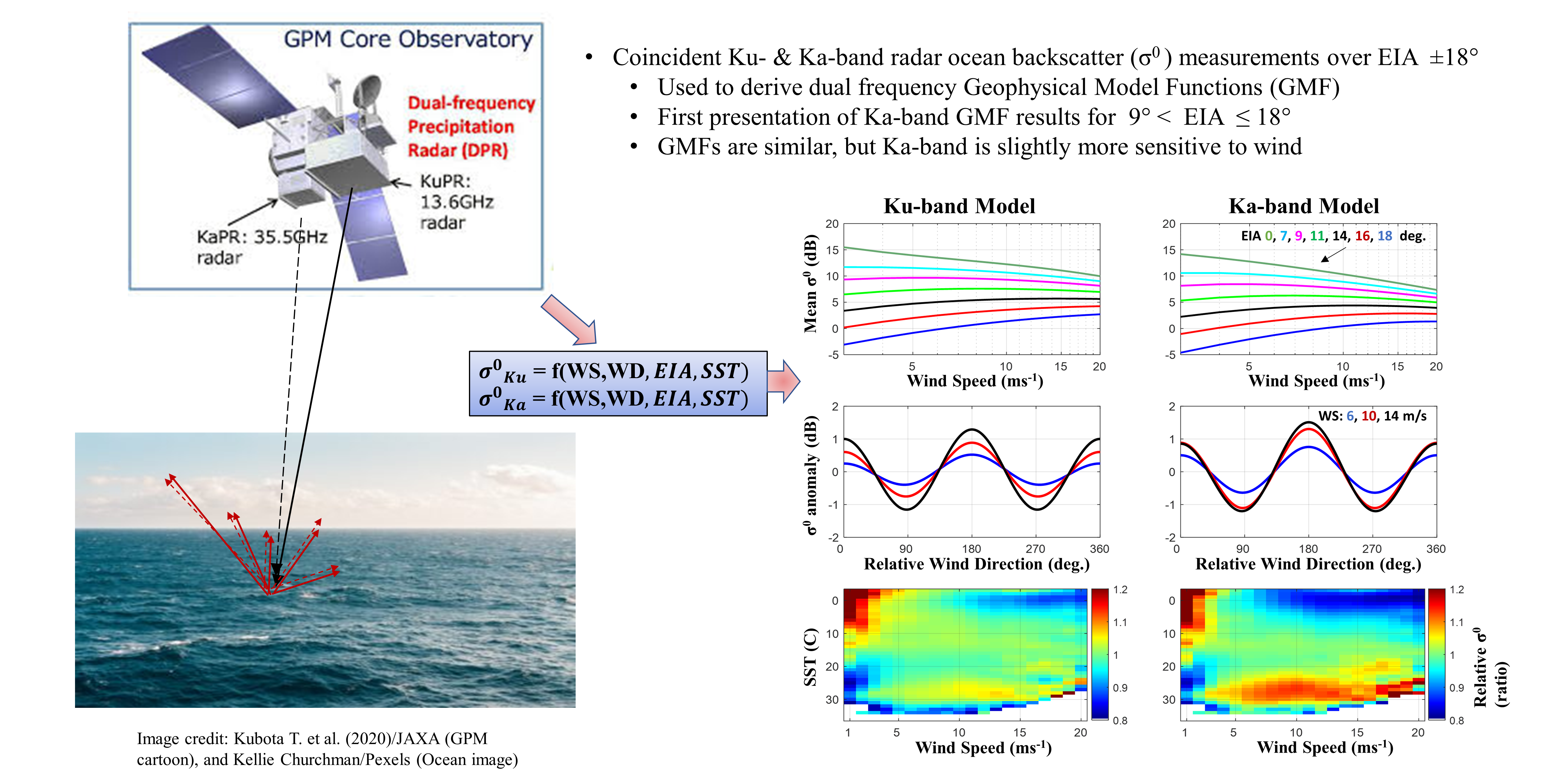
2.1. GPM Dual-Frequency Precipitation Radar (DPR)

A Ku-band (13.6 GHz, H pol) precipitation radar (KuPR) and a new Ka-band (35.5 GHz, H pol) precipitation radar (KaPR) form the dual-frequency precipitation radar (DPR) onboard the GPM core observatory as shown in Figure 1. The GPM KuPR (and TRMM PR) have an identical geometry that uses an electronically scanned phased array to scan the surface perpendicularly to the flight direction at 49 beam positions over an EIA $\pm 18°$. Contiguous beams are separated by about 0.75° in earth incidence angle, resulting a spatial footprint of about 5 km in diameter that produces a continuous 245 km measurement swath. The Ka PR also has 49 cross-track beams with the same beam width as Ku PR, but initially, only 25 of the Ka-band beams with the same range resolution as the KuPR (250 m) were overlapped with the central 25 beams of KuPR resulting in a common swath of 125 km, as shown in Figure 2a. These 25 Ka-band beams are called “matched scan (KaMS)”, and the other 24 beams which have a different range resolution (500 m) and are called “high sensitivity scan (KaHS)” because of their superior noise performance, were interleaved with the KaMS beams as shown in Figure 2a. However, on 21 May 2018, the Ka-band radar was reconfigured as shown in Figure 2b, to provide coincident measurements with KuPR over a full 245 km common swath [17]. This new configuration allows a comparison of radar backscatter characteristics at both frequencies for low EIA (nadir ± 18$°$).

2.2. GPM Microwave Imager (GMI)

The GPM Microwave Imager (GMI) is a well-calibrated, multi-channel, conical scanning total power microwave radiometer with a 931 km wide swath. It has 13 channels with frequency ranging from 10.65 to 183.31 GHz, each of which is dual-polarized (except the 23.8 GHz channel which has only V pol). A 245 km DPR swath lies at the center of the 931 km GMI swath, as shown in Figure 1, which simplifies the collocation between these two sensor measurements. Since the focus of this paper is DPR, a detailed discussion of GMI is beyond the scope of this paper, but it can be found in [20]. We used GMI wind speed (WS), and sea surface temperature (SST) retrieved by the Remote Sensing System [21]. They used intercalibrated GMI brightness temperatures (Tb) to produce ocean measurement products including WS and SST. Because the RSS GMI products are simultaneous with DPR measurements, they are expected to be more appropriate than the wind products extracted from a numerical weather forecast model.

2.3. Collocation and Quality Control

One year (2019) of Ku PR level 2 standard (2A.GPM.Ku.V8-20180723. V06A) and Ka PR experimental (2A.GPM.KaX.V8-20200326.V06X) products from the NASA GPM research data archive (https://arthurhou.pps.eosdis.nasa.gov, accessed on 15 April 2021) were used in this study. In addition to atmospheric attenuation corrected ocean surface σ⁰, the DPR product also contains navigation, sensor geometry, geolocation, and quality flags. PR rain, surface type and data quality flags were used to filter the radar backscatter to ensure rain-free ocean σ⁰ measurements, which were then smoothed (using a triangular moving average filter) to remove quantization noise caused by analog/digital conversion. Finally, the filtered ocean σ⁰ measurements were collocated with pertinent environmental parameters from two sources to provide a "match-up" dataset.

The first source of environmental parameters (WS and SST) were geophysical retrievals from coincident passive microwave GMI brightness temperatures (Tbs). These data were provided by the Remote Sensing Systems (RSS) archive (http://www.remss.com/missions/gmi/, accessed on 15 April 2021) [21] in the form of daily 0.25° earth gridded maps that were separated into ascending and descending orbit segments. For the 10 m wind speed, we used the product that was derived from low frequency channels (10.7, 18.7, 23.8, and 36.5 GHz).

The second source of environmental parameters was the European Centre for Medium-Range Weather Forecasts (ECMWF) global atmospheric reanalysis (ERA-5) [22]. Hourly 10-meter wind vector and SST products with 31 km grid spacing are available in ERA-5, which were re-gridded in 0.25° to match with GMI products.

Finally, the match-up dataset was completed by gridding the GPM DPR data (Ku and Ka) into 0.25° $\times$ 0.25° boxes, with associated GMI derived WS and SST and ERA-5 WD. All σ⁰ measurements in a box were averaged (in linear units) and boxes with a high standard deviation were discarded, and RSS data quality flags were also used to exclude any rain, sea-ice, and land contaminated data from the match-up dataset. Since DPR and GMI obtain near-simultaneous observations over a common ocean surface sub swath, the one-year time series resulted in millions of co-located, clear-sky global ocean measurements over a wide variety of environmental conditions. This provides a unique Ku/Ka σ⁰ match-up dataset that is reported for the first time in this paper. Results were produced using two environmental sets, one using GMI WS and SST with ERA-5 WD, and the other using all ERA-5 products (WS, WD, and SST). The differences were insignificant, except some mean biases (dc-offsets) between the two results. Therefore, the results with the former combination are presented in this paper.

3. Geophysical Model Function for the Ocean Ku and Ka-Band PR Backscatter

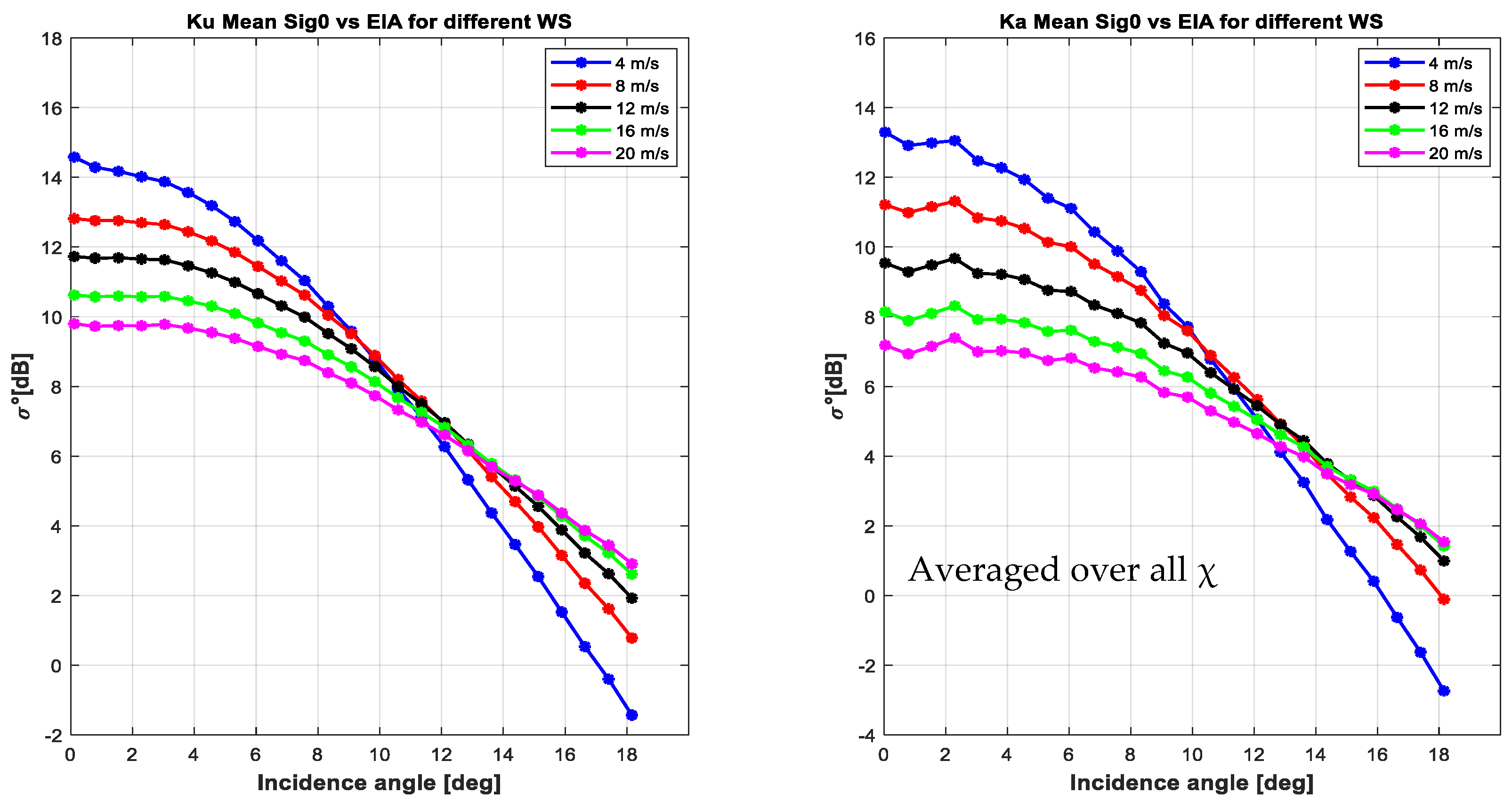
The microwave ocean surface radar backscatter (σ⁰) at the GPM DPR incidence angle range (0° to 18°) are dominated by quasi-specular scattering process, but towards the outer swath, the resonant (Bragg) scattering process also becomes significant [5]. For both regimes, the σ⁰ is directly related to the ocean surface wind vector (OVW), SST, and integral wave parameters [9,10,11,12,15,23,24]. The backscatter can be empirically modeled as a 2nd order Fourier series (higher order terms are negligible),

$$\sigma {°}_{dB}\left(f,p\right)=A_0+A_1\cos \left(\chi \right)+A_2\cos \left(2\chi \right)+B_1 \sin \left(\chi \right)+B_2 \sin \left(2\chi \right)$$

(1)

where $\sigma {°}_{dB}\left(f,p\right)$ is the sea surface normalized radar cross section at a frequency (f) and polarization (p) in dB unit. The model coefficients $A_0$, $A_1, A_2$, $B_1,$ and $B_2$ are wind speed, EIA and sea-state dependent, and χ denotes the wind direction relative to the radar azimuth look defined as χ = ${\phi }_{wind}$ − ${\phi }_{radar}$, where ${\phi }_{wind}$ is the meteorological wind direction (i.e., the direction where the wind is coming from), and ${\phi }_{radar}$ for DPR, is cross-track azimuth look (flight direction $\pm 90°$), both referring to the North. Accordingly, χ = 0 denotes the upwind specifying that the wind is blowing toward the radar look direction. Since both, Ku and Ka PR onboard GPM operate at only horizontal polarization, all references to polarization are omitted in this paper.

Historically, the radar ocean backscatter GMF has been modeled as a cosine Fourier series [25,26], but our initial analysis used both sine and cosine terms in Equation (1). However, after a comprehensive investigation, it was concluded that the sine terms were not statistically significant, and as a result, they were neglected. Figure 3 illustrates a typical comparison of the GMF, with and without the sine terms, for an EIA = 16$°$ and WS of 16 m/s. The circle symbols are the residual [$<{\sigma }^0>-A_0$] of empirical bin average $<{\sigma }^0>$, and the red solid line is the full model (Equation (1), sines and cosines) and the blue solid line is the cosine alone GMF. As shown, the contribution of the odd terms is negligible and the ${\sigma }^0$ azimuth anisotropy can be well approximated by only even terms.

$$\sigma {°}_{dB}\left(f,p\right)=A_0+A_1\cos \left(\chi \right)+A_2\cos \left(2\chi \right)$$

(2)

It should be noted that Equation (2) is the same expression used to model the ocean backscatter at moderate EIAs (20°–70°), but here, as will be depicted in the next section, the $A_1$ term is negative for EIA < 20°, which results in a reversal of upwind and downwind asymmetry, i.e., higher downwind backscatter than the upwind backscatter.

In this section, the dependence and sensitivity of Ku and Ka band σ⁰ on EIA, and the ocean surface wind speed, and wind direction are analyzed. Fourier coefficients $A_0, A_1$ and $A_2$ are derived using σ⁰ measurements for each angular beam (EIA) positions, and finally, these coefficients are modeled as a function of wind speed using polynomial fit of appropriate orders. Additionally, the SST dependence of Ku and Ka band σ⁰ is discussed. Results of sea state dependence of σ⁰ are not included in this paper; however, readers are encouraged to see [9,10,12,15] for this.

3.1. Isotropic Ku and Ka-Band ${\sigma }^0$ Model Function at Low Incidence Angles

The A₀ coefficient in Equation (1) is the azimuth independent (isotropic) σ⁰ measurement that is directly related to the wind speed (WS) for a particular earth incidence angle (EIA). Thus, it can be modeled as,

$$A_0=\sigma {°}_{dB}(\mathrm{WS}, \mathrm{EIA})$$

(3)

In order to analyze, $A_0$, the normalized radar backscatter (σ⁰) measurements of the Ku and Ka-bands were sorted in $\pm 1$ ms⁻¹ wind speed bins for each of 49 EIA beams. A conservative 3σ filter was applied to each bin to remove outliers (the 3σ values were calculated in linear, not dB, units), and any bin with less than 500 boxes was not included in the analysis. Next, using polynomial regression (in dB space), the bin average σ⁰ for each of this EIA position were expanded as a third-order polynomial of log (WS). The use of log (WS) for $A_0$ reduces the order of the polynomial fit.

$$A_0=a_{01}{x}^3+a_{02}{x}^2+a_{03}x+a_{04}$$

(4)

where x = $lo{g}_{10}\left(WS\right),$ and the numerical values of these coefficients (in dB) are given in the

Table A1. Polynomial coefficients for Ku- and Ka-band $A_0$ model in dB (Equation (4)).

Beam No	Ku					Ka
	EIA	${\mathit{a}}_{01}$	${\mathit{a}}_{02}$	${\mathit{a}}_{03}$	${\mathit{a}}_{04}$	EIA	${\mathit{a}}_{01}$	${\mathit{a}}_{02}$	${\mathit{a}}_{03}$	${\mathit{a}}_{04}$
1	18.16	0.23	−5.69	16.54	−9.71	18.16	−2.92	0.01	14.62	−11.28
2	17.41	0.70	−6.96	16.95	−8.53	17.40	−2.25	−1.64	15.01	−9.92
3	16.64	1.01	−7.82	16.97	−7.35	16.64	−1.63	−3.14	15.25	−8.62
4	15.89	1.15	−8.21	16.60	−5.99	15.88	−1.08	−4.46	15.32	−7.23
5	15.13	1.41	−8.95	16.51	−4.68	15.13	−0.51	−5.81	15.41	−6.03
6	14.38	1.69	−9.69	16.40	−3.45	14.37	0.09	−7.26	15.60	−4.79
7	13.62	1.78	−9.92	15.85	−2.12	13.61	0.69	−8.70	15.79	−3.40
8	12.86	1.73	−9.72	14.89	−0.63	12.86	1.20	−9.92	15.83	−2.20
9	12.10	1.84	−10.02	14.42	0.72	12.10	1.73	−11.21	15.93	−0.92
10	11.35	1.72	−9.64	13.33	2.14	11.35	2.21	−12.39	15.98	0.28
11	10.59	1.57	−9.12	12.12	3.55	10.59	2.67	−13.50	16.01	1.45
12	9.84	1.31	−8.34	10.70	5.07	9.84	3.04	−14.37	15.86	2.74
13	9.08	1.07	−7.55	9.27	6.51	9.08	3.46	−15.43	15.90	3.70
14	8.33	0.62	−6.23	7.41	7.98	8.33	3.83	−16.29	15.77	4.97
15	7.57	0.33	−5.25	5.81	9.42	7.57	4.03	−16.69	15.27	5.98
16	6.82	−0.11	−3.92	3.97	10.72	6.82	4.25	−17.09	14.80	6.94
17	6.06	−0.66	−2.23	1.82	12.11	6.06	4.14	−16.61	13.61	8.19
18	5.31	−1.32	−0.18	−0.66	13.57	5.31	3.95	−15.86	12.19	9.13
19	4.56	−2.07	2.12	−3.33	14.98	4.55	3.64	−14.78	10.55	10.35
20	3.80	−2.66	3.97	−5.54	16.16	3.80	3.36	−13.77	9.04	11.31
21	3.04	−3.31	5.96	−7.79	17.25	3.04	3.12	−12.93	7.77	12.03
22	2.29	−4.01	8.06	−10.05	18.14	2.29	2.79	−11.82	6.32	13.15
23	1.54	−4.73	10.28	−12.42	19.06	1.54	2.37	−10.45	4.68	13.66
24	0.79	−5.31	12.25	−14.66	19.89	0.78	2.00	−9.22	3.22	14.08
25	0.11	−6.73	17.07	−19.93	21.84	0.03	0.35	−4.06	−1.96	16.00

in Appendix A for EIA 0$°$ to 18.1$°$ (Beams 1 to 25).

The dependence of $A_0$ on WS is illustrated in Figure 4 using a log-log plot, for eight PR beam positions that include EIAs nadir to 18.1$°$. The circle symbols represent the mean value of σ⁰ measurements over all wind directions and the solid lines are their third-order polynomial fits, both in dB. At the higher EIA beam positions, σ⁰ monotonically increases with wind speed, whereas it monotonically decreases for lower EIAs near nadir. For the middle EIA beam positions, the σ⁰ dependence is not monotonic because there are two different scattering mechanisms involved. Namely, the near nadir backscatter is dominated by quasi-specular scattering that decreases σ⁰ with increased ocean roughness, but as EIA increases, Bragg scattering gradually becomes significant that increases σ⁰ with WS. These Ku results are consistent with [5,6,7,8,9,10,11,12,15], except for a small calibration bias between TRMM PR and GPM KuPR.

While these results (Figure 4) are qualitatively similar for Ka PR, there are small differences between the A₀ GMFs (Equation (4)) for Ku and Ka bands, and these differences are also a function of wind speed and incidence angle, as shown in Figure 5, which plots the differences of mean backscatter values (ΔA₀) of Ku and Ka models as a function of WS for different EIA beam positions. For the lower EIA beams, the difference increases monotonically with WS, but for the higher EIA beams, the difference first decreases with WS for lower to moderate WS, then it increases with WS for higher WS. However, for higher EIA beam positions, the differences are smaller than at lower EIA beam positions, for instance, the difference is less than 1.5 dB at EIA ~ 16$°$ for any WS between 3 and 20 m/s. Beside this, the WS sensitivity or σ⁰ gradient, defined as ($\raisebox{1ex}{$\partial {\sigma }^0$}\!\left/ \!\raisebox{-1ex}{$\partial WS$}\right.$), is shown in Figure 6 as a function of WS for the same beam positions corresponding to Figure 4. The slope of increase or decrease declines with WS at both bands. For Ka band, it declines slightly more rapidly than at Ku band for low WS region, whereas for medium to higher WS, the slopes are a little higher at Ku band. Figure 7 shows the scatter diagram of Ku and Ka PR mean σ⁰ for six fixed EIA beam positions. Symbols represent the mean σ⁰ for different wind speed bins (1 to 20 m/s at $\pm$1 m/s steps). As shown, for the outer beam positions (higher EIA), Ku and Ka PR mean σ⁰ are linearly correlated, except for higher WS, where σ⁰ become flat and start to decrease with WS. The drop of σ⁰ with increasing WS begins at relatively lower WS at the inner beam positions (lower EIA) as shown at the bottom panel of the same Figure. These correlations between Ku and Ka PR mean σ⁰ could be a useful alternative way to determine one from another, especially for outer beam positions. For example, the missing Ka outer swath for the initial phase of GPM mission (up to 22 May 2018) could be estimated from corresponding Ku band measurements. For higher WS at lower EIA, this approach would be difficult and more prone to error. However, the model derived in this paper (Equation (4)) is reliably applicable for WS 3–20 m/s for all EIA beam positions. Another important implication of Figure 7 is the variation of dynamic range of wind-roughened σ⁰ with EIA. This is shown in Figure 8, which compares the maximum wind-dependent variation of Ku band mean σ⁰ with that at Ka band. As shown, although both have similar dynamic ranges for EIA ~> 9$°$, Ka band mean σ⁰ has higher dynamic range for EIA < 9$°$.

Finally, the mean values of binned average σ⁰ for Ku and Ka bands are shown in Figure 9 as a function of EIA for different wind speeds. The σ⁰ monotonically decreases with increasing incidence angle from nadir to 18.2°. Additionally, the σ⁰ decreases monotonically with wind speed at EIAs near nadir, but σ⁰ increases monotonically with wind speed near EIA 18.2°, with a transition in the middle where σ⁰ becomes relatively insensitive to WS (for WS $\ge 4$ ms⁻¹). For KuPR, this transition occurs over EIA 11°–13$°$, whereas for KaPR it occurs over EIA 12°–14°. Additionally, these transition regions vary with the relative azimuth look, for upwind/downwind/crosswind directions, as shown for KuPR in Figure 10 (these variations are proportionately similar at Ka-band which is not shown here). This EIA range of reduced σ⁰ variability is useful for the radar inter-calibration between these kinds of instruments [5]. Therefore, based upon these results, we conclude that the two GMF’s are similar and are applicable for a WS range of 3–20 ms⁻¹ and for all EIA beam positions.

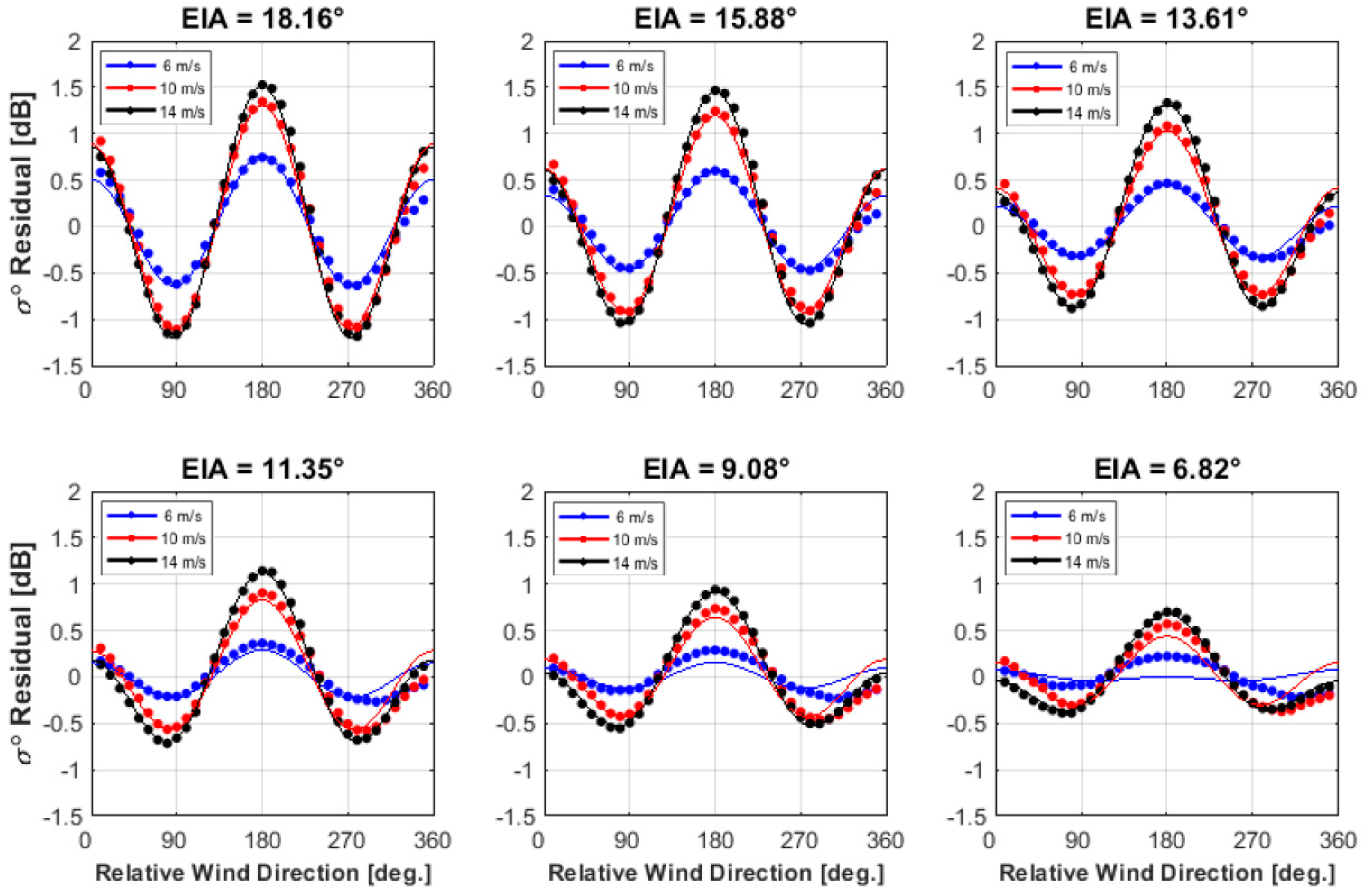
3.2. σ⁰ Azimuthal Anisotropy

The directional anisotropy of ocean surface σ⁰ is a function of WS, relative wind direction, and EIA. We can separate the directional signal of σ⁰ (in dB) by computing the residual of σ⁰ as follows,

$${\sigma }^0-A_0={\sigma }^0{}_{\left(residual\right)}=A_1 \cos \left(\chi \right)+A_2 \cos \left(2\chi \right)$$

(5)

To analyze the directional anisotropy of both KuPR and KaPR, in accordance with Equation (5), the σ⁰ measurements in WS bins (±1 m/s) were further sorted into 10$°$ relative wind direction (χ) bins. Afterwards, the Fourier series approximation of Equation (2) was applied to the bin average of both Ku and Ka PR ${\sigma }^0$ (in dB space), to derive $A_1$ and $A_2$ coefficients for each WS and EIA bin position. Finally, $A_1$ and $A_2$ Fourier coefficients, thus derived, were modeled as a function of WS using third and seventh order polynomial regressions (in dB space), respectively. Unlike the case of $A_0$ in Equation (4), use of log (WS) for $A_1$ and $A_1$ does not reduce the order of the polynomials, thus WS measurements in linear units were used in these cases.

$$A_1=a_{11}{u}^3+a_{12}{u}^2+a_{13}u+a_{14}$$

(6)

and,

$$A_2=a_{21}{u}^7+a_{22}{u}^6+a_{23}{u}^5+a_{24}{u}^4+a_{25}{u}^3+a_{26}{u}^2+a_{27}u+a_{28}$$

(7)

where $u=WS$, and the values of the polynomial coefficients $a_{11}$ through $a_{14}$ and $a_{21}$ through $a_{28}$ (in dB) are given in the

Table A2. Polynomial coefficients for Ku- and Ka-band $A_1$ model in dB (Equation (6)).

Beam No	Ku					Ka
	EIA	${\mathit{a}}_{11}$	${\mathit{a}}_{12}$	${\mathit{a}}_{13}$	${\mathit{a}}_{14}$	EIA	${\mathit{a}}_{11}$	${\mathit{a}}_{12}$	${\mathit{a}}_{13}$	${\mathit{a}}_{14}$
1	18.16	−0.0001	0.0023	−0.0243	−0.0576	18.16	0.0002	−0.0072	0.0545	−0.2377
2	17.41	0.0000	0.0011	−0.0160	−0.0694	17.4	0.0002	−0.0072	0.0458	−0.1950
3	16.64	0.0000	0.0002	−0.0132	−0.0550	16.64	0.0002	−0.0062	0.0264	−0.1137
4	15.89	0.0001	−0.0013	−0.0043	−0.0476	15.88	0.0002	−0.0054	0.0105	−0.0432
5	15.13	0.0001	−0.0017	−0.0039	−0.0363	15.13	0.0003	−0.0071	0.0214	−0.0561
6	14.38	0.0001	−0.0029	0.0048	−0.0437	14.37	0.0003	−0.0073	0.0202	−0.0352
7	13.62	0.0001	−0.0043	0.0163	−0.0650	13.61	0.0003	−0.0085	0.0280	−0.0408
8	12.86	0.0002	−0.0047	0.0192	−0.0664	12.86	0.0003	−0.0090	0.0308	−0.0351
9	12.1	0.0002	−0.0056	0.0260	−0.0751	12.1	0.0004	−0.0103	0.0450	−0.0640
10	11.35	0.0002	−0.0066	0.0356	−0.0916	11.35	0.0004	−0.0116	0.0583	−0.0891
11	10.59	0.0002	−0.0061	0.0315	−0.0780	10.59	0.0004	−0.0134	0.0768	−0.1253
12	9.84	0.0002	−0.0068	0.0398	−0.1047	9.84	0.0005	−0.0155	0.0999	−0.1827
13	9.08	0.0003	−0.0086	0.0572	−0.1425	9.08	0.0005	−0.0152	0.0990	−0.1842
14	8.33	0.0003	−0.0088	0.0616	−0.1510	8.33	0.0005	−0.0161	0.1110	−0.2023
15	7.57	0.0003	−0.0111	0.0850	−0.1987	7.57	0.0005	−0.0152	0.1059	−0.1826
16	6.82	0.0003	−0.0108	0.0836	−0.1942	6.82	0.0005	−0.0170	0.1249	−0.2141
17	6.06	0.0003	−0.0109	0.0872	−0.2043	6.06	0.0005	−0.0165	0.1229	−0.1963
18	5.31	0.0003	−0.0105	0.0854	−0.1900	5.31	0.0005	−0.0163	0.1255	−0.1987
19	4.56	0.0003	−0.0091	0.0722	−0.1562	4.55	0.0005	−0.0148	0.1125	−0.1371
20	3.8	0.0003	−0.0079	0.0584	−0.0945	3.8	0.0004	−0.0127	0.0952	−0.0876
21	3.04	0.0001	−0.0040	0.0254	−0.0119	3.04	0.0004	−0.0131	0.1065	−0.1298
22	2.29	0.0002	−0.0087	0.0932	−0.2913	2.29	0.0004	−0.0143	0.1291	−0.2344
23	1.54	0.0003	−0.0091	0.0944	−0.2678	1.54	0.0004	−0.0148	0.1487	−0.3375
24	0.79	0.0001	−0.0053	0.0574	−0.1468	0.78	0.0004	−0.0147	0.1507	−0.3238
25	0.11	−0.0001	0.0045	−0.0434	0.1710	0.03	0.0004	−0.0141	0.1347	−0.2774

,

Table A3. Polynomial coefficients for Ku-band $A_2$ model in dB (Equation (7)).

Beam No	EIA	${\mathit{a}}_{21}$	${\mathit{a}}_{22}$	${\mathit{a}}_{23}$	${\mathit{a}}_{24}$	${\mathit{a}}_{25}$	${\mathit{a}}_{26}$	${\mathit{a}}_{27}$	${\mathit{a}}_{28}$
1	18.16	−2.51 × 10−8	1.37 × 10−6	−1.89 × 10−5	−0.00013	0.00321	0.019326	−0.38819	1.591838
2	17.41	−3.03 × 10−8	1.88 × 10−6	−3.86 × 10−5	0.000258	−0.00098	0.042961	−0.45597	1.628328
3	16.64	−1.13 × 10−7	8.54 × 10−6	−0.00026	0.004169	−0.04013	0.263471	−1.10123	2.343184
4	15.89	−1.21 × 10−7	9.35 × 10−6	−0.00029	0.004749	−0.04628	0.298097	−1.19719	2.406955
5	15.13	−7.46 × 10−8	5.58 × 10−6	−0.00017	0.002561	−0.0242	0.169838	−0.80344	1.891615
6	14.38	−7.61 × 10−8	5.73 × 10−6	−0.00017	0.002692	−0.0255	0.174281	−0.79615	1.810658
7	13.62	−4.49 × 10−8	3.22 × 10−6	−8.98 × 10−5	0.00127	−0.01147	0.094093	−0.54922	1.46773
8	12.86	−5.94 × 10−8	4.41 × 10−6	−0.00013	0.001983	−0.01855	0.131392	−0.64059	1.510883
9	12.1	−4.93 × 10−8	3.60 × 10−6	−0.0001	0.001547	−0.01442	0.107759	−0.56267	1.376621
10	11.35	−3.84 × 10−8	2.83 × 10−6	−8.28 × 10−5	0.001264	−0.01231	0.097383	−0.52466	1.287835
11	10.59	−5.38 × 10−8	4.02 × 10−6	−0.00012	0.001938	−0.01902	0.133029	−0.61068	1.328016
12	9.84	−6.36 × 10−8	4.95 × 10−6	−0.00016	0.002595	−0.02585	0.170093	−0.70143	1.37417
13	9.08	−4.43 × 10−8	3.27 × 10−6	−9.63 × 10−5	0.001497	−0.01446	0.103187	−0.49284	1.091061
14	8.33	−2.86 × 10−8	2.02 × 10−6	−5.61 × 10−5	0.000817	−0.0079	0.065707	−0.37112	0.906196
15	7.57	−2.23 × 10−8	1.15 × 10−6	−1.53 × 10−5	−9.89E−05	0.00298	−0.00386	−0.14594	0.599584
16	6.82	−7.29 × 10−8	4.99 × 10−6	−0.00013	0.001829	−0.0146	0.084527	−0.36466	0.780318
17	6.06	−8.53 × 10−8	6.10 × 10−6	−0.00017	0.002612	−0.02305	0.133651	−0.49913	0.888727
18	5.31	−1.31 × 10−7	9.80 × 10−6	−0.0003	0.004725	−0.04346	0.241628	−0.77882	1.139603
19	4.56	−2.51 × 10−7	1.94 × 10−5	−0.00061	0.01013	−0.09551	0.518007	−1.50914	1.848456
20	3.8	−2.91 × 10−7	2.16 × 10−5	−0.00065	0.010106	−0.08874	0.441954	−1.16733	1.286324
21	3.04	−4.20 × 10−7	3.08 × 10−5	−0.0009	0.013482	−0.10939	0.470893	−0.95257	0.640136
22	2.29	−1.11 × 10−8	−1.13 × 10−5	0.000112	−0.00337	0.048202	−0.35222	1.258894	−1.70139
23	1.54	−3.55 × 10−7	2.67 × 10−5	−0.00082	0.013007	−0.11706	0.596926	−1.60916	1.813668
24	0.79	−1.29 × 10−7	8.34 × 10−5	−0.0002	0.002153	−0.00725	−0.03711	0.326281	−0.60025
25	0.11	2.79 × 10−7	−2.34 × 10−5	0.000803	−0.0144	0.144452	−0.79752	2.20042	−2.32417

, and

Table A4. Polynomial coefficients for Ka-band $A_2$ model in dB (Equation (7)).

Beam No	EIA	${\mathit{a}}_{21}$	${\mathit{a}}_{22}$	${\mathit{a}}_{23}$	${\mathit{a}}_{24}$	${\mathit{a}}_{25}$	${\mathit{a}}_{26}$	${\mathit{a}}_{27}$	${\mathit{a}}_{28}$
1	18.16	2.42 × 10−7	−1.95 × 10−5	0.000630	−0.010285	0.086533	−0.327061	0.300739	1.182616
2	17.4	2.24 × 10−7	−1.81 × 10−5	0.000584	−0.009520	0.079453	−0.290412	0.197955	1.253774
3	16.64	1.64 × 10−7	−1.33 × 10−5	0.000430	−0.006907	0.054482	−0.155678	−0.187766	1.661966
4	15.88	1.64 × 10−7	−1.35 × 10−5	0.000440	−0.007202	0.058886	−0.190922	−0.049940	1.412138
5	15.13	1.77 × 10−7	−1.46 × 10−5	0.000483	−0.008099	0.069775	−0.266707	0.221679	0.986715
6	14.37	1.88 × 10−7	−1.56 × 10−5	0.000520	−0.008830	0.078501	−0.327420	0.441136	0.634368
7	13.61	2.07 × 10−7	−1.72 × 10−5	0.000577	−0.009927	0.090532	−0.402978	0.686282	0.284689
8	12.86	2.00 × 10−7	−1.66 × 10−5	0.000560	−0.009654	0.088519	−0.398082	0.695758	0.208310
9	12.1	1.84 × 10−7	−1.55 × 10−5	0.000527	−0.009213	0.085757	−0.394888	0.730148	0.078091
10	11.35	2.21 × 10−7	−1.85 × 10−5	0.000628	−0.010983	0.103633	−0.497933	1.038398	−0.317011
11	10.59	1.88 × 10−7	−1.59 × 10−5	0.000545	−0.009590	0.090552	−0.430458	0.863195	−0.171659
12	9.84	1.75 × 10−7	−1.51 × 10−5	0.000530	−0.009536	0.092273	−0.453516	0.966268	−0.354499
13	9.08	1.93 × 10−7	−1.63 × 10−5	0.000558	−0.009872	0.094156	−0.458488	0.974761	−0.398545
14	8.33	1.83 × 10−7	−1.56 × 10−5	0.000540	−0.009598	0.091517	−0.442654	0.922165	−0.358762
15	7.57	1.86 × 10−7	−1.58 × 10−5	0.000540	−0.009504	0.089661	−0.428214	0.873555	−0.330738
16	6.82	1.33 × 10−7	−1.14 × 10−5	0.000390	−0.006815	0.062436	−0.274513	0.433755	0.121128
17	6.06	6.59 × 10−8	−5.83 × 10−6	0.000203	−0.003484	0.029146	−0.091183	−0.069137	0.611545
18	5.31	−5.98 × 10−8	4.23 × 10−6	−0.000126	0.002153	−0.024887	0.192571	−0.805417	1.298094
19	4.55	−1.88 × 10−7	1.43 × 10−5	−0.000445	0.007450	−0.073550	0.434311	−1.379665	1.725746
20	3.8	−2.29 × 10−7	1.76 × 10−5	−0.000545	0.008844	−0.081123	0.420976	−1.104958	1.037734
21	3.04	−5.07 × 10−8	1.79 × 10−6	0.000033	−0.002468	0.045852	−0.391507	1.617923	−2.622437
22	2.29	−3.10 × 10−7	2.39 × 10−5	−0.000747	0.012150	−0.110696	0.558874	−1.391901	1.206958
23	1.54	9.61 × 10−8	−1.01 × 10−5	0.000419	−0.008970	0.106483	−0.701081	2.392505	−3.269356
24	0.78	−2.32 × 10−7	1.82 × 10−5	−0.000592	0.010423	−0.108244	0.664801	−2.196144	2.936393
25	0.03	2.58 × 10−6	−0.000205	0.006542	−0.107272	0.958791	−4.604580	11.119489	−10.804452

in Appendix A for EIA 0$°$ to 18.1$°$ (Beams 1 to 25).

The $A_1$ and $A_2$ coefficients, for the corresponding EIA beam positions, are shown as a function of WS in Figure 11 and Figure 12, respectively. Symbols in both Figures represent the Fourier coefficients found from Equation (2), and the solid lines represent the corresponding polynomial fits (Equations (6) and (7)). For both bands, $A_1$ is negative, and the magnitude becomes more negative with increasing WS. Additionally, for the same EIA, the magnitude of the Ka band $A_1$ is slightly more negative, and the doubling of this coefficient is the measure of upwind-down wind asymmetry. For the $A_2$ coefficient, both bands have similar patterns, which decrease with increasing WS and reach a minimum (at ~6 m/s (Ku) and ~5 m/s (Ka)). Afterwards, the magnitude of $A_2$ rapidly increases with WS until it approximately saturates at WS ~= 14 m/s for Ku band and WS ~= 12 m/s for Ka band. The $A_2$ coefficient is a measure of upwind–crosswind asymmetry or total directional anisotropy, and it increases with EIA.

The residual (anomaly) of the KuPR σ⁰ is presented in Figure 13 as a function of relative wind direction for selected EIAs and WS. The symbols are the residual of the measured bin average, and the solid lines are the corresponding model (Equation (5)). As shown, the bi-harmonic directional signal increases with both WS and EIA, and the model is in excellent agreement with the empirical measurements for all cases, except for the 6.8° EIA (and less), which is slightly degraded for relative WD: 270°–360°, especially for lower WS cases. The corresponding results for KaPR are presented in Figure 14, but for these cases the quality of the model fit is somewhat lacking for the lower three EIAs. For these cases, the model downwind response (relative WD = 180°) is progressively underestimated (at the 0.1 dB level), and the model fit with the empirical measurements for relative WD of 270°–360° disagree at the 0.2 dB level. Since both the Ku and Ka models have issues with this same relative WD range, the empirical measurements are suspect. Further, the model has an even symmetry with relative WD, whereas the empirical measurements have not. The reason for this anomaly is not understood, but given the low EIA, one possible explanation is the effect of ocean wave swell, which has not been considered in this analysis.

The relative difference between the Ku and Ka band σ⁰ directional residual (${\sigma }_{Ku-residual}^0\left[dB\right]-{\sigma }_{Ka-residual}^0\left[dB\right]$), is given in Figure 15 as a function of relative wind direction for the WS averaged over 6–14 m/s at different EIAs. As shown, the maximum difference occurs at the upwind, downwind and crosswind directions which is also a function of the EIA. Now consider the delta-σ⁰ residual, calculated at upwind, downwind and crosswind for an EIA ~ 16°, as a function of WS (given in Figure 16). At the downwind direction, the KaPR has a higher wind direction signal than KuPR for all WS, whereas for the upwind and crosswind, the polarity of the difference depends on WS range.

3.2.1. Upwind and Downwind Asymmetry of σ⁰

One of the interesting features of the σ⁰ WD anisotropy at low EIA is that it has an opposite upwind/downwind asymmetry compared to the conventional scatterometers that operate at moderate incidence angles (20°–70°). As shown in Figure 13 and Figure 14, DPR measures a higher σ⁰ from the downwind direction than that from the upwind direction, and 2$A_1$ is the measure of the peak-to-peak upwind/downwind asymmetry. The differences between downwind and upwind σ⁰ measurements, separately for both KuPR and KaPR as a function of WS: 3–20 m/s, are shown in Figure 17 for six different EIAs: 6.8°–18.2°, and it is noted that for all EIAs, the measured σ⁰ asymmetry increases with WS of 6–16 m/s. Chu et al. (2012) [12] also presented similar results for TRMM KuPR and Mouche et al. (2006) [27] reported the same trends of asymmetries for a C band radar at low incidence angle. However, this paper presents new information concerning a higher upwind/downwind asymmetry for Ka band compared to the Ku band. For example, at EIA ~ 12°, the Ku band asymmetry is about 0.7 dB for a WS of 16 m/s, while it is > 1 dB for Ka band for the same EIA and WS.

3.2.2. Downwind and Crosswind Anisotropy of σ⁰

For scatterometers operating at moderate EIAs, the $A_2$ coefficient in Equations (2) and (5), usually defines the peak-to-peak (upwind to crosswind) anisotropy of σ⁰. However, for this low EIA range, since $A_1$ is negative and not negligible, backscatter response at the downwind direction is the sum of $A_1$ and $A_2$. Therefore, the peak-to-peak anisotropy for this EIA range is defined downwind to crosswind which is > 2$A_2$. Figure 18 shows the peak-to-peak σ⁰ anisotropy for Ku and Ka bands, as a function of WS for different EIAs. Additionally, Figure 19 shows the same results as a function of EIA for WS: 6–18 m/s. As previously discussed, the shape of this curve follows that of the A₂ coefficient for both WS and EIA.

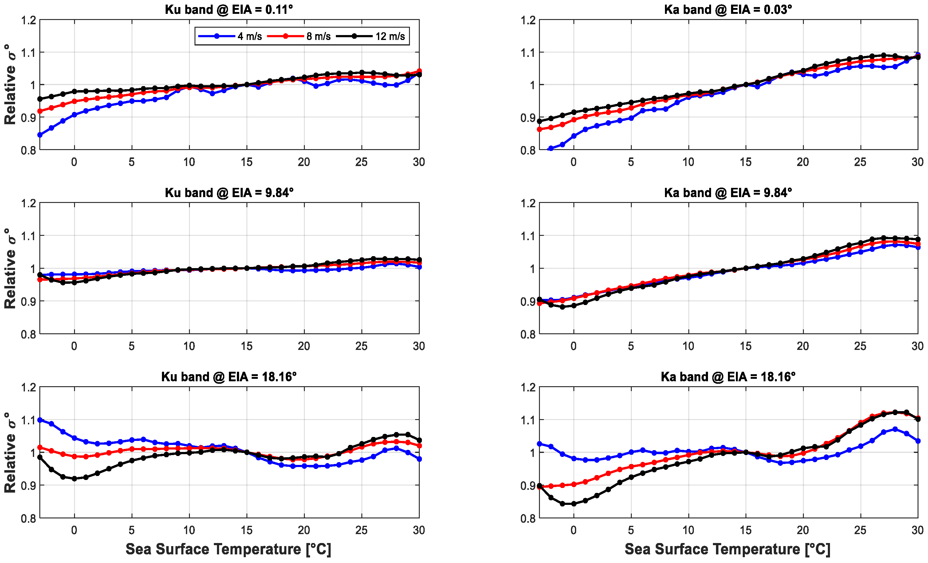
3.3. SST Dependency of σ⁰

In previous research [18], it was concluded that the SST has a small but significant effect on the observed ocean σ⁰ at Ku band; but in this paper, these SST effects were not explicitly identified in the development of the three dimensional (3D) GMF = f(WS, WD, EIA) Ku- and Ka-bands. Unfortunately, the available σ⁰ match-up datasets have insufficient observations for the development of a 4D GMF = f(WS, WD, SST, EIA); however, a somewhat qualitative assessment of the impact of SST on in the GMFs are presented below.

At low microwave frequencies (1–8 GHz), sea surface temperature affects the dielectric constant of sea water and the resulting Fresnel reflection coefficient; however, at Ku and Ka bands this effect is weak [24]. On the other hand, SST also affects the surface tension and viscosity of the sea water, both of which control the amplitude of the capillary wave spectral region of the sea surface roughness. For the low wind speed regime (~WS < 6m/s), surface tension dominates the capillary wave spectrum; whereas for higher WS, wave breaking occurs and viscosity then plays a significant role in controlling the roughness. Thus, surface tension and viscosity, which tend to reduce surface roughness, both decrease with increasing SST. As a result, ocean σ⁰ increases with SST, and V-polarized signals exhibit larger dependencies on SST than H-pol signals [18]. Since GPM DPR measurements are both H pol, this paper presents only SST impacts on H pol at low incidence angles.

Thus, the dependence of σ⁰ on SST was empirically characterized for both Ku- and Ka-bands as a function of EIA, WS and WD, using the following statistical procedure. For the EIA investigation, the σ⁰ values, in linear power ratio units, were bin averaged (over all WS and WD) in 1 °C steps of SST 0–30 °C. Next, the binned averages were normalized to the corresponding σ⁰ values at 15 C, and results presented in Figure 20 show that there is an approximately linear dependence of the relative σ⁰ on SST that is independent of EIA beam positions at both frequencies. However, as expected, the SST dependency is significantly stronger (> 2 x slope) for Ka band. For example, for an EIA = 9°, the overall variation of mean σ⁰ with SST over the range 0–30 °C is < ± 5% at Ku, whereas it is > ± 10% for Ka.

Next, these SST binned normalized σ⁰ data were sorted and averaged (separately for Ku and Ka) over WS values of 4, 8 and 12 m/s ranges, and the results are presented in Figure 21 for EIAs of 0.1°, 9.8° and 18.6°. Here, the results are similar to Figure 20 (averaged over all WS); however, there is also a slight WS dependence as noted by the separation of the curves. This is especially notable at the higher EIA that we suspect may be attributed to the WD effects presented next.

Next, changes in the GMF relative wind direction response due to SST were assessed using σ⁰ data (not normalized), but here only the outer most beam position (EIA = 18°) was selected since it has the largest anisotropy. The results are shown in Figure 22 for SST of 5 and 25 °C as a function of relative WD for WS values of 8, 10 and 12 m/s. For Ku-band, there appears to be no SST effects and the relative WD patterns are essentially identical; on the other hand, at Ka-band the effect is small but significant. It appears that the σ⁰ WD pattern is unchanged except for a small increase in the mean (dc offset), which is consistent with the observation presented in Figure 20.

Finally, the SST impacts, on the mean value of KuPR and KaPR σ⁰, are presented in Figure 23 as in set of 2D images for observed ranges of SST and WS. The color scale represents the mean σ⁰ relative to corresponding σ⁰ at 15 °C. As shown, for WS ~> 5 m/s, the mean backscatter at both band increases with SST; however, the contrast is significantly higher at Ka-band. For WS ~< 5 m/s, the trend is opposite at both bands. These SST dependent relative weights can be used as a correction factor to account for the SST impacts on the GMF. One such approach was used by [28] to correct and validate NSCAT-5 GMF. For the DPR model of this paper (Equation (2)), this can be implemented as follows,

$${\sigma }_{corrected}^0\left(f\right)=\mathrm{W}\left(\mathrm{SST},\mathrm{WS}\right) x {\sigma }_{linear}^0\left(f\right)$$

(8)

where ${\sigma }_{linear}^0\left(f\right)$ is σ⁰ model in linear scale, and W is SST-impact correction factor which can determined from the tables such as presented in Figure 23 for different EIA beam positions. Sample correction factors, $\mathrm{W}\left(\mathrm{SST},\mathrm{WS}\right),$ for Ku- and Ka-band models at EIA = 18° are given in the

Table A5. SST correction factor (W) for Ku-band model for EIA = 18° in linear unit (Equation (8)). The bins with inadequate observations are shown as not-a-number (NaN).

SST (C)	WS (m/s)
	1	2	3	4	5	6	7	7	9	10	11	12	13	14	15	16	17	18	19	20
−3	NaN	1.31	1.15	1.10	1.07	1.04	1.02	1.01	1.00	0.99	0.98	0.98	0.98	1.01	1.01	1.00	0.98	0.95	0.93	0.88
−2	NaN	1.28	1.17	1.09	1.05	1.03	1.02	1.00	0.99	0.97	0.95	0.95	0.94	0.95	0.95	0.93	0.92	0.91	0.91	0.88
−1	NaN	1.20	1.12	1.06	1.04	1.02	1.01	0.99	0.98	0.96	0.94	0.93	0.91	0.91	0.91	0.89	0.88	0.88	0.88	0.86
0	1.26	1.15	1.08	1.04	1.03	1.02	1.00	0.99	0.97	0.95	0.94	0.92	0.91	0.91	0.90	0.88	0.88	0.88	0.89	0.87
1	1.25	1.15	1.07	1.03	1.02	1.01	1.00	0.99	0.97	0.95	0.94	0.92	0.92	0.92	0.91	0.90	0.89	0.90	0.91	0.89
2	1.24	1.14	1.06	1.03	1.02	1.01	1.00	0.99	0.98	0.97	0.95	0.94	0.93	0.93	0.93	0.92	0.92	0.92	0.93	0.91
3	1.20	1.12	1.06	1.03	1.02	1.02	1.01	1.00	0.99	0.98	0.97	0.95	0.94	0.94	0.94	0.94	0.94	0.94	0.95	0.93
4	1.20	1.13	1.06	1.03	1.03	1.02	1.01	1.00	1.00	1.00	0.98	0.96	0.96	0.96	0.96	0.95	0.95	0.95	0.96	0.95
5	1.21	1.13	1.06	1.04	1.03	1.03	1.02	1.01	1.01	1.00	0.99	0.97	0.97	0.97	0.97	0.97	0.96	0.96	0.95	0.94
6	1.18	1.14	1.07	1.04	1.03	1.03	1.02	1.01	1.01	1.00	0.99	0.98	0.98	0.98	0.98	0.98	0.98	0.97	0.96	0.94
7	1.13	1.14	1.07	1.03	1.02	1.02	1.01	1.01	1.01	1.01	1.00	0.99	0.99	0.99	0.99	0.99	0.99	0.98	0.98	0.96
8	1.11	1.12	1.06	1.03	1.02	1.01	1.01	1.01	1.01	1.01	1.00	0.99	0.99	1.00	0.99	0.99	0.99	0.98	0.99	0.98
9	1.06	1.10	1.06	1.03	1.02	1.01	1.01	1.01	1.01	1.01	1.01	1.00	0.99	1.00	1.00	0.99	0.99	0.99	1.00	0.99
10	1.04	1.07	1.05	1.02	1.01	1.01	1.01	1.01	1.02	1.01	1.01	1.00	1.00	1.00	1.00	1.00	0.99	0.99	1.00	0.98
11	1.02	1.05	1.03	1.01	1.01	1.01	1.01	1.01	1.02	1.01	1.01	1.00	1.00	1.01	1.01	1.00	0.99	0.98	0.98	0.97
12	1.03	1.05	1.03	1.02	1.01	1.01	1.01	1.01	1.02	1.02	1.01	1.01	1.01	1.01	1.01	1.00	0.99	0.98	0.98	0.97
13	1.07	1.05	1.03	1.02	1.01	1.01	1.01	1.01	1.01	1.02	1.01	1.01	1.01	1.01	1.01	1.01	1.01	1.00	1.00	0.98
14	1.05	1.03	1.01	1.01	1.01	1.01	1.01	1.01	1.01	1.01	1.01	1.00	1.00	1.01	1.01	1.02	1.01	1.00	1.00	0.99
15	1.00	1.00	1.00	1.00	1.00	1.00	1.00	1.00	1.00	1.00	1.00	1.00	1.00	1.00	1.00	1.00	1.00	1.00	1.00	1.00
16	1.01	0.98	0.98	0.98	0.99	0.99	0.99	0.99	0.99	0.99	0.99	0.99	0.99	1.00	1.00	1.00	1.00	1.00	1.01	1.00
17	1.03	0.96	0.97	0.97	0.98	0.99	0.99	0.99	0.99	0.99	0.99	0.98	0.99	1.01	1.01	1.00	1.00	0.99	0.99	0.98
18	1.00	0.95	0.95	0.96	0.97	0.98	0.98	0.98	0.98	0.98	0.98	0.98	0.99	1.00	1.01	0.99	1.01	1.01	1.00	0.98
19	0.98	0.94	0.94	0.96	0.97	0.98	0.98	0.98	0.98	0.98	0.98	0.98	0.98	1.00	1.00	1.01	1.03	1.02	1.01	0.99
20	0.95	0.91	0.94	0.96	0.97	0.98	0.98	0.98	0.98	0.98	0.98	0.99	0.99	1.00	1.01	1.03	1.03	1.02	1.00	0.93
21	0.91	0.90	0.93	0.96	0.97	0.98	0.98	0.98	0.99	0.99	0.99	0.99	1.00	1.01	1.01	1.03	1.02	1.02	1.01	0.93
22	0.88	0.90	0.94	0.96	0.97	0.98	0.99	0.99	0.99	1.00	0.99	0.99	0.99	1.00	1.01	1.00	1.00	1.02	1.02	0.97
23	0.87	0.89	0.93	0.96	0.98	0.99	0.99	1.00	1.00	1.01	1.00	1.00	0.99	0.99	1.00	0.98	0.97	0.98	1.00	0.99
24	0.83	0.87	0.93	0.97	0.98	0.99	1.00	1.00	1.01	1.02	1.02	1.01	1.01	1.00	1.00	0.97	0.93	0.96	1.02	1.08
25	0.81	0.87	0.94	0.98	0.99	1.00	1.01	1.02	1.02	1.04	1.03	1.03	1.02	1.01	1.01	1.00	0.97	1.00	1.06	1.09
26	0.84	0.90	0.95	0.99	1.01	1.01	1.02	1.03	1.03	1.05	1.05	1.04	1.03	1.03	1.03	1.03	1.04	1.04	1.00	0.90
27	0.86	0.92	0.98	1.01	1.01	1.02	1.03	1.03	1.04	1.05	1.05	1.05	1.05	1.05	1.02	1.02	1.03	1.00	0.98	0.87
28	0.89	0.96	1.01	1.01	1.02	1.03	1.03	1.03	1.04	1.04	1.05	1.05	1.07	1.05	1.02	1.01	1.05	1.05	1.22	NaN
29	0.90	0.97	1.00	1.00	1.01	1.02	1.03	1.03	1.03	1.03	1.04	1.05	1.06	1.06	1.04	1.03	1.01	1.27	NaN	NaN
30	0.87	0.94	0.97	0.98	1.00	1.01	1.02	1.02	1.02	1.02	1.02	1.04	1.03	1.03	1.04	1.04	0.95	NaN	NaN	NaN
31	0.81	0.88	0.92	0.95	0.98	1.00	1.00	1.00	0.99	0.99	0.98	0.98	0.97	0.92	0.94	0.90	0.79	NaN	NaN	NaN
32	0.66	0.75	0.82	0.89	0.94	0.96	0.95	0.95	0.94	0.95	0.93	0.94	0.92	0.85	0.88	NaN	NaN	NaN	NaN	NaN
33	0.50	0.69	0.82	0.85	0.91	0.94	0.92	0.88	0.88	0.91	0.87	0.94	0.83	NaN	NaN	NaN	NaN	NaN	NaN	NaN
34	0.42	0.96	0.93	0.87	0.94	0.90	0.89	0.89	0.92	0.88	0.82	0.99	NaN	NaN	NaN	NaN	NaN	NaN	NaN	NaN

and

Table A6. SST correction factor (W) for Ka-band model for EIA = 18° in linear unit (Equation (8)). The bins with inadequate observations are shown as not-a-number (NaN).

SST (C)	WS (m/s)
	1	2	3	4	5	6	7	7	9	10	11	12	13	14	15	16	17	18	19	20
−3	NaN	1.25	1.08	1.03	0.99	0.95	0.92	0.89	0.88	0.88	0.89	0.90	0.90	0.92	0.92	0.92	0.90	0.88	0.86	0.82
−2	NaN	1.22	1.11	1.02	0.97	0.94	0.92	0.90	0.88	0.87	0.86	0.86	0.86	0.87	0.87	0.86	0.85	0.84	0.84	0.82
−1	NaN	1.13	1.06	0.99	0.96	0.94	0.92	0.90	0.88	0.86	0.85	0.84	0.84	0.84	0.84	0.83	0.82	0.81	0.81	0.81
0	1.28	1.10	1.02	0.98	0.96	0.95	0.92	0.90	0.88	0.87	0.85	0.84	0.84	0.84	0.84	0.83	0.82	0.82	0.83	0.81
1	1.28	1.11	1.02	0.98	0.96	0.95	0.93	0.91	0.89	0.88	0.86	0.85	0.85	0.85	0.85	0.84	0.84	0.85	0.85	0.83
2	1.28	1.10	1.02	0.98	0.96	0.95	0.94	0.92	0.91	0.90	0.88	0.87	0.86	0.87	0.87	0.86	0.86	0.87	0.87	0.85
3	1.24	1.09	1.02	0.98	0.97	0.97	0.95	0.94	0.93	0.92	0.90	0.89	0.88	0.89	0.89	0.89	0.89	0.89	0.90	0.88
4	1.25	1.11	1.03	0.99	0.98	0.98	0.96	0.95	0.94	0.94	0.92	0.91	0.90	0.91	0.91	0.91	0.91	0.91	0.91	0.90
5	1.27	1.11	1.04	1.00	0.99	0.98	0.97	0.96	0.95	0.95	0.93	0.92	0.92	0.92	0.93	0.93	0.92	0.91	0.90	0.89
6	1.23	1.12	1.05	1.01	0.99	0.99	0.97	0.96	0.96	0.96	0.95	0.94	0.94	0.94	0.94	0.94	0.94	0.93	0.91	0.89
7	1.18	1.13	1.04	1.00	0.99	0.99	0.97	0.97	0.97	0.96	0.95	0.95	0.95	0.95	0.95	0.95	0.95	0.94	0.93	0.91
8	1.15	1.12	1.04	1.00	0.99	0.99	0.98	0.98	0.98	0.97	0.97	0.96	0.95	0.96	0.96	0.96	0.96	0.94	0.94	0.93
9	1.09	1.09	1.04	1.01	0.99	0.99	0.98	0.98	0.99	0.98	0.98	0.96	0.96	0.96	0.97	0.97	0.96	0.96	0.96	0.94
10	1.06	1.06	1.03	1.00	0.99	0.99	0.99	0.99	1.00	0.99	0.98	0.97	0.97	0.97	0.98	0.98	0.97	0.96	0.97	0.94
11	1.05	1.05	1.03	1.00	0.99	0.99	0.99	1.00	1.00	1.00	0.99	0.98	0.98	0.99	0.99	0.98	0.97	0.96	0.95	0.94
12	1.08	1.05	1.03	1.01	1.00	1.00	1.00	1.00	1.00	1.00	1.00	0.99	0.99	1.00	1.00	0.99	0.98	0.96	0.95	0.95
13	1.11	1.04	1.02	1.01	1.01	1.01	1.00	1.00	1.01	1.01	1.00	1.00	1.00	1.00	1.00	1.00	1.00	0.99	0.98	0.96
14	1.06	1.02	1.01	1.01	1.01	1.01	1.01	1.00	1.00	1.01	1.00	1.00	1.00	1.00	1.01	1.01	1.01	1.00	0.99	0.98
15	1.00	1.00	1.00	1.00	1.00	1.00	1.00	1.00	1.00	1.00	1.00	1.00	1.00	1.00	1.00	1.00	1.00	1.00	1.00	1.00
16	1.03	0.98	0.99	0.99	1.00	1.00	1.00	1.00	1.00	1.00	1.00	0.99	1.00	1.01	1.01	1.01	1.01	1.01	1.01	1.01
17	1.05	0.96	0.97	0.98	0.99	1.00	0.99	0.99	0.99	1.00	0.99	0.99	1.00	1.02	1.02	1.02	1.02	1.01	1.00	0.99
18	1.04	0.95	0.95	0.97	0.98	0.99	0.99	0.99	0.99	0.99	1.00	0.99	1.00	1.02	1.02	1.02	1.04	1.04	1.01	0.98
19	1.01	0.93	0.95	0.97	0.98	0.99	0.99	0.99	0.99	1.00	1.00	1.00	1.00	1.01	1.02	1.04	1.07	1.06	1.02	0.99
20	0.97	0.91	0.95	0.97	0.98	1.00	1.00	1.00	1.00	1.01	1.01	1.01	1.01	1.03	1.04	1.06	1.07	1.05	1.02	0.95
21	0.92	0.90	0.95	0.98	0.99	1.00	1.00	1.01	1.02	1.02	1.01	1.02	1.03	1.04	1.05	1.07	1.07	1.06	1.03	0.95
22	0.89	0.90	0.96	0.98	1.00	1.01	1.02	1.03	1.04	1.04	1.03	1.02	1.02	1.04	1.06	1.05	1.04	1.04	1.03	0.99
23	0.88	0.89	0.96	0.99	1.01	1.03	1.03	1.04	1.06	1.06	1.05	1.04	1.03	1.03	1.05	1.04	1.01	1.00	1.02	1.02
24	0.83	0.87	0.96	1.01	1.02	1.04	1.05	1.07	1.08	1.08	1.07	1.06	1.06	1.04	1.04	1.03	0.99	1.02	1.07	1.16
25	0.82	0.88	0.97	1.02	1.04	1.06	1.08	1.09	1.10	1.11	1.10	1.08	1.08	1.06	1.07	1.05	1.02	1.08	1.16	1.21
26	0.84	0.91	0.99	1.04	1.06	1.08	1.09	1.11	1.12	1.13	1.12	1.10	1.09	1.08	1.08	1.09	1.14	1.16	1.13	0.99
27	0.88	0.94	1.03	1.06	1.07	1.09	1.11	1.12	1.13	1.13	1.12	1.12	1.11	1.11	1.08	1.10	1.15	1.12	1.10	0.95
28	0.93	0.99	1.06	1.07	1.08	1.10	1.11	1.12	1.13	1.12	1.12	1.12	1.13	1.10	1.07	1.08	1.15	1.20	1.40	1.16
29	0.92	1.00	1.05	1.06	1.07	1.09	1.11	1.12	1.12	1.11	1.11	1.12	1.12	1.11	1.11	1.09	1.06	1.39	NaN	NaN
30	0.89	0.97	1.02	1.03	1.06	1.09	1.10	1.10	1.10	1.09	1.08	1.10	1.09	1.10	1.13	1.11	0.99	NaN	NaN	NaN
31	0.82	0.90	0.96	1.00	1.04	1.07	1.07	1.07	1.05	1.04	1.04	1.04	1.04	0.99	1.01	0.94	0.82	NaN	NaN	NaN
32	0.66	0.76	0.86	0.93	0.99	1.01	1.01	1.01	0.99	1.00	0.98	1.02	0.96	0.90	0.89	NaN	NaN	NaN	NaN	NaN
33	0.48	0.70	0.87	0.89	0.97	1.01	0.97	0.93	0.93	0.98	0.93	1.01	0.86	NaN	NaN	NaN	NaN	NaN	NaN	NaN
34	0.42	0.97	0.99	0.92	1.01	0.98	0.98	0.96	0.98	0.95	0.88	0.97	NaN	NaN	NaN	NaN	NaN	NaN	NaN	NaN

, respectively, in Appendix B.

4. Discussion

The dual-frequency precipitation radar (DPR) onboard GPM core satellite provides coincident Ku and Ka-band σ⁰ measurements over a wide near-nadir EIA range. This study leveraged the unique opportunity to perform a comprehensive investigation on near-nadir ocean surface backscatter characteristics using measurements from Ku and Ka-band radars that were identical in geometry and calibration, and thus derived the corresponding backscatter models. This is unprecedented and the results are significant because the amount of data used was reliably large and all the measurements were precisely collocated in space and time. More importantly, the same surface truth data (WS, WD, and SST) and exactly the same data analysis procedure were applied to characterize the wind vector and SST dependency of Ku- and Ka-band radar backscatter for a full EIA range of ±18°. Although the Ku-band results are consistent with the previous studies, the comparison with Ka-band are somewhat unique. Both GMFs were fully explored and results were presented in parallel, so that one can easily compare key characteristics at both the bands for utilization in scatterometry from space.

The trends of WS-only dependency of Ku- and Ka-band radar backscatter at the EIA ranges under consideration were shown to be similar in the way that ocean surface radar backscatter increases (for higher EIA) and decreases (for lower EIA) monotonically with WS, but the slope of increase flattens as the WS increases. The difference of mean σ⁰ between Ku- and Ka- band is dependent on both WS and EIA, and within around 3 dB for WS 1–20 m/s and EIA 7–18°. The difference is reduced with increasing EIA, and with WS, it is lower at moderate WS, but increases at both higher and lower WS. However, the directional sensitivity of Ka-band ocean radar backscatter was found to be higher than Ku-band directional sensitivity for low to moderate WS regime. This is particularly significant in path attenuation correction, in the calibration of radars, and also in considering future missions for ocean wind vector remote sensing at Ka-band. However, as shown earlier, saturation of directional anisotropy at Ka-band occurs at relatively lower WS, which might limit the use of Ka band for remote sensing of higher WS. Moreover, the SST effects were shown to be substantially higher at Ka-band than that at Ku-band. In recent years, the SST impact on Ku-band GMFs and on subsequent wind retrieval has raised a concern. Different ways of correcting existing GMFs and also developing fully SST-dependent GMFs are underway. The SST dependency presented here for Ku-band GMFs is consistent with the developing literature, and the results presented for Ka-band are also consistent with theories. Therefore, taking SST impacts into consideration is recommended for both bands. A simple way to include that is given in Equation (8), and the corresponding correction tables are provided in Appendix B.

The Fourier cosine series model that has been used to develop conventional scatterometer GMFs was also shown to be applicable to radar backscatter model at low EIA. However, the distinct upwind and downwind asymmetry was also made clear for both bands. WS-dependent model coefficients were provided for both bands, which can be applied to model ocean radar backscatter at Ku- and Ka- band with prior WS information. This can be used to estimate ocean radar backscatter for various applications, one example could be to produce coincident Ka-band backscatter at the outer swat beam positions for initial phase of GPM missions when KaPR made measurements over 125 km central swath only. This would be useful for implementing DPR dual frequency algorithm for entire GPM lifetime.

Although the Ku-band scatterometry at moderate incidence angle has already been established, this paper explores the potential of Ka-band scatterometry. In addition, it has also proved the feasibility of Ku- and Ka-band scatterometry at lower EIAs. If the DPR onboard GPM had multiple azimuth views, it would have been possible to retrieve wind vector from GPM DPR. Since both PRs only have a single azimuth look, it is not currently possible to retrieve unique wind direction from DPR. On the other hand, simultaneously, there is the conically scanning GMI, which measure passive brightness temperatures (Tb) with different azimuth diversity. Current studies are investigating the feasibility of combined active–passive remote sensing ocean wind vectors from GPM, leveraging the directional anisotropy of both active and passive ocean measurements and their azimuth diversity [29]. As GPM is in non-sun-synchronous orbit, this approach has a high scientific potential to provide full diurnal sampling of OVW, which is not possible with conventional scatterometers flying in polar sun-synchronous orbits. As mentioned by some studies [9,10,11], one possible difficulty concerns the effects of significant ocean wave height (SWH) and ocean swell, which might be significant at this low EIA range. However, dual-frequency observations, along with collocated ocean wave numerical model forecast should allow correction for these long ocean wave contributions [30]. Therefore, this study will be extended to include ocean sea state, particularly, the SWH effects on ocean normalized cross section at both Ku- and Ka-bands for lower EIAs.

5. Conclusions

In this paper, we characterized ocean surface normalized radar cross section (σ⁰) at Ku- and Ka-band over an EIA range of ±18° using simultaneous and coincident measurements by dual-frequency precipitation radars (DPR) onboard GPM. Separate geophysical model functions (GMFs) were derived that characterized the wind speed dependence and azimuthal anisotropy of σ⁰ over the above mentioned EIA range. A detailed comparison, of the two GMFs, was presented and differences were explicitly documented in GMF coefficients Appendix A. Additionally, SST effects on Ku- and Ka- band σ⁰ were assessed, and a simple approach, to incorporate these effects into corresponding GMFs, was presented. It was discovered that Ka-band has higher directional sensitivity for low-to-moderate WS, and the SST impact was also found to be more substantial at Ka-band than at Ku-band. The possibilities of dual-band ocean wind vector remote sensing at moderate EIAs, and also from GPM, were discussed and finally, the scope of future research directions is given. This study will significantly improve the understanding of the Ka-band, as well as enhance the knowledge of Ku-band scatterometry at near-nadir incidence angles.

References

1. Majurec, N.; Johnson, J.T.; Tanelli, S.; Durden, S.L. Comparison of Model Predictions with Measurements of Ku-and Ka-Band near-Nadir Normalized Radar Cross Sections of the Sea Surface from the Genesis and Rapid Intensification Processes Experiment. IEEE Trans. Geosci. Remote Sens. 2014, 52, 5320–5332. [Google Scholar] [CrossRef]
2. Kummerow, C.; Barnes, W.; Kozu, T.; Shiue, J.; Simpson, J. The Tropical Rainfall Measuring Mission (TRMM) Sensor Package. J. Atmos. Ocean. Technol. 1998, 15, 809–817. [Google Scholar] [CrossRef]
3. Hou, A.Y.; Kakar, R.K.; Neeck, S.; Azarbarzin, A.A.; Kummerow, C.D.; Kojima, M.; Oki, R.; Nakamura, K.; Iguchi, T. The Global Precipitation Measurement Mission. Bull. Am. Meteorol. Soc. 2014, 95, 701–722. [Google Scholar] [CrossRef]
4. Gao, J.; Tang, G.; Hong, Y. Similarities and Improvements of GPM Dual-Frequency Precipitation Radar (DPR) upon TRMM Precipitation Radar (PR) in Global Precipitation Rate Estimation, Type Classification and Vertical Profiling. Remote Sens. 2017, 9, 1142. [Google Scholar] [CrossRef] [Green Version]
5. Freilich, M.H.; Vanhoff, B.A. The Relationship between Winds, Surface Roughness, and Radar Backscatter at Low Incidence Angles from TRMM Precipitation Radar Measurements. J. Atmos. Ocean. Technol. 2003, 20, 549–562. [Google Scholar] [CrossRef]
6. Jones, W.L.; Soisuvarn, S.; Park, J.; Adams, I.; Kasparis, T. Combined Active and Passive Microwave Sensing of Ocean Surface Wind Vector from TRMM. Ocean. ’02 MTS/IEEE 2002, 4, 1981–1986. [Google Scholar] [CrossRef]
7. Soisuvarn, S.; Jones, W.L.; Kasparis, T. Combined Active and Passive Microwave Sensing of Ocean Surface Wind Vector from TRMM. Int. Geosci. Remote Sens. Symp. 2003, 2, 1257–1260. [Google Scholar] [CrossRef]
8. Li, L.; Im, E.; Connor, L.N.; Chang, P.S. Retrieving Ocean Surface Wind Speed from the TRMM Precipitation Radar Measurements. IEEE Trans. Geosci. Remote Sens. 2004, 42, 1271–1282. [Google Scholar] [CrossRef]
9. Tran, N.; Chapron, B. Combined Wind Vector and Sea State Impact on Ocean Nadir-Viewing Ku- And C-Band Radar Cross-Sections. Sensors 2006, 6, 193–207. [Google Scholar] [CrossRef] [Green Version]
10. Tran, N.; Chapron, B.; Vandemark, D. Effect of Long Waves on Ku-Band Ocean Radar Backscatter at Low Incidence Angles Using TRMM and Altimeter Data. IEEE Geosci. Remote Sens. Lett. 2007, 4, 542–546. [Google Scholar] [CrossRef] [Green Version]
11. Chu, X.; He, Y.; Karaev, V.Y. Relationships between Ku-Band Radar Backscatter and Integrated Wind and Wave Parameters at Low Incidence Angles. IEEE Trans. Geosci. Remote Sens. 2012, 50, 4599–4609. [Google Scholar] [CrossRef]
12. Chu, X.; He, Y.; Chen, G. Asymmetry and Anisotropy of Microwave Backscatter at Low Incidence Angles. IEEE Trans. Geosci. Remote Sens. 2012, 50, 4014–4024. [Google Scholar] [CrossRef]
13. Tanelli, S.; Durden, S.L.; Im, E. Simultaneous Measurements of Ku- and Ka-Band Sea Surface Cross Sections by an Airborne Radar. IEEE Geosci. Remote Sens. Lett. 2006, 3, 359–363. [Google Scholar] [CrossRef]
14. Skofronick-Jackson, G.; Petersen, W.A.; Berg, W.; Kidd, C.; Stocker, E.F.; Kirschbaum, D.B.; Kakar, R.; Braun, S.A.; Huffman, G.J.; Iguchi, T.; et al. The Global Precipitation Measurement (GPM) Mission for Science and Society. Bull. Am. Meteorol. Soc. 2017, 98, 1679–1695. [Google Scholar] [CrossRef]
15. Yan, Q.; Zhang, J.; Fan, C.; Meng, J. Analysis of Ku- and Ka-Band Sea Surface Backscattering Characteristics at Low-Incidence Angles Based on the GPM Dual-Frequency Precipitation Radar Measurements. Remote Sens. 2019, 11, 754. [Google Scholar] [CrossRef] [Green Version]
16. Nouguier, F.; Mouche, A.; Rascle, N.; Chapron, B.; Vandemark, D. Analysis of Dual-Frequency Ocean Backscatter Measurements at Ku-and Ka-Bands Using Near-Nadir Incidence GPM Radar Data. IEEE Geosci. Remote Sens. Lett. 2016, 13, 1310–1314. [Google Scholar] [CrossRef] [Green Version]
17. Iguchi, T. Dual-Frequency Precipitation Radar (DPR) on the Global Precipitation Measurement (GPM) Mission’s Core Observatory. In Satellite Precipitation Measurement; Levizzani, V., Kidd, C., Kirschbaum, D.B., Kummerow, C.D., Nakamura, K., Turk, F.J., Eds.; Springer International Publishing: Cham, Switzerland, 2020; Volume 1, pp. 183–192. [Google Scholar] [CrossRef]
18. Wang, Z.; Stoffelen, A.; Fois, F.; Verhoef, A.; Zhao, C.; Lin, M.; Chen, G. SST Dependence of Ku-and C-Band Backscatter Measurements. IEEE J. Sel. Top. Appl. Earth Obs. Remote Sens. 2017, 10, 2135–2146. [Google Scholar] [CrossRef]
19. Systems, R.S.; Rosa, S.; Corporation, T.A.; Angeles, L.; Systems, S.; County, B.; City, S.L. The Status of the Tropical Rainfall Measuring Mission (TRMM) after Two Years in Orbit. J. Appl. Meteorol. 2000, 39, 1965–1982. [Google Scholar]
20. Wentz, F.J.; Draper, D. On-Orbit Absolute Calibration of the Global Precipitation Measurement Microwave Imager. J. Atmos. Ocean. Technol. 2016, 33, 1393–1412. [Google Scholar] [CrossRef]
21. Wentz, F.J.; Meissner, T.; Scott, J.; Hilburn, K.A. Remote Sensing Systems GPM GMI Daily Environmental Suite on 0.25 Deg Grid, Version 8.2, [2019]. Remote Sensing Systems, Santa Rosa, CA, USA. Available online: www.remss.com/missions/gmi (accessed on 15 January 2021).
22. Hersbach, H.; Bell, B.; Berrisford, P.; Hirahara, S.; Horányi, A.; Muñoz-Sabater, J.; Nicolas, J.; Peubey, C.; Radu, R.; Schepers, D.; et al. The ERA5 Global Reanalysis. Q. J. R. Meteorol. Soc. 2020, 146, 1999–2049. [Google Scholar] [CrossRef]
23. Tran, N.; Vandemark, D.; Ruf, C.S.; Chapron, B. The Dependence of Nadir Ocean Surface Emissivity on Wind Vector as Measured with Microwave Radiometer. IEEE Trans. Geosci. Remote Sens. 2002, 40, 515–523. [Google Scholar] [CrossRef]
24. Vandemark, D.; Chapron, B.; Feng, H.; Mouche, A. Sea Surface Reflectivity Variation with Ocean Temperature at Ka-Band Observed Using Near-Nadir Satellite Radar Data. IEEE Geosci. Remote Sens. Lett. 2016, 13, 510–514. [Google Scholar] [CrossRef]
25. Schroeder, L.C.; Boggs, D.H.; Dome, G.; Halberstam, I.M.; Jones, W.L.; Pierson, W.J.; Wentz, F.J. The Relationship between Wind Vector and Normalized Radar Cross Section Used to Derive SEASAT-A Satellite Scatterometer Winds. J. Geophys. Res. 1982, 87, 3318. [Google Scholar] [CrossRef]
26. Yueh, S.H.; Kwok, R.; Nghiem, S.V. Polarimetric Scattering and Emission Properties of Targets with Reflection Symmetry. Radio Sci. 1994, 29, 1409–1420. [Google Scholar] [CrossRef] [Green Version]
27. Mouche, A.; Kudryavstev, V.; Hauser, D.; Caudal, G.; Chapron, B. Use of Dual Polarization Radar Measurements to Understand the Azimuth Behavior of the Sea Surface Baekscattered Signal. Int. Geosci. Remote Sens. Symp. 2006, 1867–1870. [Google Scholar] [CrossRef]
28. Lin, W.; Portabella, M.; Stoffelen, A.; Verhoef, A.; Wang, Z. Validation of the NSCAT-5 Geophysical Model Function for Scatsat-1 Wind Scatterometer. In Proceedings of the IGARSS 2018-2018 IEEE International Geoscience and Remote Sensing Symposium, Valencia, Spain, 22–27 July 2018; pp. 3196–3199. [Google Scholar]
29. Hossan, A.; Jacob, M.; Jones, L. Ocean Vector Wind Retrievals from TRMM Using a Novel Combined Active/Passive Algorithm. IEEE J. Sel. Top. Appl. Earth Obs. Remote Sens. 2020, 13, 5569–5579. [Google Scholar] [CrossRef]
30. Elfouhaily, T.; Vandemark, D.; Gourrion, J.; Chapron, B. Estimation of Wind Stress Using Dual-Frequency TOPEX Data. J. Geophys. Res. Ocean. 1998, 103, 25101–25108. [Google Scholar] [CrossRef]
Figure 1. Global Precipitation Measurement (GPM) core observatory with the GPM Microwave Imager (GMI) and dual frequency precipitation radar (DPR) sensors and their swath coverage (Courtesy: NASA).
Remotesensing 13 01569 g001
Figure 2. Scan pattern of GPM DPR: (a) before 21 May, 2018 and (b) after 21 May, 2018. Blue circles indicate Ku-band precipitation radar (KuPR) footprints, while yellow and pink circles represent a matched (KaMS), and highly sensitive (KaHS) swath of Ka, respectively [17].
Remotesensing 13 01569 g002
Figure 3. Effect of odd and even terms (in dB) in the ocean σ 0 backscatter model at low earth incidence angles (EIAs).
Remotesensing 13 01569 g003
Figure 4. Isotropic σ0 models ( A 0 coefficients in dB) of KuPR (left) and Ka-band precipitation (KaPR) (right) as a function of wind speed (3–20 ms−1) at different earth incidence angles (0 ° –18.1 ° ). The symbols are mean values of binned σ0 measurements while the solid lines represent their 3rd order regression fits.
Remotesensing 13 01569 g004
Figure 5. Difference between isotropic σ0 models (in dB) of KuPR and KaPR as a function of wind speed (3–20 ms−1) at different earth incidence angles (0°–18.1°).
Remotesensing 13 01569 g005
Figure 6. Gradient of KuPR (left) and KaPR (right) ocean surface normalized radar cross section (σ0) variation (in dB) as a function of wind speed (3–20 ms−1) at different earth incidence angles (0°–18.1°).
Remotesensing 13 01569 g006
Figure 7. Scatter plot of KaPR mean σ0 with KuPR mean σ0 (in dB) for wind speed (WS) = 1–20 ms−1 at different angular beam positions.
Remotesensing 13 01569 g007
Figure 8. Dynamic range of wind roughened σ0 (in dB) for Ku and KaPR for WS = 1–20 ms−1.
Remotesensing 13 01569 g008
Figure 9. Mean value of binned σ0 (in dB) at KuPR (left) and KaPR (right) as a function of earth incidence angle θ, for different wind speeds.
Remotesensing 13 01569 g009
Figure 10. Mean value of binned σ0 (in dB) at KuPR as a function of earth incidence angle θ, for different relative wind directions: upwind (leftmost), downwind (middle), and crosswind (rightmost).
Remotesensing 13 01569 g010
Figure 11. A 1 coefficient of KuPR(left) and KaPR (right) σ0 models (in dB) as a function of wind speed at different earth incidence angles. The symbols are Fourier coefficients while the solid lines represent their 3rd order regression fits.
Remotesensing 13 01569 g011
Figure 12. A 2 coefficient of KuPR(left) and KaPR (right) σ0 models (in dB) as a function of wind speed at different earth incidence angles. The symbols are Fourier coefficients while the solid lines represent their 7th order regression fits.
Remotesensing 13 01569 g012
Figure 13. KuPR σ0 directional anisotropy (in dB) as a function of relative wind direction (χ), for three different WS values: 6 m/s (blue), 10 m/s (red), and 14 m/s (black) at different earth incidence angles. The symbols are bin average while the solid lines represent their second-order Fourier fits.
Remotesensing 13 01569 g013
Figure 14. KaPR σ0 directional anisotropy (in dB) as a function of relative wind direction (χ), for three different WS values: 6 m/s (blue), 10 m/s (red), and 14 m/s (black) at different earth incidence angles. The symbols are bin average while the solid lines represent their second-order Fourier fits.
Remotesensing 13 01569 g014
Figure 15. Delta residual (in dB) between KuPR and KaPR σ0 directional anisotropy as a function of relative wind direction (χ) at different EIAs, for wind speed averaged over 6–14 m/s.
Remotesensing 13 01569 g015
Figure 16. Delta residual (in dB) between KuPR and KaPR σ0 directional anisotropy as a function of wind speed for upwind, downwind, and crosswind direction at EIA ~= 16 deg.
Remotesensing 13 01569 g016
Figure 17. Peak-to-peak KuPR (left) and KaPR (right) σ0 downwind/upwind asymmetry (in dB) as a function of WS at different EIAs.
Remotesensing 13 01569 g017
Figure 18. Peak-to-peak KuPR(left) and KaPR (right) downwind/crosswind σ0 anisotropy (in dB) as a function of WS at different EIAs.
Remotesensing 13 01569 g018
Figure 19. Peak-to-peak KuPR (left) and KaPR (right) downwind/crosswind σ0 anisotropy as a function of EIA for different WS values.
Remotesensing 13 01569 g019
Figure 20. Relative sea surface temperature (SST) dependence of KuPR (left) and KaPR (right) σ0 at different EIAs over averaged WS.
Remotesensing 13 01569 g020
Figure 21. Wind speed impacts on KuPR and KaPR σ0 SST dependency at different EIAs.
Remotesensing 13 01569 g021
Figure 22. SST impacts on KuPR and KaPR σ0 model functions at different WS values at an EIA of 18°.
Remotesensing 13 01569 g022
Figure 23. Relative SST impacts on KuPR (top) and KaPR (bottom) mean σ0.
Remotesensing 13 01569 g023
Publisher’s Note: MDPI stays neutral with regard to jurisdictional claims in published maps and institutional affiliations.