Abstract
The measurement of ocean surface wind speeds in precipitation from satellite microwave radiometers is a challenging task. Rain attenuates the signal that is emitted from the ocean surface. Moreover, the rain and wind signals are very similar, which makes it difficult to distinguish wind from rain. The rain contamination can be mitigated for radiometers that operate simultaneously at C-band and X-band channels, such as WindSat, AMSR-E and AMSR2. The basic principle is to use combinations between C-band and X-band channels that are sensitive to wind speed but relatively insensitive to rain. Based on this principle, we have developed algorithms for retrieving wind speeds in rain from the WindSat and AMSR sensors. These algorithms are statistical regressions and are trained specifically under tropical cyclone conditions. We lay out the steps of the algorithm development, training, and testing. The major source for training the algorithm is provided by wind speeds from the SMAP L-band radiometer, which have been proven to provide reliable wind speeds in strong storms and are not affected by rain. We show that the WindSat and AMSR tropical cyclone wind algorithms perform well under precipitation where standard passive wind speed retrievals fail. We examine the possibility of extending the C/X-band tropical cyclone wind algorithm to X/K-band channels and discuss how it can be broadened from tropical cyclone conditions to global winds in rain retrievals.
1. Introduction
It is difficult to measure wind speeds in precipitation with passive satellite microwave radiometers which operate at frequencies in the C-band (4–8 GHz) or higher. Precipitation attenuates the signal that is emitted from the ocean surface. Moreover, the rain and wind signals are very similar, which makes it difficult to distinguish the signal that is caused by the wind roughening of the ocean from atmospheric attenuation by rain droplets. Validation with buoy data has confirmed that wind speed retrieval algorithms for passive sensors that have been developed for rain-free atmospheres [1,2,3,4,5] can measure wind speeds with a typical accuracy of 1 m/s or better if there is no rain [6,7]. However, these no-rain algorithms tend to degrade very rapidly in areas of precipitation.
Figure 1 shows two examples of wind speeds from the AMSR2 (Advanced Microwave Scanning Radiometer) and the WindSat sensor during passes over Hurricane Florence that were retrieved using the standard rain-free algorithms [8,9,10]. See [11,12,13,14] for a description of the instruments. For comparison, Figure 1 also displays the retrieved rain rates that are measured by these sensors. It is evident that the wind speed retrievals are heavily contaminated by rain, which results in spurious and unrealistically large values where intense rain occurs. Standard rain-free radiometer wind speed algorithms are therefore not reliable if rain is present and observations in rain need to be flagged as unusable. This leads to significant data gaps in areas of tropical convection including tropical cyclones (TCs) and to lesser extent also in extra-tropical cyclones (ETCs).
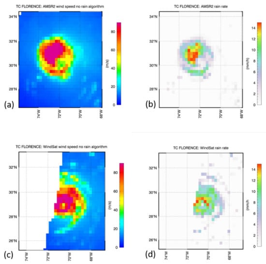
Figure 1.
Passes of AMSR2 and WindSat over Hurricane Florence on 12 September 2018. The AMSR2 overpass occurred at 18:12 UTC. The WindSat overpass occurred at 10:54 UTC. (a) AMSR2 wind speed retrieved from the rain-free algorithm and displayed here even in rainy areas. (b) AMSR2 rain rate. (c) WindSat wind speed retrieved from the rain-free algorithm and displayed here even in rainy areas. (d) WindSat rain rate.
The rain contamination problem can be mitigated for sensors that measure at multiple frequencies in the C-band (4–8 GHz) and X-band (8–12 GHz) range. This is because: (1) at these lower frequencies, atmospheric scattering, whose signature is very difficult to model, is still relatively small, even under heavy rain [15], and the atmospheric attenuation by rain droplets is dominated by Rayleigh absorption. (2) The spectral differences in the brightness temperature (TB) signal that are caused by wind-induced surface emissivity are small between the C- and X-band. On the other hand, the spectral TB differences caused by rain attenuation are larger. It is therefore possible to find combinations between the C- and X-band channels that are practically insensitive to rain attenuation but sensitive to wind-induced surface emission. This allows for the separation of wind signals from rain signals. Using these channel combinations in the wind speed retrieval algorithm makes it possible to reduce wind speed biases associated with precipitation. This basic principle was first employed for the airborne SFMRs (Stepped-Frequency Microwave Radiometers) that are regularly flown onboard hurricane-penetrating aircrafts to measure the wind speed in TCs [16,17,18,19,20,21,22]. The SFMR does this by only utilizing several C-band frequencies. For spaceborne radiometers, all-weather wind speed algorithms have been developed for the WindSat [23,24,25] and AMSR [26,27,28,29,30] sensors, which contain C-band and X-band frequencies.
A crucial part of these all-weather wind speed retrieval algorithms is their training. For rain-free atmospheres, it is generally most effective to develop physical algorithms that are based on a Radiative Transfer Model (RTM) for the top of the atmosphere (TOA) electromagnetic radiation that is emitted by the rough ocean surface and attenuated in the Earth’s atmosphere [1,2,3,4,5]. As pointed out in [23], the difficulty of modeling rain attenuation within an RTM can make algorithms based on simple statistical regressions a better candidate for all-weather wind retrievals. These statistical algorithms are trained from match-ups between TBs that are measured by the sensor under consideration (WindSat, AMSR) and ground-truth wind speed measurements from a reliable external source. The quality of these external ground-truth wind speeds together with the accuracy of the temporal and spatial matching are the main drivers for the quality of the statistical regression algorithm and, consequently, for the accuracy of the all-weather wind speed measurements.
For example, our earlier development of WindSat all-weather wind retrievals was trained using hurricane wind speeds from the H-wind analysis [31,32] that was developed by hurricane researchers and based mainly on input from SFMR and other reliable in situ sources. The availability of the H-winds for match-ups with WindSat TB was quite limited. In particular, high wind events above 35 m/s were sparsely represented and thus the resulting all-weather wind retrievals could be expected to become inaccurate or to break down in strong tropical cyclones.
The goal of this paper is to demonstrate the training of a new all-weather wind algorithm for WindSat, AMSR-E, and AMSR2 with wind speeds from the NASA SMAP (Soil Moisture Active Passive) radiometer [33,34], which operates at L-band (1.41 GHz) [35,36]. L-band radiometers such as SMAP and SMOS (Soil Moisture and Ocean Salinity) have several distinct advantages when it comes to measuring wind speed in strong storms. First, the low frequency implies no or only very minor attenuation by rain [37,38]. Thus, the aforementioned rain contamination problem found at higher frequencies is negligible at L-band. Second, at high wind speeds, the L-band surface emitted TB signal keeps growing approximately linearly with wind speed [33,38,39]. The signal does not lose sensitivity as wind speed increases and does not saturate, even in category 5 tropical storms. This enables L-band radiometers to make reliable wind estimates in strong TCs. This has been demonstrated and tested in several studies that have compared L-band TC wind speeds with various reliable external sources [33,38,39,40,41,42,43].
SMAP and WindSat have approximately the same local ascending node time (about 18:00). This enables us to obtain a large number of WindSat TB–SMAP wind speed match-ups in TCs that can be used in training WindSat all-weather wind speed retrievals, including winds in category 5 storms. This makes SMAP an ideal training set for the WindSat TC-wind algorithm. The local ascending node times of AMSR-E and AMSR2 are at about 13:30. As a TC can change significantly in intensity, size, and shape within 4 ½ h, it is difficult to find good match-ups between AMSR TB and SMAP winds for training an AMSR TC-wind algorithm. However, the channel configurations of frequency and Earth Incidence Angles (EIA) for the WindSat and AMSR instruments are similar. Therefore, it is possible to transfer the TC-wind algorithm that has been trained for WindSat to AMSR after a small TB adjustment that accounts for the frequency and EIA differences between the two sensors.
In this paper, we will mainly focus on the development and testing of wind speed retrievals for WindSat and AMSR, which are trained specifically under TC conditions. These conditions consist of high wind speeds (>15 m/s) and high sea surface temperature (SST > 25°C) as well as potentially high rain rates. We will finally demonstrate how these algorithms can be extended to global all-weather wind-through-rain retrievals and can be run under a wide variety of conditions.
Our paper is organized as follows: Section 2 explains the basic methodology for developing statistical regressions for TC-wind algorithms that utilize WindSat and AMSR C- and X-band channels and that are trained and tested with SMAP wind speeds. We discuss the major error sources in the TC-wind algorithm. We also give a brief account on data production and distribution. In Section 3, we perform a case study that demonstrates the determination of intensity and size of several selected TCs based on these algorithms and how the results fit with external sources that are used by TC forecasters. Section 4 gives an outlook on possibly extending the algorithms from C-X-band to X-K band sensors. Section 5 shows how the algorithms, which have been specifically trained for TC conditions, can be extended to global all-weather wind retrievals. Section 6 summarizes our findings. We want to note that a more detailed and comprehensive assessment of the proposed WindSat and AMSR TC-wind retrievals is presented in a separate article within this Special Issue of Remote Sensing [44].
2. Wind Speed Retrieval Algorithms in Tropical Cyclones for C-X Band Sensors
2.1. TC Match-Up Sets between WindSat Brightness Temperatures and SMAP Wind Speeds
The basis of our new statistical TC-wind algorithm is a match-up set between measured WindSat TBs and measured SMAP wind speeds collected in TCs. The SMAP winds are available as Level 3 global daily maps gridded at 0.25° and separated into ascending and descending swaths [34]. The actual spatial resolution of the SMAP winds is about 40 km.
The WindSat TBs are taken from Level 2 files, in which all WindSat antenna temperature (TA) observations are resampled onto a common fixed 0.25° Earth grid by a Backus–Gilbert type optimum interpolation scheme [45]. The centers of the SMAP wind grid cells coincide with the centers of the d WindSat grid cells. We use the vertically polarized (V-pol) and horizontally polarized (H-pol) C-band (6.9 GHz) and X-band (10.7 GHz) WindSat TA that are both resampled to the C-band spatial resolution, which is about 50 km. These resampled WindSat TAs are then converted into TBs following the calibration procedure outlined in [4,46].
We collect SMAP wind speeds for a series of TCs of category 1 or higher. This means the maximum SMAP wind speed of the TC is at least 33 m/s. The location and times of the TC can be easily identified from meteorological records by the major tropical storm forecast centers, such as the U.S. National Hurricane Center (NHC) or the U.S. Joint Typhoon Warning Center (JTWC). We use data from storms over the 5-year time period from 2015–2019. In each storm, we visually identify the center and then collect wind speeds in all SMAP grid cells whose latitudes and longitudes are within +/− 2°of the storm center. We note that the SMAP sensor is particularly well-suited for these types of high wind speed measurements. However, at lower wind speeds, the sensitivity of the SMAP radiometer observation to wind speed decreases [47], and at the same time, the sensitivity to other environmental parameters, mainly sea surface salinity (SSS), increases. Consequently, the accuracy of the SMAP wind speed measurements decreases at lower winds. Due to this, we only use cells whose SMAP wind speed is at least 13 m/s for our match-up set.
As each SMAP grid cell falls within one WindSat grid cell with the same center and because the ascending node times of SMAP and WindSat fall within a few minutes of each other, it is easy to find records from both sensors whose observation times match within a few minutes. Our approach overlays ascending SMAP swaths with ascending WindSat swaths and descending SMAP swaths with descending WindSat swaths for the same times and chooses the grid cells from the two sensors with the same center. Since the WindSat observations have already been optimally interpolated onto the 0.25° fixed Earth grid and the spatial resolution of the WindSat (≈50 km) and the SMAP observations (≈40 km) are close, additional resampling of the WindSat TBs is not necessary when creating the match-up set.
As the SMAP and WindSat observations in the match-up sets are within a few minutes, we do not have to be concerned about the TC changing in intensity, size, or shape. The match-up set that is constructed this way contains a sufficient number of wind speeds between the lower cut-off 13 m/s up to category 5 storms (70 m/s), and sampling mismatches between SMAP and WindSat are very small. These factors contribute to make SMAP and WindSat the ideal couple for training and testing the TC-wind algorithm. This is a distinct advantage over other all-weather wind algorithms, including our earlier work [23,24].
The WindSat TB–SMAP wind speed set is supplemented with two important ancillary parameters that are used in developing and testing the TC-wind algorithm: SST and surface rain rate. SST is obtained from a monthly climatology, which was derived from the NOAA Optimum Interpolated (OI) SST [48,49]. The SST from the climatology is interpolated in space and time to the WindSat observation. Note, that WindSat SST measurements [10] are not available in precipitation. The surface rain rate R is measured and retrieved directly from WindSat using the higher frequency (18.7, 23.8, 37.0 GHz) channels [10,50,51].
We use half of the match-up set for the years 2015 and 2016 for training of the TC-wind algorithm and reserve the other half of the match-ups for 2015 and 2016 and for all of 2017–2019 for algorithm testing and evaluation.
2.2. C-X Band Combinations with Reduced Rain Contamination
Before describing the details of the TC-wind algorithm for C/X-band sensors, it is instructive to give a brief recap of the basic principle that governs the mitigation of rain contamination.
For the purpose of demonstrating the underlying principle, we assume a simple case of an ocean–atmosphere system at uniform effective temperature Teff. For a non-scattering atmosphere, TOA TB that is emitted by the ocean surface and received by the satellite sensor at the TOA is approximately given by [2,23]:
ρ denotes the reflectivity of the ocean surface and τ denotes the atmospheric transmittance. τ is determined from the atmospheric absorption by water vapor, oxygen and cloud droplets. It thus depends, among other parameters, on the rain rate R.
TB ≈ (1 − ρ·τ2)·Teff
We consider a linear combination of the C-band and X-band TB for a given polarization p =V-pol, H-pol. For typical ocean scenes that are encountered in TCs and for the EIA values of the WindSat and AMSR sensors, the spectral difference in the surface emission is small. Therefore ρ(C-band) ≈ ρ(X-band) ≡ ρ0. Consequently,
TB,C-band − λ ·TB,X-band ≈ − ρ0 ·Teff·[ τC-band 2 − λ·τX-band 2]
The idea is to choose the parameter λ so that the linear combination (2) shows minimal sensitivity to the rain rate R. That means:
∂/∂R [TB,C-band − λ ·TB,X-band] = 0
and thus
and thus
λ ≈ [∂ τC-band 2 /∂R]/[∂ τX-band 2 /∂R
For typical scenes viewed by the WindSat and the AMSR C- and X-band channels, this results in values of λ in the range of 0.3 … 0.4 for both V-pol and H-pol. We can expect that using linear C/X-band channel combinations with values of λ in this range in the TC-wind retrievals will result in reduced sensitivity to rain, and thus, reduced rain contamination.
We note that the surface emissivity, and thus, the surface emitted TB of both the C-band and X-band show very good sensitivity to wind speed at high winds. Similar to L-band, the surface TBs increase approximately linearly with wind speed, and there is no indication that the surface signal will saturate at higher wind speeds [52]. This holds for both V-pol and H-pol. Thus, once the atmospheric attenuation has been removed, radiometers with the C- and X-band channels are very good candidates for measuring wind speeds in strong storms.
Figure 2a and Figure 3 demonstrate this basic principle for a SMAP–WindSat match-up of Hurricane Patricia in the eastern Pacific close to the Mexican coast on 23 October 2015, when it had exceeded category 5 strength. Figure 2a shows the SMAP wind speed, which is regarded the target for the WindSat TC algorithm. A detailed analysis of this particular case, including a comparison between SMAP and SFMR wind speed measurements, was given in [33]. The rain effect is clearly evident when looking at the TB of the individual C-band (Figure 3a) and X-band (Figure 3b) WindSat channels and comparing them with the WindSat rain rate measurement (Figure 3c). For example, the large rain band that is visible in the SE and SW quadrants shows up as artificially high TB in both the C-and X-band channels. As expected, the rain effect is stronger at the X-band than at the C-band. However, in the linear combination TB,C-band − 0.4·TB,X-band (Figure 3d) the rain contamination in that band gets significantly reduced and the resulting TB field resembles the SMAP wind speed field much better than the individual C- and X-band TB do.
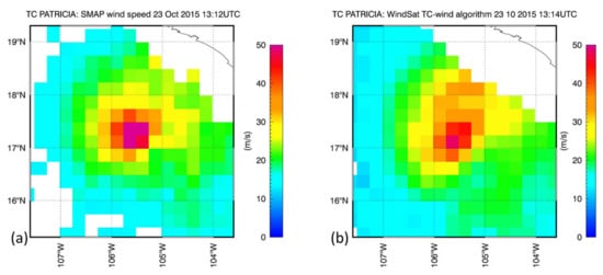
Figure 2.
Passes of AMSR2 and WindSat over Hurricane Patricia on 23 October 2015. (a) SMAP wind speed. The SMAP pass occurred at around 13:12 UTC. (b) WindSat TC-wind speed. The WindSat pass occurred a couple minutes later.
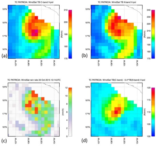
Figure 3.
Basic methodology to minimize rain contamination in TC wind speed retrieval for the WindSat passes over Hurricane Patricia (Figure 2): (a) WindSat 6.8 GHz TB vertical polarization. (b) WindSat 10.7 GHz TB vertical polarization. (c) WindSat rain rate. (d) Combination 6.8 GHz–0.4 ·10.7 GHz V-pol TB. The rain contamination is reduced in this channel combination.
2.3. Statistical Linear Regressions for C/X-Band Channels
The WindSat TC-wind algorithm is a statistical linear regression of the wind speed W against the WindSat TB measurements, which is trained from the SMAP wind speed–WindSat TB match-up set of Section 2.1. The regression has the form:
W = a(R) + ∑i,p bi,p (R)·(TBi,p − T B,off) + ∑i,p ci,p (R)·(TBi,p − TB,off)2
In the sums, the frequency index i runs over C-band and X-band and the polarization index p runs over V-pol and H-pol. We include linear and quadratic terms in TB from both the C- and X-band and both V-pol and H-pol channels. The value of TB,off is set to 150 K. We train a set of algorithms in four different rain intervals based on the value of the WindSat rain rate R as indicated in Table 1. Consequently, the regression coefficients a, bi,p and ci,p in (5) depend on rain rate R. When calculating W from (5) in the retrievals, we linearly interpolate between the values of R listed in the second column of Table 1, which are the population weighted averages in each regime. When the value of R lies outside the range of these interval centers, we do not extrapolate, but rather cut-off the value of R at the lowest and the highest value shown in the second column of Table 1. In choosing the four intervals, we have tried to ensure a sufficient population in each interval. The choice of the rain rate intervals is not unique, and we have checked that the TC-wind retrievals are robust when varying the size of the intervals.

Table 1.
Rain rate intervals used for training the WindSat TC-wind algorithm. The 2nd column contains the population weighted average in each interval.
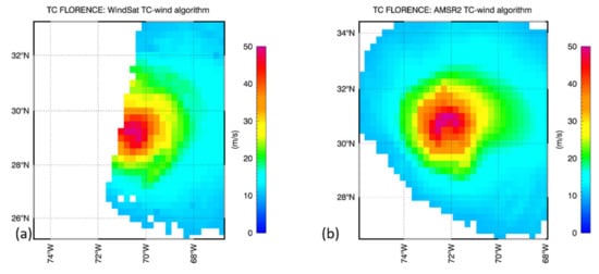
Figure 4 shows scatterplots in three different rain rate regimes of the retrieved WindSat TC-winds versus the SMAP wind speed for winds above 15 m/s when the WindSat TC-wind algorithm is run on the match-up set that was reserved for testing as described in Section 2.1. The statistical results for the bias, standard deviation, and correlation coefficient that are presented in the figure indicate the expected performance of the TC-wind algorithm when compared to SMAP winds. The WindSat TC-wind field of the Patricia overpass case is shown in Figure 2b and closely resembles the result from the linear TB combination (Figure 3d) that we have considered in Section 2.2. We note that in the NE quadrant, where the rain rates are very high, some residual rain contamination in the WindSat TC-wind of Figure 2b is still present. Thus, for very strong precipitation we expect that the TC-wind algorithm performance might degrade but nevertheless constitutes a clear improvement over rain-free algorithms. Figure 5a displays the WindSat TC-wind field for the pass over Hurricane Florence from Section 1. The strong rain contamination that is observed with the standard rain-free algorithm (Figure 1c,d) has been largely reduced. These results demonstrate the capability of the SMAP-trained WindSat C/X- band combination algorithm to retrieve realistic and usable wind speeds in strong TCs.
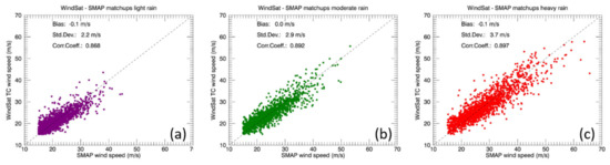
Figure 4.
Testing of WindSat TC algorithm in 3 different rain regimes. The figures show scatterplots between the SMAP and the retrieved WindSat TC wind speeds of the SMAP–WindSat match-up set that was reserved for algorithm testing (Section 2.1). Only observations for which both wind speeds are above 15 m/s are included. (a) Light rain (WindSat rain rate above 0 and below 4 mm/h). (b) Moderate rain (WindSat rain rate above 4 and below 8 mm/h). (c) Heavy rain (WindSat rain rate above 8 mm/h). The values of the bias, standard deviation and the linear correlation coefficient are indicated in each plot.
2.4. AMSR TC-Wind Algorithm
The TC-wind algorithm for the AMSR-E and the AMSR2 sensors requires an additional step due to the fact that the ascending node times of the AMSR and SMAP radiometers differ by about 4 ½ hours. During that time period, a TC can undergo significant changes in intensity, size, and shape. Therefore, constructing a match-up set with SMAP winds, as we did for training the WindSat algorithm, is difficult as it would result in a significant sampling mismatch. Moreover, the center frequencies and EIA of the AMSR and WindSat differ (Table 2) and thus the TOA TBs also differ. Therefore, the statistical regressions (5) that were derived for WindSat in Section 2.3 cannot be directly applied to the AMSR TBs.
Table 2.
Values of the center frequencies and nominal Earth Incidence Angles (EIA) for the WindSat and AMSR C-band and X-band channels.
Similar to WindSat, the AMSR C- and X-band TA measurements are optimally interpolated to a common location and to the spatial resolution of the C-band (≈50 km) and subsequently converted into TBs. For AMSR, the resampling and calibration procedure is outlined in [53,54,55]. There is a subtle difference between the optimum interpolation schemes WindSat and AMSR. For AMSR, the sampling is carried out on a swath grid, which is based on the actual AMSR scanning geometry, rather than on the fixed Earth grid that was employed for WindSat. Scanning and swath geometry for AMSR are simpler than for WindSat and thus it is possible to process AMSR retrievals directly on the swath grid. For the TC-wind algorithm, the grid and resampling differences have no major impact.
In order to transfer the WindSat TC-wind algorithm to AMSR, we first need to adjust the AMSR C- and X-band TB measurements from the AMSR to the values of the WindSat frequency f and EIA θ. This adjustment can be performed using the same RTM that is used for computing the TOA TB [2,52,56,57] and then applying the shift:
(TB, AMSR)adj = (TB, AMSR)measured + [TB,RTM (fWindSat, θWindSat) − TB,RTM (fAMSR, θAMSR)]
This technique is frequently referred to as the double difference method. The shift is performed for each channel separately using the values for f and θ from Table 2. The statistical regression algorithm for WindSat (5) can then be run on the adjusted AMSR TB.
The RTM computation in (6) requires several geophysical input parameters. For the atmospheric part, we use the bulk formulas from [2]. The sea-surface temperature TS is again taken from the monthly climatology based on the NOAA OI SST [49]. The values for columnar water vapor V, columnar cloud liquid water L, and the rain rate R, are retrieved from AMSR using the higher frequency channels at 18.7, 23.8, 36.5 GHz [8,9]. For the value of wind speed, which contributes to the surface emissivity, we use a value of 15 m/s, which is typical for the conditions we encounter in TC. We note that the RTM computation in (6) only needs to calculate the TB differences between the WindSat and AMSR configurations given in Table 2. These differences are small. Therefore, the TB difference computation is much more robust against any uncertainties in the RTM or the geophysical input than the RTM computations of the TB themselves. When taking the difference, these uncertainties cancel to a large degree.
We use the same TC-wind algorithm for AMSR-E and AMSR2, which utilizes the 6.925 GHz (C-band) and 10.65 GHz (X-band) channels. AMSR2 has additional C-band channels at 7.3 GHz V-pol and H-pol that we do not use, as they do not have counterparts in WindSat and thus the corresponding TB adjustment (6) would be less accurate. We note that there are other approaches for developing AMSR2 winds in storms that do utilize these 7.3 GHz channels [27,28,29].
Figure 5b shows the AMSR2 TC-wind field for Hurricane Florence and is to be compared with the unrealistic result from the rain-free algorithm from Figure 1a. Figure 6 shows the AMSR-E TC-wind for the well-known example of Hurricane Katrina. In both instances, the AMSR TC-winds are very realistic in size and intensity. We will elaborate on this further and conduct a comparison with external sources in Section 3.
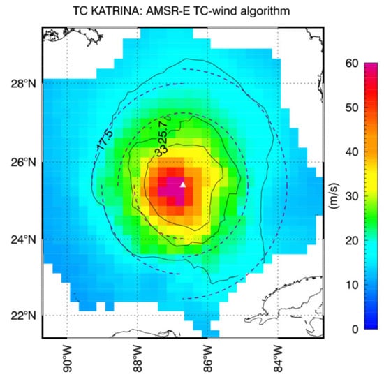
Figure 6.
TC wind speed retrievals of the AMSR-E passes over Hurricane KATRINA on 2005/08/28 07:32 UTC. The full lines are the TC-wind contours of the 17.5 m/s (34 kt, gale-force), 25.7 m/s (50 kt, storm force) and 33 m/s (64 kt, hurricane force) winds. The dashed lines indicate the gale-force and storm force radii in the 4 quadrants (NE, SE, SW, NW) from the Best-Track (BT) data provided by the US National Hurricane Center (see the discussion in Section 3).
2.5. Error Sources
We now list and briefly discuss the major error sources that enter the TC-wind retrieval algorithm:
- There is radiometer noise, calibration uncertainties or pointing errors in the WindSat or AMSR TB. These uncertainties already enter into standard rain-free wind speed retrievals. From validation studies that have been performed [1,6,7], we can estimate their magnitude amount to wind speed errors of 1 m/s or less.
- Wind direction error: We have neglected wind direction in the TC-wind retrievals. The size of the wind direction signal in the surface emissivity at the C- and X-band ranges from about 1 K at 15 m/s to 2 K at very high winds [52], which translates into an error of at least 1–2 m/s in the retrieved wind speeds.
- There might be environmental parameters other than wind speed or direction that could impact the ocean surface roughness and the microwave emission from it (e.g., wave height or wave direction).
- There are uncertainties in the radiometer rain rate R that is used as input to the regression (5).
- For the AMSR TC-wind retrieval, there can be errors in the RTM adjustment (6) or in the input parameters that are needed in the computation of (6), such as SST, V, L and R.
- There is variability in the atmospheric conditions that are present within the TC, in particular the atmospheric moisture and temperature.
- In very heavy precipitation (10 mm/h rain rate and higher), the contribution of atmospheric scattering by rain droplets starts increasing for the higher X-band frequency channels. We have neglected scattering in our approach. The argument from Section 2.2. breaks down and so does the training of the TC-wind algorithm from Section 2.3. Atmospheric scattering leads to a decrease in the TOA TB and thus has the opposite effect from atmospheric absorption, which increases the TOA TB [15]. Therefore, atmospheric scattering can result in a negative bias in the retrieved wind speed.
- There is noise in the SMAP wind speeds that were used for training the WindSat TC-wind algorithm.
With the exception of the first two items, it is difficult to give a quantitative estimate for the single sources in this list. An estimate of the total retrieval uncertainty and an estimate of the algorithm performance can be made from the standard deviation values for the algorithm testing that are given in Figure 4.
2.6. Data Processing and Distribution
Remote Sensing Systems (RSS) processes and distributes daily global TC-wind maps in netCDF4 format for SMAP, WindSat, AMSR-E and AMSR2 (http://www.remss.com/tropical-cyclones/tc-winds/). For SMAP and AMSR2, which are currently operating, the processing is carried out in near-real time (NRT) with a latency of about 2 h, and the daily maps are updated as soon as a new orbit has been processed. The maps are gridded at 0.25° and separated into ascending and descending swaths. In addition to the TC-wind speed, each grid cell also contains the time of observation. The WindSat maps also contain the values for wind direction, rain rate, and ancillary SST. The AMSR-E and AMSR2 maps also contain the values for rain rate, columnar water vapor, and ancillary SST.
The TC-wind algorithms for WindSat and AMSR have been trained specifically under TC conditions, which comprise high wind speeds and high SST. One should expect that the algorithm breaks down if these conditions are not met. For this reason, the daily TC-wind maps contain no data if the ancillary SST is below 20°C or the retrieved wind speed is below 10 m/s.
3. Time Series of Intensity and Size of Selected Tropical Cyclones
The TC-wind retrievals from AMSR, WindSat, and SMAP allow for an easy determination of parameters that are used by TC forecasters and warning centers to characterize the size, shape, and strength of the storms [58,59,60,61,62,63,64,65,66,67,68,69]. These are:
- The storm intensity, which is defined as the maximum 1-min sustained wind speed.
- The maximum radii of the gale-force (34 kt, 17.5 m/s), storm-force (50 kt, 25.7 m/s) and the hurricane force (64 kt, 33 m/s) winds, labelled R34, R50, R64, in each quadrant NE, SE, SW, NW.
Another important storm parameter is the radius of maximum wind speed, which characterizes the distance from the storm center to the eyewall of the cyclone. However, the spatial resolution of the satellite winds that we consider (40–50 km) is in most instances not sufficient to determine this parameter and therefore, we will not consider it here.
In this section, we will compute and compare intensity and radii from the two AMSR, WindSat, and SMAP with estimates from the Best Track (BT) data [59,61] for several selected storms. These BT data are collected and distributed by the U.S. National Hurricane Center (NHC) [70] for TC in the Atlantic and eastern Pacific basins and by the U.S. Joint Typhoon Warning Center (JTWC) [71] for the other four basins (Central Pacific, western Pacific, Southern Hemisphere, and Indian Ocean). They are based on a consensus on data sources and methods that the forecasters are confident in. In the few instances where SFMR measurements from hurricane-penetrating aircrafts are available, those are used in the BT data. If no SFMR observations exist, estimates for the BT R34 radii are mostly based on measurements from the European Advanced Scatterometer ASCAT [72], which are considered a reliable source. There is much less confidence in the values of the R50 radii and even less in the R64 radii. We will not consider R64 for our comparisons. The BT estimates for the TC intensity largely rely on the Dvorak technique [58,60] or refinements of it [73]. These methods are based on cloud pattern recognition from visible and infrared satellite sensors. One needs to be aware that this is an indirect technique for determining the maximum wind speed in a TC, and there are uncertainties associated with it [62]. In addition to the BT data, the SATCON archive [74,75] of the Cooperative Institute for Meteorological Satellite Studies at the University of Madison-Wisconsin is a very valuable database for intensity estimates of TCs that we have used for our comparisons. It is based on a consensus approach using numerous data sources and also provides an estimate of the uncertainties that are associated with the recorded intensity values.
Before presenting the results of the comparison, we need to mention and discuss the difference in spatial and temporal scales that come into play when estimating TC intensities. The BT and SATCON intensity values refer to 1-min sustained maximum winds and the sources of the estimate are generally of high spatial resolution, on the order of a few km or better. The spatial resolution of the satellite sensors in our study is significantly coarser (40–50 km). Consequently, our satellite maximum winds are lower that then BT or SATCON estimates as the satellite measures an average over a larger spatial scale. In general, the relation of TC intensity estimates from observations at different spatial scales depends on the size, structure, and strength of the TC wind field itself [76]. As a rule of thumb, the TC intensity estimates from the AMSR, WindSat, and SMAP satellites should be considered as corresponding to a 10-minute sustained wind. Therefore, in order to allow a better comparison of our results with the BT and SATCON values, we have scaled the BT and SATCON intensities from 1-minute to 10-minute sustained winds using a factor of 0.93 that has been recommended by the WMO [77]. A detailed methodology of comparing TC-wind fields from our AMSR, WindSat, and SMAP algorithms with wind fields for the high spatial resolution HWRF (Hurricane Weather Research and Forecasting) model is presented in [44].
When computing the radii of our satellite TC-winds, we first visually identify the storm center. Although the values of the storm radii are formally defined as the maximum radius for each of the wind contours in each quadrant, we report the upper value of the 80 percentile. This is carried out because there is considerable noise in the retrieved satellite winds, which can result in outliers if the actual maximum radius is reported. An example for the wind radii determination from the AMSR-E TC-wind compared to BT is shown in Figure 6 for the case of Katrina.
The following cases were selected to allow a comparison between our satellite TC-winds and BT or SATCON data for the time series of numerous passes over the same storm, and thus, an assessment of the time evolution of the size and strength of the cyclone over the lifetime of the storm. Of particular interest are cases with large changes of the storm intensity that occur within a short time period, known as rapid intensification [78]. We only show cases where the extent of the satellite view is sufficient to determine intensity and radii.
Figure 7 shows the intensity time series for Hurricane Katrina, as seen by WindSat and AMSR-E compared to BT.
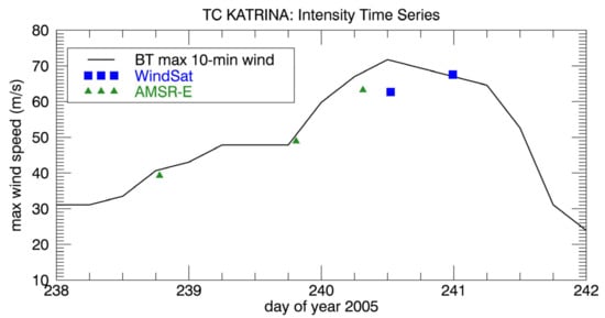
Figure 7.
Intensity (maximum wind speed) time series of TC winds from AMSR-E (green triangles) and WindSat (blue squares) passes over Hurricane Katrina in 2005. The black line indicates the intensity time series of the BT data after scaling them to 10-min sustained winds to better match the scales seen by the satellite sensors.
The intensity time series from AMSR2, WindSat, and SMAP are displayed in Figure 8 for Hurricane Florence and in Figure 9 for Super Typhoon Mangkhut, compared to SATCON. The Mangkhut radii time series compared to BT are shown in Figure 10 for R34 SE and in Figure 11 for R50 SE.
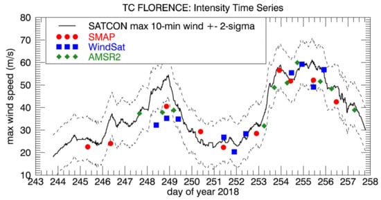
Figure 8.
Intensity (maximum wind speed) time series of TC winds from SMAP (red circles), AMSR2 (green diamonds) and WindSat (blue squares) passes over TC Florence in 2018. The solid black line indicates the intensity time series of the University of Wisconsin SATCON data after scaling them to 10-min sustained winds. The dashed black lines indicate the +/−2-sigma deviation of the SATCON data.
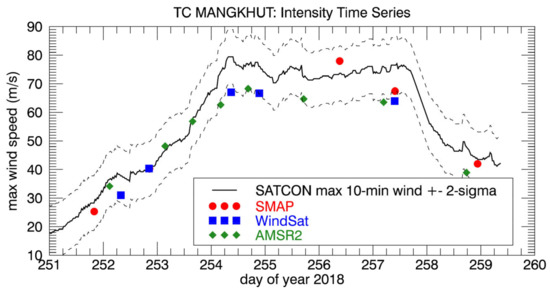
Figure 9.
Intensity (maximum wind speed) time series of TC winds from SMAP (red circles), AMSR2 (green diamonds) and WindSat (blue squares) passes over Super Typhoon Mangkhut in 2018. The solid black line indicates the intensity time series of the University of Wisconsin SATCON data after scaling them to 10-min sustained winds. The dashed black lines indicate the +/−2-sigma deviation of the SATCON data.
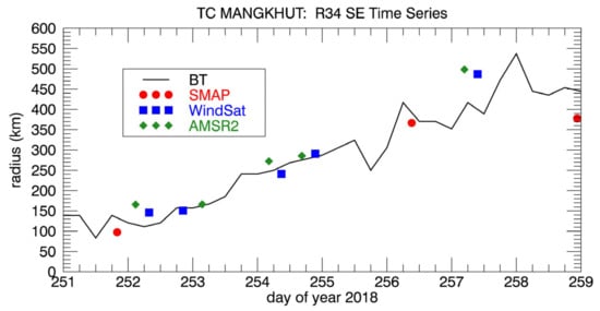
Figure 10.
Time series of R34 (34 kt, 17.5 m/s, gale-force winds) in the SE sector from SMAP (red circles), AMSR2 (green diamonds) and WindSat (blue squares) passes over Super Typhoon Mangkhut in 2018. The black line indicates the R34 radii time series of the BT data.
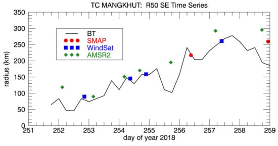
Figure 11.
Time series of R50 (50 kt, 25.7 m/s, storm-force winds) in the SE sector from SMAP (red circles), AMSR2 (green diamonds) and WindSat (blue squares) passes over Super Typhoon Mangkhut in 2018. The black line indicates the R50 radii time series of the BT data.
In general, we observe good agreement between the satellite-derived parameters and the BT and SATCON values. The satellite TC-winds are more than capable of tracking the evolution of the strength and size of the storms over the lifetime of the TC. We also note consistency among the three satellites SMAP, AMSR, and WindSat. This is, of course, largely due to the fact that both AMSR and WindSat TC-wind algorithms have been trained from SMAP winds.
In order to aid the routine ingestion of the TC-winds into the Automated Tropical Cyclone System (ATCF) by the U.S. Navy and the JTWC, we have augmented the NRT TC-wind fields (Section 2.6) with simple text files in ATCF [59] format that contain values of the storm intensity and radii. The automated NRT determination of the storm radii requires knowledge of the storm center. Our current processing obtains the storm center coordinates from TC track forecasts. In the future, we will consider using an automatic storm center determination based on the MTrack method that has been developed by [79].
4. Extension to X-K Band Sensors
The number of present and planned passive microwave sensors that operate at the C-band is very limited. It is therefore desirable to be able to apply a similar technique as we have developed for the WindSat and AMSR TC-winds to instruments that operate at higher frequencies. Absorption and scattering by rain both increase with increasing frequency. In order to keep the degradation due to rain contamination as small as possible in the absence of C-band, the best option is a TC-wind algorithm that uses X-band and Ku- or K-band frequencies.
We have performed a preliminary study for a TC-wind algorithm using the WindSat 10.7 and 18.7 GHz channels and present some first results in this section. The training and basic testing of this algorithm follows the same steps of the WindSat C/X-band algorithm that was laid out in Section 2.3. In the regression (5), the 6.8 GHz V-pol and H-pol TB are swapped for the 18.7 GHz V-pol and H-pol TB and new regression coefficients are derived from the WindSat 10.7/18.7 TB–SMAP wind speed match-up set.
Figure 12 shows the scatterplot between WindSat TC-winds and the SMAP winds, which can be directly compared to the corresponding results of the WindSat C/X-band algorithm from Figure 4. The statistics for the case of light rain (rain rate larger than 0 and up to 4 mm/h, Figure 4a and Figure 12a) are very close in both algorithms. This indicates that training a X/K-band TC-wind algorithm is feasible in light rain. At higher rain rates, the degradation of the X/K-band compared to the C/X-bands results is noticeably stronger. This is not surprising, as we expect that atmospheric scattering by rain becomes stronger in high precipitation for the K-band channels. As noted in Section 2.5., this can lead to a decrease in the K-band TB in high rain, which will result in a decrease of the retrieved wind speeds. The scatterplots in Figure 12b,c indicate that this is indeed the case.
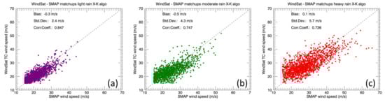
Figure 12.
Same as in Figure 4 but using the WindSat X-K-band TC-wind algorithm.
Figure 13 shows the TC-wind fields of Typhoon Haima as seen by SMAP (Figure 13a), WindSat C/X-band (Figure 13c), and WindSat X/K-band (Figure 13d). The WindSat rain rate is also shown (Figure 13b). The rain contamination in the outer rain band, in particular in the SW and SE sectors, is evident in the X/K-band winds when compared to the C/X-band winds. Nevertheless, the size, shape, and intensity of the cyclone that is measured by the X/K-band algorithm compares well with the C-X-band winds and also to the SMAP winds. Despite the increased rain contamination, it might still be possible to extract usable measurements of the storm intensity and radii. We will perform further studies to explore the extent to which this can be carried out. A possible extension of the TC-wind algorithm to X/K-band would make it possible to include several additional sensors, such as the Tropical Rainfall Measurement Mission Microwave Imager (TMI) [80], the Global Precipitation Mission Microwave Imager (GMI) [81], and also the Weather System Follow-on Mission Microwave Imager (WSF-MWI) [82,83], whose launch is planned for 2023.
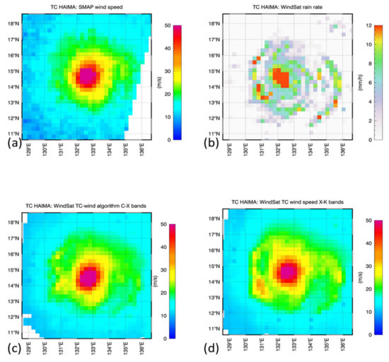
Figure 13.
SMAP and WindSat passes over Typhoon Haima on 10/17/2016. Both overpasses occurred within 5 min at around 21:25 UTC. (a) SMAP wind speed. (b) WindSat rain rate. (c) WindSat TC-wind speed using the C-X-band algorithm. (d) WindSat TC-wind speed using the X-K-band algorithm.
5. Extension to Global All-Weather Wind Retrievals
The AMSR and WindSat TC-wind algorithms were trained specifically for TC conditions, which comprise high SST and high winds. We expect that the algorithm performance quickly degrades when applied to cases that do not meet the conditions of the training set. In order to retrieve winds through rain globally, including ETCs or in areas with tropical convection, it is necessary to take additional steps. This is described in this section.
5.1. WindSat—SMAP—NCEP Match-Up Set
Using SMAP wind speeds to train winds-through-rain algorithms is appropriate at high wind speeds (>15 m/s), where the SMAP winds are reliable. However, at lower wind speeds, the SMAP winds become less accurate. There are several reasons for this. First, the L-band wind-induced emissivity signal loses sensitivity to wind speed in both polarizations between 5–10 m/s. Second, the SMAP wind speed algorithm requires SSS as an external input, which is obtained from a salinity climatology. During heavy rain events and at lower wind speeds, significant SSS stratification occurs in the upper ocean layer [84], which results in less accurate external SSS input from climatology and therefore less accurate L-band wind speeds.
In order to train the global C/X-band all-weather algorithm, we have created a match-up set of triple collocations containing WindSat TB and wind speeds from SMAP and the NCEP Global Data Assimilation System (GDAS) model [85]. The NCEP winds come gridded at 0.25° and every 6 h. We have linearly interpolated the NCEP scalar wind speeds in space and time to the WindSat TB observation. The allowed time difference between SMAP and WindSat TB is at most 30 min.
In general, the confidence in SMAP is good at higher wind speeds but not as good at lower wind speeds. Conversely, the confidence in NCEP is good at lower wind speeds but not as good at higher wind speeds. We have observed very good match-up between SMAP and NCEP winds between 15 and 20 m/s. For training and testing the global all-weather winds algorithm, we first check the NCEP wind speed and use it if it is less than 20 m/s. Next, we check the SMAP wind speed and use it if it is above 15 m/s. If the SMAP wind speed is less than 15 m/s and the NCEP wind speed is above 20 m/s, we discard the observation. Note that this happens very rarely.
The match-up set comprises all the WindSat–SMAP TC match-ups from Section 2.1. In addition, we include orbits containing observations from all seasons and several orbits that include strong ETC. The total size of the match-up set is 409 WindSat orbits. As we did for the TC match-up set, we augment each match-up with the WindSat rain rate and the ancillary NOAA OI SST. We reserve all observations from the ascending WindSat swath for algorithm training and all observations from the descending WindSat swaths for algorithm testing.
5.2. Training of the Global All-Weather Wind Algorithm
The global all-weather retrieval is performed in a two-stage regression. In the training of each stage, it is necessary to include SST as additional parameter. Both ocean surface emissivity and the absorption by cloud liquid water depend on surface temperature. Therefore, the global algorithm needs to be trained differently in different SST regimes. The regression coefficients (5) of the global all-weather algorithm depend both on rain R and on SST TS. The training of this first stage regression is carried out in several rain rate intervals and in several TS intervals, as indicated in Table 3. The size of the intervals is chosen to ensure the sufficient population of each bin when performing the training. In order to achieve sufficient bin population, we let the adjacent R and TS intervals overlap. We keep track of the population weighted averages in each R bin and each TS bin. In the retrieval, we linearly interpolate between the interval center values for R and TS. If the ancillary input values fall outside the interval centers, we do not extrapolate but cut them off at the low or high ends. This completes the first stage regression for the global all-weather winds.
Table 3.
Intervals of rain Rate R, SST TS, and wind speed W that are used in the training of the 1st and 2nd stages of the global all-weather wind speed algorithms. The intervals overlap and are chosen to ensure sufficient population in each bin.
Due to the large wind speed range in the global algorithm, it is beneficial to add a second stage regression that refines the retrieval. The method was developed and laid out in [3] for standard rain-free wind speed retrievals. In the second stage, the regressions are trained in different wind speed intervals, and thus, the regression coefficients in (5) now depend on three parameters: R, TS, and wind speed W. The value of W is obtained from the first stage regression both in the algorithm training as well as when running the retrievals. Overlapping R, TS, and W intervals are used in the algorithm training (Table 3). Note that different R intervals were chosen for the first and second stage. The reason for the interval choice is, again, to ensure a sufficient population in each interval when training the algorithm. In the retrievals, we tri-linearly interpolate between each (R, TS, W) interval center. In the second stage regression, we only include terms that are linear in TB and omit the quadratic terms in (5). In each of the wind speed intervals (Table 3), the relationship between TB and W is approximately linear and adding higher order terms might result in over-fitting. This completes the second stage regression for the global all-weather winds.
When applying the global all-weather wind retrieval to AMSR, we adjust the measured AMSR TB to the WindSat frequency and EIA configuration using the RTM difference (6), as explained in Section 2.4.
Figure 14 shows the two-dimensional pdf between global all-weather AMSR2 and NCEP wind speed for all AMSR2 observations in rain during the whole year of 2019 in three rain regimes. The standard deviations of the wind speed differences AMSR2–NCEP are 1.99 m/s in light rain, 3.03 m/s in moderate rain and 3.67 m/s in heavy rain. For reference, the AMSR2-NCEP standard deviation using rain-free AMSR2 retrievals is approximately 1.2 m/s.
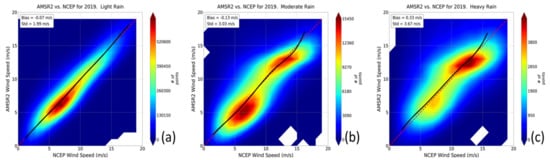
Figure 14.
2-dimensional probability density function between global AMSR2 all-weather wind speeds (y-axis) and NCEP wind speeds (x-axis), for different rain regimes. The dashed red line indicates the 1:1 (y = x) line. The full black line indicates the symmetrized binned averages, which are obtained by binning y with respect x, x with respect to y, and taking the arithmetic average between the two cases. The bin sizes are 1 m/s. (a) Light rain (AMSR2 rain rate above 0 and below 4 mm/h). (b) Moderate rain (AMSR2 rain rate above 4 and below 8 mm/h). (c) Heavy rain (AMSR2 rain rate above 8 mm/h). The values of bias and standard deviation are also indicated in each plot.
5.3. Validation with Buoy Wind Speeds
It is desirable to validate the global all-weather wind speed retrievals with an independent in situ source, such as buoys. We have collected match-ups between AMSR2 all-weather winds and buoy observations from three sources: (1) the National Data Buoy Center (NDBC) [86,87], which includes the tropical TAO buoy array [88]; (2) The Pacific Marine Environmental Laboratory (PMEL) [89], which includes buoys from the PIRATA [90] and RAMA [91] arrays; (3) the Canadian Marine Environmental Data Section (MEDS) [92,93]. For a valid match-up, we require that the AMSR2 wind measurements falls within +/−30 min of an hourly averaged buoy observation and that the center of the 0.25° AMSR2 grid cells is within 25 km of the buoy location. Satellite wind measurements correspond to 10-m neutral stability winds. Therefore, all buoy measurements were converted to 10-m neutral stability winds in order to allow comparison to the satellite winds. Details on comparing buoy and satellite wind measurements can be found in [94]. The AMSR2–Buoy match-up set comprises 3 years of data 2017–2019.
Figure 15 displays the AMSR2–buoy statistics. The results are consistent with the AMSR2–NCEP statistics from Figure 14. For comparison, the AMSR2–buoy standard deviation of the standard no-rain algorithm run in rain-free scenes is 0.96 m/s. When plotted as a function of rain rate (Figure 15b) the standard deviation of the AMSR2 all-weather algorithm increases gradually up to rain rates of about 10 mm/h. For rain rates above 12 mm/h, the errors in the all-weather winds are large enough that the data become unusable for most practical applications.
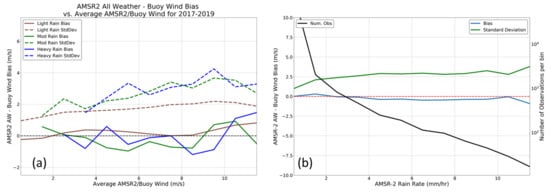
Figure 15.
Comparison between global AMSR2 all-weather and buoy wind speeds. (a) Bias (full lines) and standard deviation (dashed lines) of the AMSR2–buoy wind speed difference as function of the average between AMSR2 and buoy wind speed. The 3 colors indicate 3 different rain regimes: Brown = light rain (AMSR2 rain rate above 0 and below 4 mm/h). Green = moderate rain (AMSR2 rain rate between 4 and 8 mm/h). Blue = heavy rain (AMSR2 rain rate above 8 mm/h). (b) Bias (blue) and standard deviation (green) of AMSR2–buoy wind speed as function of AMSR2 rain rate using 1 mm/h bins. Observations in which the buoy wind speed exceeds 15 m/s have been excluded. The black line indicates the number of observations in each rain rate bin.
5.4. Example of Extra-Tropical Cyclone
Finally, Figure 16 shows an example of a strong ETC in the northern Pacific. There are good views of the storm, as seen by AMSR2, WindSat, and the ASCAT-B scatterometer [95] within 8 h on the same day. The sizes, shapes, and strength of the wind fields from the three satellites compare very well. In general, ETCs do not change as rapidly in size and intensity as it is often the case for TCs. Thus, the comparison of satellite passes that are several hours apart is meaningful for ETCs. We note that there is no strong rain contamination visible in any of the three satellite wind fields.
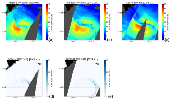
Figure 16.
Example of all-weather wind speeds from AMSR2 and WindSat in a strong extra-tropical cyclone, which occurred on 12/24/2018 in the northern Pacific. (a) AMSR2 all-weather wind. (b) WindSat all-weather wind. (c) For comparison we show the wind from the ASCAT-B scatterometer processed by the RSS algorithm [95]. (d) AMSR2 rain rate. (e) WindSat rain rate.
6. Summary and Conclusions
Ocean wind speed retrieval algorithms for passive microwave sensors that are trained in non-precipitating atmospheres perform well if there is no rain but quickly degrade and break down in precipitation. Radiometers that operate at C-band and X-band frequencies, such as WindSat and AMSR, allow for the training of statistical winds-in-rain algorithms. It is possible to combine the different frequencies so that the effects of rain absorption are reduced, but the sensitivity to surface wind speed is maintained.
We have shown how to train wind speed retrieval algorithms in tropical cyclone conditions from match-up sets between WindSat TB measurements and wind speeds from the L-band radiometer SMAP. The SMAP sensor provides reliable high wind speed observations that are not or are minimally affected by precipitation. The orbital configuration of the SMAP and WindSat sensors is such that both sensors observe the same Earth location very close in time, which is ideal for training a statistical regression algorithm. The WindSat all-weather wind algorithm can be transferred to the AMSR configuration by making a small adjustment to the AMSR TB measurements using a radiative transfer model in order to account for small differences in viewing geometry and frequency.
We have presented case studies that demonstrate the usefulness of the WindSat and AMSR TC-winds for determining size, shape, and strength of tropical cyclones up to category 5. Radii and intensity estimate from our SMAP, WindSat, and AMSR2 TC-wind field retrievals are currently being routinely ingested by several tropical storm warning centers.
We have shown how the algorithms can be extended from tropical cyclone conditions to global all-weather wind retrievals and run in ETCs and areas of tropical convection.
A preliminary study using X-band and K-band frequencies indicates limited potential to train winds through rain algorithms also for X/K -band sensors.
Author Contributions
Conceptualization, T.M.; methodology, T.M., L.R. and A.M..; software, T.M.; formal analysis, T.M. and A.M.; investigation, T.M., L.R. and A.M.; resources, T..M., L.R. and A.M.; data curation, T.M., L.R. and A.M.; writing—original draft preparation, T..M.; writing—review and editing, T.M., L.R. and A.M.; visualization, T.M., L.R. and A.M.; supervision, T..M. and L.R.; project administration, T.M.; funding acquisition, T.M. and L.R. All authors have read and agreed to the published version of the manuscript.
Funding
This research was funded under NASA contacts NNH17CA04C (SMAP Science Utilization), 80HQTR19C0003 (Ocean Vector Winds Science Team), NNH15CN50C (Earth Science U.S. Participating Investigator) and 80HQTR18C0035 (The Science of Terra Aqua Suomi NPP).
Data Availability Statement
The Remote Sensing Tropical Cyclone wind speeds for SMAP, AMSR-E, AMSR2 and WindSat are publicly available at http://www.remss.com/tropical-cyclones/tc-winds/ (accessed on 30 March 2021).
Acknowledgments
We would like to thank John Knaff (NOAA/Center for Satellite Applications and Research, Fort Collins, CO, USA) and Charles Sampson (Naval Research Laboratory, Monterey, CA, USA) for numerous useful discussions and comments.
Conflicts of Interest
The authors declare no conflict of interest. The funders had no role in the design of the study; in the collection, analyses, or interpretation of data; in the writing of the manuscript, or in the decision to publish the results.
References
- Wentz, F. A well-calibrated ocean algorithm for special sensor microwave/imager. J. Geophys. Res. 1997, 102, 8703–8718. [Google Scholar] [CrossRef]
- Wentz, F.; Meissner, T. Algorithm Theoretical Basis Document (ATBD), Version 2, AMSR Ocean Algorithm, RSS Tech. Report 121599A-1, Remote Sensing Systems, Santa Rosa, CA, 66 p. 2000. Available online: http://images.remss.com/papers/rsstech/2000_121599A-1_Wentz_AMSR_Ocean_Algorithm_ATBD_Version2.pdf (accessed on 14 February 2021).
- Wentz, F.; Meissner, T. Algorithm Theoretical Basis Document (ATBD), Supplement 1, AMSR Ocean Algorithm, RSS Tech. Report 1051707, Remote Sensing Systems, Santa Rosa, CA, 6 pp. 2006. Available online: http://images.remss.com/papers/rsstech/2007_051707_Wentz_AMSR_Ocean_Algorithm_Version_2_Supplement1_ATBD.pdf (accessed on 14 February 2021).
- Meissner, T.; Wentz, F. Ocean Retrievals for WindSat. In Proceedings of the IEEE MicroRad, San Juan, PR, USA, 28 February–8 March 2006; pp. 119–124. Available online: http://images.remss.com/papers/rssconf/Meissner_microrad_2006_puertorico_windsat.pdf (accessed on 14 February 2021). [CrossRef]
- Bettenhausen, M.; Smith, C.; Bevilacqua, R.; Wang, N.-Y.; Gaiser, P.; Cox, S. A nonlinear optimization algorithm for WindSat wind vector retrievals. IEEE Trans. Geosci. Remote Sens. 2006, 44, 597–610. [Google Scholar] [CrossRef]
- Wentz, F. A 17-Yr Climate Record of Environmental Parameters Derived from the Tropical Rainfall Measuring Mission (TRMM) Microwave Imager. J. Clim. 2015, 28, 6882–6902. [Google Scholar] [CrossRef]
- Wentz, F.; Ricciardulli, L.; Rodriguez, E.; Stiles, B.W.; Bourassa, M.A.; Long, D.; Hoffman, R.N.; Stoffelen, A.; Verhoef, A.; ONeill, L.W.; et al. Evaluating and extending the ocean winds data climate record. J. Select. Topics Appl. Earth Observ. Remote Sens. 2017, 99, 2165–2185. [Google Scholar] [CrossRef]
- Wentz, F.; Meissner, T.; Gentemann, C.; Brewer, M. Remote Sensing Systems AQUA AMSR-E Daily Environmental Suite on 0.25 deg grid, Version 7.0, Wind Speed, Water Vapor, Cloud Liquid Water and Rain Rate. Remote Sensing Systems, Santa Rosa, CA. 2014. Available online: www.remss.com/missions/amsr (accessed on 14 February 2021).
- Wentz, F.; Meissner, T.; Gentemann, C.; Hilburn, K.; Scott, J. Remote Sensing Systems GCOM-W1 AMSR2 Daily Environmental Suite on 0.25 deg grid, Version 8.0, Wind Speed, Water Vapor, Cloud Liquid Water and Rain Rate. Remote Sensing Systems, Santa Rosa, CA. 2014. Available online: www.remss.com/missions/amsr (accessed on 14 February 2021).
- Wentz, F.; Ricciardulli, L.; Gentemann, C.; Meissner, T.; Hilburn, K.; Scott, J. Remote Sensing Systems Coriolis WindSat Daily Environmental Suite on 0.25 deg grid, Version 7.0.1, Wind Speed and Rain Rate. Remote Sensing Systems, Santa Rosa, CA. 2013. Available online: www.remss.com/missions/windsat (accessed on 14 February 2021).
- Kawanishi, T.; Sezai, T.; Ito, Y.; Imaoka, K.; Takeshima, T.; Ishido, Y.; Shibata, A.; Miura, M.; Inahata, H.; Spencer, R.W. The Advanced Microwave Scanning Radiometer for the Earth Observing System (AMSR-E), NASDA’s contribution to the EOS for global energy and water cycle studies. IEEE Trans. Geosci. Remote Sens. 2003, 41, 184–904. [Google Scholar] [CrossRef]
- Imaoka, K.; Kachi, M.; Kasahara, M.; Ito, N.; Nakagawa, K.; Oki, T. Instrument performance and calibration of AMSR-E and AMSR2. In International Archives of the Photogrammetry, Remote Sensing and Spatial Information Science; International Society for Photogrammetry and Remote Sensing: Kyoto, Japan, 2010; Volume 38, pp. 13–16. Available online: https://www.isprs.org/proceedings/XXXVIII/part8/pdf/JTS13_20100322190615.pdf (accessed on 14 February 2021).
- Oki, T.; Imaoka, K.; Kachi, M. AMSR instruments on GCOM-W1/2: Concepts and applications. In Proceedings of the 2010 IEEE International Geoscience and Remote Sensing Symposium, Honolulu, HI, USA, 25–30 July 2010; pp. 1363–1366. [Google Scholar] [CrossRef]
- Gaiser, P.W.; St Germain, K.M.; Twarog, E.M.; Poe, G.A.; Purdy, W.; Richardson, D.; Grossman, W.; Jones, W.L.; Spencer, D.; Golba, G. The WindSat spaceborne polarimetric microwave radiometer: Sensor description and early orbit performance. IEEE Trans. Geosci. Remote Sens. 2004, 42, 2347–2361. [Google Scholar] [CrossRef]
- Liou, K. An Introduction to Atmospheric Radiation, 2nd ed.; Elsevier Science: Amsterdam, The Netherlands, 2002; p. 583. [Google Scholar]
- Jones, W.L.; Black, P.; Delnore, V.; Swift, C. Airborne Microwave Remote-Sensing Measurements of Hurricane Allen. Science 1981, 214, 274–280. [Google Scholar] [CrossRef] [PubMed]
- Uhlhorn, E.; Black, P. Verification of Remotely Sensed Sea Surface Winds in Hurricanes. J. Atmos. Ocean. Technol. 2003, 20, 99–116. [Google Scholar] [CrossRef]
- Uhlhorn, E.; Franklin, J.; Goodberlet, M.; Carswell, J.; Goldstein, A. Hurricane surface wind measurements from an operational stepped frequency microwave radiometer. Mon. Wea. Rev. 2007, 135, 3070–3085. [Google Scholar] [CrossRef]
- El-Nimri, S.; Jones, W.L.; Uhlhorn, E.; Ruf, C.; Johnson, J.; Black, P. An improved C-band ocean surface emissivity model at hurricane-force wind speeds over a wide range of Earth incidence angles. IEEE Geosci. Remote Sens. Lett. 2010, 7, 641–645. [Google Scholar] [CrossRef]
- Klotz, B.; Uhlhorn, E. Improved Stepped Frequency Microwave Radiometer tropical cyclone surface winds in heavy precipitation. J. Atmos. Ocean. Technol. 2014, 31, 2392–2408. [Google Scholar] [CrossRef]
- Holbach, H.; Uhlhorn, E.; Bourassa, M. Off-Nadir SFMR Brightness Temperature Measurements in High-Wind Conditions. J. Atmos. Ocean. Technol. 2018, 35, 1865–1879. [Google Scholar] [CrossRef]
- Sapp, J.; Alsweiss, S.; Jelenak, Z.; Chang, P.; Carswell, J. Stepped Frequency Microwave Radiometer wind-speed retrieval improvements. Remote Sens. 2019, 11, 214. [Google Scholar] [CrossRef]
- Meissner, T.; Wentz, F. Wind vector retrievals under rain with passive satellite microwave radiometers. IEEE Trans. Geosci. Remote Sens. 2009, 47, 3065–3083. [Google Scholar] [CrossRef]
- Meissner, T.; Ricciardulli, L.; Wentz, F. All-weather wind vector measurements from intercalibrated active and passive microwave satellite sensors. In Proceedings of the 2011 IEEE Int. Geoscience and Remote Sensing Symp. (IGARSS), Vancouver, BC, Canada, 24–29 July 2011; IEEE: Piscataway, NJ, USA, 2011. [Google Scholar] [CrossRef]
- Zhang, L.; Yin, X.; Shi, H.; Wang, Z. Hurricane Wind Speed Estimation Using WindSat 6 and 10 GHz Brightness Temperatures. Remote Sens. 2016, 8, 721. [Google Scholar] [CrossRef]
- Shibata, A. A wind speed retrieval algorithm by combining 6 and 10 GHz data from Advanced Microwave Scanning Radiometer: Wind speed inside hurricanes. J. Oceanogr. 2006, 62, 351–359. [Google Scholar] [CrossRef]
- Zabolotskikh, E.; Mitnik, L.; Bertrand, C. New approach for severe marine weather study using satellite passive microwave sensing, Geophys. Res. Lett. 2013, 40, 3347–3350. [Google Scholar] [CrossRef]
- Zabolotskikh, E.; Mitnik, L.; Bertrand, C. GCOM-W1 AMSR2 and MetOp-A ASCAT wind speeds for the extratropical cyclones over the North Atlantic. Remote Sens. Environ. 2014, 147, 89–98. [Google Scholar] [CrossRef]
- Zabolotskikh, E.; Mitnik, L.; Reul, N.; Chapron, B. New possibilities for geophysical parameter retrievals opened by GCOM-W1 AMSR2. IEEE J. Sel. Top. Appl. Earth Obs. Remote Sens. 2015, 8, 4248–4261. [Google Scholar] [CrossRef]
- Mai, M.; Zhang, B.; Li, X.; Hwang, P.; Zhang, J. Application of AMSR-E and AMSR2 low-frequency channel brightness temperature data for hurricane wind retrievals. IEEE Trans. Geosci. Remote Sens. 2016, 54, 4501–4512. [Google Scholar] [CrossRef]
- Powell, M.; Houston, S.; Amat, L.; Morisseau-Leroy, N. The HRD real time hurricane wind analysis system. J. Wind Eng. Ind. Aerodyn. 1998, 77–78, 53–64. [Google Scholar] [CrossRef]
- DiNapoli, S.; Bourassa, M.; Powell, M. Uncertainty and intercalibration analysis of H*Wind. J. Atmos. Oceanic Technol. 2012, 29, 822–833. [Google Scholar] [CrossRef]
- Meissner, T.; Ricciardulli, L.; Wentz, F. Capability of the SMAP Mission to measure ocean surface winds in storms. Bull. Amer. Meteor. Soc. 2017, 98, 1660–1677. [Google Scholar] [CrossRef]
- Meissner, T.; Ricciardulli, L.; Wentz, F. Remote Sensing Systems SMAP daily Sea Surface Winds Speeds on 0.25 deg grid, Version 01.0. FINAL. Remote Sensing Systems, Santa Rosa, CA. 2018. Available online: www.remss.com/missions/smap/ (accessed on 14 February 2021).
- Entekhabi, D.; Njoku, E.G.; O’Neill, P.E.; Kellogg, K.H.; Crow, W.; Edelstein, W.N.; Entin, J.; Goodman, S.D.; Jackson, T.J.; Johnson, J.T.; et al. The Soil Moisture Active Passive (SMAP) mission. Proc. IEEE 2010, 98, 704–716. [Google Scholar] [CrossRef]
- Entekhabi, D.; Yueh, S.; O’Neill, P.; Kellogg, K.; Allen, A.; Bindlish, R.; Brown, M.; Chan, S.; Colliander, A.; Crow, W.; et al. SMAP Handbook. National Aeronautics and Space Administration. 2014; p. 192. Available online: https://smap.jpl.nasa.gov/mission/description/ (accessed on 14 February 2021).
- Wentz, F. The effect of clouds and rain on the Aquarius salinity retrieval. RSS Tech. Report 3031805, Remote Sensing Systems, Santa Rosa, CA, 14 p. 2005. Available online: http://images.remss.com/papers/aquarius/rain_effect_on_salinity.pdf (accessed on 14 February 2021).
- Reul, N.; Tenerelli, J.; Chapron, B.; Vandemark, D.; Quilfen, Y.; Kerr, Y. SMOS satellite L-band radiometer: A new capability for ocean surface remote sensing in hurricanes. J. Geophys. Res. 2012, 117, C02006. [Google Scholar] [CrossRef]
- Reul, N.; Chapron, B.; Zabolotskikh, E.; Donlon, C.; Quilfen, Y.; Guimbard, S.; Piolle, J. A revised L-band radio-brightness sensitivity to extreme winds under tropical cyclones: The five year SMOS-storm data-base. Remote Sens. Environ. 2016, 180, 274–291. [Google Scholar] [CrossRef]
- Yueh, S.; Fore, A.; Tang, W.; Hayashi, A.; Stiles, B.; Reul, N.; Wengi, Y.; Zhang, F. SMAP L-band passive microwave observations of ocean surface wind during severe storms. IEEE Trans. Geosci. Rem. Sens. 2016, 54, 7339–7350. [Google Scholar] [CrossRef]
- Reul, N.; Chapron, B.; Zabolotskikh, E.; Donlon, C.; Mouche, A.; Tenerelli, J.; Collard, F.; Piolle, J.; Fore, A.; Yueh, S.; et al. A new generation of tropical cyclone size measurements from space. Bull. Amer. Meteor. Soc. 2017, 98, 2367–2385. [Google Scholar] [CrossRef]
- Fore, A.; Yueh, S.; Stiles, B.; Tang, W.; Hayashi, A. SMAP radiometer-only tropical cyclone intensity and size validation. IEEE Geosci. Remote Sens. Lett. 2018, 15, 1480–1484. [Google Scholar] [CrossRef]
- Manaster, A.; Ricciardulli, L.; Meissner, T. Validation of high ocean surface winds from satellites using oil platform anemometers. J. Atmos. Oceanic Technol. 2019, 36, 803–818. [Google Scholar] [CrossRef]
- Manaster, A.; Ricciardulli, L.; Meissner, T. Tropical Cyclone Wind Speeds from AMSR, WindSat and SMAP: Comparison with the HWRF Model. Remote Sens. 2021. submitted. [Google Scholar]
- Poe, G. Optimum interpolation of imaging microwave radiometer data. IEEE Trans. Geosci. Rem. Sens. 1990, 28, 800–810. [Google Scholar] [CrossRef]
- Meissner, T.; Wentz, F.; Draper, D. GMI Calibration Algorithm and Analysis Theoretical Basis Document, Version G, RSS Tech. Report 041912, Remote Sensing Systems, Santa Rosa, CA, 124 p. 2012. Available online: http://images.remss.com/papers/rsstech/2012_041912_Meissner_GMI_ATBD_vG.pdf (accessed on 14 February 2021).
- Meissner, T.; Wentz, F.; Ricciardulli, L. The emission and scattering of L-band microwave radiation from rough ocean surfaces and wind speed measurements from Aquarius. J. Geophys. Res. Oceans 2014, 119, 6499–6522. [Google Scholar] [CrossRef]
- Reynolds, R.; Smith, T.; Liu, C.; Chelton, D.; Casey, K.; Schlax, M. Daily high-resolution blended analyses for sea surface temperature. J. Climate 2007, 20, 5473–5496. [Google Scholar] [CrossRef]
- NOAA Optimum Interpolation Sea Surface Temperature (OISST) v2.1. 2020. Available online: https://www.ncdc.noaa.gov/oisst/optimum-interpolation-sea-surface-temperature-oisst-v21 (accessed on 14 February 2021).
- Wentz, F.; Spencer, R. SSM/I rain retrievals within a unified All-weather ocean algorithm. J. Atmos. Sci. 1998, 55, 1613–1627. [Google Scholar] [CrossRef]
- Hilburn, K.; Wentz, F. Intercalibrated passive microwave rain products from the Unified Microwave Ocean Retrieval Algorithm (UMORA). J. Appl. Meteor. Climatol. 2008, 47, 778–794. [Google Scholar] [CrossRef]
- Meissner, T.; Wentz, F. The emissivity of the ocean surface between 6 and 90 GHz over a large range of wind speeds and Earth incidence angles. IEEE Trans. Geosci. Rem. Sens. 2012, 50, 3004–3026. [Google Scholar] [CrossRef]
- Ashcroft, P.; Wentz, F. AMSR Level 2A Algorithm Theoretical Basis Document, RSS Tech. Report 121599B-1, Remote Sensing Systems, Santa Rosa, CA, p. 29. 2000. Available online: http://images.remss.com/papers/rsstech/2000_121599B-1_Wentz_AMSR_Level2A_Algorithm_ATBD.pdf (accessed on 14 February 2021).
- Wentz, F.; Gentemann, C.; Ashcroft, P. On-orbit calibration of AMSR-E and the retrieval of ocean products, presented at 83rd AMS Annual Meeting, Long Beach, CA. 2003. Available online: http://images.remss.com/papers/rssconf/Wentz_AMS_2003_LongBeach_AMSRE_calibration.pdf (accessed on 14 February 2021).
- Wentz, F. Updates to the AMSR-E Level-2A Version B07 Algorithm, RSS Tech. Report 013006, Remote Sensing Systems, Santa Rosa, CA, p. 29. 2000. Available online: http://images.remss.com/papers/rsstech/2006_013006_Wentz_AMSRE_L2A_Version_B07_Updates.pdf (accessed on 14 February 2021).
- Meissner, T.; Wentz, F. The complex dielectric constant of pure and sea water from microwave satellite observations. IEEE Trans. Geosci. Rem. Sens. 2004, 42, 1836–1849. [Google Scholar] [CrossRef]
- Wentz, F.; Meissner, T. Atmospheric absorption model for dry air and water vapor at microwave frequencies below 100 GHz derived from spaceborne radiometer observations. Radio Sci. 2016, 51. [Google Scholar] [CrossRef]
- Dvorak, V. Tropical cyclone intensity analysis and forecasting from satellite imagery. Mon. Wea. Rev. 1975, 103, 420–430. [Google Scholar] [CrossRef]
- Sampson, C.; Schrader, J. The Automated Tropical Cyclone Forecasting System (version 3.2). Bull. Amer. Meteor. Soc. 2000, 81, 1231–1240. [Google Scholar] [CrossRef]
- Velden, C.; Harper, B.; Wells, F.; Beven, J.L., II; Zehr, R.; Olander, T.; Mayfield, M.; Lander, M.; Edson, R.; Avila, L. The Dvorak tropical cyclone intensity estimation technique: A satellite-based method that has endured for over 30 years. Bull. Amer. Meteor. Soc. 2006, 87, 1195–1210. [Google Scholar] [CrossRef]
- Knapp, K.; Kruk, M.; Levinson, D.; Diamond, H.; Neumann, C. The International Best Track Archive for Climate Stewardship (IBTrACS): Unifying tropical cyclone best track data. Bull. Amer. Meteor. Soc. 2010, 91, 363–376. [Google Scholar] [CrossRef]
- Knaff, J.; Brown, D.; Courtney, J.; Gallina, G.; Beven, J. An evaluation of Dvorak Technique-based tropical cyclone intensity estimates. Wea. Forecast. 2010, 25, 1362–1379. [Google Scholar] [CrossRef]
- Knaff, J.; DeMaria, M.; Molenar, D.; Sampson, C.; Seybold, M. An automated, objective, multi-satellite platform tropical cyclone surface wind analysis. J. Appl. Meteorol. Climatol. 2011, 50, 2149–2166. [Google Scholar] [CrossRef]
- Landsea, C.; Franklin, J. Atlantic hurricane database uncertainty and presentation of a new database format. Mon. Wea. Rev. 2013, 141, 3576–3592. [Google Scholar] [CrossRef]
- Knaff, J.; Sampson, C. After a decade are Atlantic tropical cyclone gale force wind radii forecasts now skillful? Wea. Forecast. 2015, 30, 702–709. [Google Scholar] [CrossRef]
- Sampson, C.; Knaff, J. A consensus forecast for tropical cyclone gale wind radii. Wea. Forecast. 2015, 30, 1397–1403. [Google Scholar] [CrossRef]
- Knaff, J.; Slocum, C.; Musgrave, K.; Sampson, C.; Strahl, B. Using routinely available information to es-timate tropical cyclone wind structure. Mon. Wea. Rev. 2016, 144, 1233–1247. [Google Scholar] [CrossRef]
- Sampson, C.; Fukada, E.; Knaff, J.; Strahl, B.; Brennan, M.; Marchok, T. Tropical cyclone gale wind radii estimates for the western North Pacific. Wea. Forecast. 2017, 32, 1029–1040. [Google Scholar] [CrossRef]
- Sampson, C.; Goerss, J.; Knaff, J.; Strahl, B.; Fukada, E.; Serra, E. Tropical cyclone gale wind radii estimates, forecasts and error forecast for the western North Pacific. Wea. Forecast. 2018, 33, 1081–1092. [Google Scholar] [CrossRef]
- National Hurricane Center Data Archive. Available online: https://www.nhc.noaa.gov/data/ (accessed on 14 February 2021).
- Joint Typhoon Warning Center Best Track Archive, Naval Oceanography Archive. Available online: https://www.metoc.navy.mil/jtwc/jtwc.html?best-tracks (accessed on 14 February 2021).
- Verspeek, J.; Stoffelen, A.; Portabella, M.; Bonekamp, H.; Anderson, C.; Figa-Saldaña, J. Validation and calibration of ASCAT using CMOD5.n. IEEE Trans. Geosci. Remote Sens. 2010, 48, 386–395. [Google Scholar] [CrossRef]
- Olander, T.; Velden, C. The Advanced Dvorak Technique (ADT) for estimating tropical cyclone intensity: Update and new capabilities. Wea. Forecast. 2019, 34, 905–922. [Google Scholar] [CrossRef]
- Velden, C.; Herndon, D. A consensus approach for estimating tropical cyclone intensity from meteoro-logical satellites: SATCON. Wea. Forecast. 2020, 35, 1645–1662. [Google Scholar] [CrossRef]
- Cooperative Institute for Meteorological Satellite Studies, Space Science and Engineering Center/University of Wisconsin-Madison. TC Webpage Product Archive: SATCON. Available online: http://tropic.ssec.wisc.edu (accessed on 14 February 2021).
- Mayers, D.; Ruf, C. Estimating the true maximum sustained wind speed of a tropical cyclone from spatially averaged observations. J. Appl. Meteorol. Clim. 2020, 59, 251–262. [Google Scholar] [CrossRef]
- Harper, B.; Kepert, J.; Ginger, J. Guidelines for Converting between Various Wind Averaging Periods in Tropical Cyclone Conditions. World Metrological Organization WMO/TD 1555, 2010; p. 64. Available online: https://library.wmo.int/doc_num.php?explnum_id=290 (accessed on 14 February 2021).
- Kaplan, J.; DeMaria, M.; Knaff, J. A Revised Tropical Cyclone Rapid Intensification Index for the Atlantic and Eastern North Pacific Basins. Weather Forecast. 2010, 25, 220–241. [Google Scholar] [CrossRef]
- Mayers, D.; Ruf, C. MTrack: Improved Center Fix of Tropical Cyclones from SMAP Wind Observations. Bull. Amer. Meteor. Soc. 2020. [Google Scholar] [CrossRef]
- Kummerow, C.; Barnes, W.; Kozu, T.; Shiue, J.; Simpson, J. The Tropical Rainfall Measuring Mission (TRMM) sensor package. J. Atmos. Oceanic Technol. 1998, 15, 809–817. [Google Scholar] [CrossRef]
- Draper, D.; Newell, D.; Wentz, F.; Krimchansky, S.; Skofronick-Jackson, G. The Global Precipitation Meas-urement (GPM) Microwave Imager (GMI): Instrument overview and early on-orbit performance. IEEE J. Sel. Top. Appl. Earth Obs. Remote Sens. 2015, 8, 3452–3462. [Google Scholar] [CrossRef]
- Weather System Follow-on, Ball Aerospace. Available online: https://www.ball.com/aerospace/getmedia/d2ba7f42-c3dc-41e6-9114-016acb1906c5/D3395_WSF_1.pdf.aspx?ext=.pdf (accessed on 14 February 2021).
- Weather System Follow-on, eoPortal: Satellite Missions. Available online: https://directory.eoportal.org/web/eoportal/satellite-missions/content/-/article/wsf-m (accessed on 14 February 2021).
- Boutin, J.; Chao, Y.; Asher, W.E.; Delcroix, T.; Drucker, R.; Drushka, K.; Kolodziejczyk, N.; Lee, T.; Reul, N.; Reverdin, G.; et al. Satellite and in situ salinity: Understanding near-surface stratification and subfootprint variability. Bull. Amer. Meteor. Soc. 2016, 97, 1391–1407. [Google Scholar] [CrossRef]
- National Centers for Environmental Prediction (NCEP) Global Data Assimilation System (GDAS) Model 10-m Winds (at 0.25° Resolution). Available online: www.nco.ncep.noaa.gov/pmb/products/gfs/ (accessed on 14 February 2021).
- Portmann, H. Handbook of Automated Data Quality Control Checks and Procedures. National Data Buoy Center Tech. Doc. 09–02. 2009; p. 78. Available online: http://www.ndbc.noaa.gov/NDBCHandbookofAutomatedDataQualityControl2009.pdf (accessed on 14 February 2021).
- National Data Buoy Center: Data Access. Available online: https://www.ndbc.noaa.gov/ (accessed on 14 February 2021).
- McPhaden, M.J.; Busalacchi, A.J.; Cheney, R.; Donguy, J.-R.; Gage, K.S.; Halpern, D.; Ji, M.; Julian, P.; Meyers, G.; Mitchum, G.T.; et al. The Tropical Ocean–Global Atmosphere (TOGA) observing system: A decade of progress. J. Geophys. Res. 1998, 103, 14169–14240. [Google Scholar] [CrossRef]
- Pacific Marine Environmental Laboratory: Data Access. Available online: https://www.pmel.noaa.gov/ (accessed on 14 February 2021).
- Bourles, B.; Lumpkin, R.; Mcphaden, M.J.; Hernandez, F.; Nobre, P.; Campos, E.J.D.; Yu, L.; Planton, S.; Busalacchi, A.; Moura, A.D.; et al. The PIRATA program: History, accomplishments, and future directions. Bull. Amer. Meteor. Soc. 2008, 89, 1111–1125. [Google Scholar] [CrossRef]
- McPhaden, M.J.; Meyers, G.; Ando, K.; Masumoto, Y.; Murty, V.S.N.; Ravichandran, M.; Syamsudin, F.; Vialard, J.; Yu, L.; Yu, W. RAMA: The Research Moored Array for African–Asian–Australian Monsoon Analysis and Prediction. Bull. Amer. Meteor. Soc. 2009, 90, 459–480. [Google Scholar] [CrossRef]
- Gower, J. Temperature, wind, and wave climatologies, and trends from marine meteorological buoys in the northeast Pacific. J. Clim. 2002, 15, 3709–3718. [Google Scholar] [CrossRef]
- Fisheries and Oceans Canada: Marine Environmental Data Section. Available online: http://www.meds-sdmm.dfo-mpo.gc.ca/isdm-gdsi/waves-vagues/index-eng.htm (accessed on 14 February 2021).
- Mears, C.; Smith, D.; Wentz, F. Comparison of Special Sensor Microwave Imager and buoy-measured wind speeds from 1987 to 1997. J. Geophys. Res. 2001, 106, 11719–11729. [Google Scholar] [CrossRef]
- Ricciardulli, L.; Wentz, F. Remote Sensing Systems ASCAT Daily Ocean Vector Winds on 0.25 deg grid, Version 02.1, Wind Speed. Remote Sensing Systems, Santa Rosa, CA. 2016. Remote Sensing Systems. 2016. Available online: www.remss.com/missions/ascat (accessed on 14 February 2021).


Publisher’s Note: MDPI stays neutral with regard to jurisdictional claims in published maps and institutional affiliations. |
© 2021 by the authors. Licensee MDPI, Basel, Switzerland. This article is an open access article distributed under the terms and conditions of the Creative Commons Attribution (CC BY) license (https://creativecommons.org/licenses/by/4.0/).