A Refined Method of High-Resolution Remote Sensing Change Detection Based on Machine Learning for Newly Constructed Building Areas

Abstract

Automatic detection of newly constructed building areas (NCBAs) plays an important role in addressing issues of ecological environment monitoring, urban management, and urban planning. Compared with low-and-middle resolution remote sensing images, high-resolution remote sensing images are superior in spatial resolution and display of refined spatial details. Yet its problems of spectral heterogeneity and complexity have impeded research of change detection for high-resolution remote sensing images. As generalized machine learning (including deep learning) technologies proceed, the efficiency and accuracy of recognition for ground-object in remote sensing have been substantially improved, providing a new solution for change detection of high-resolution remote sensing images. To this end, this study proposes a refined NCBAs detection method consisting of four parts based on generalized machine learning: (1) pre-processing; (2) candidate NCBAs are obtained by means of bi-temporal building masks acquired by deep learning semantic segmentation, and then registered one by one; (3) rules and support vector machine (SVM) are jointly adopted for classification of NCBAs with high, medium and low confidence; and (4) the final vectors of NCBAs are obtained by post-processing. In addition, area-based and pixel-based methods are adopted for accuracy assessment. Firstly, the proposed method is applied to three groups of GF1 images covering the urban fringe areas of Jinan, whose experimental results are divided into three categories: high, high-medium, and high-medium-low confidence. The results show that NCBAs of high confidence share the highest F1 score and the best overall effect. Therefore, only NCBAs of high confidence are considered to be the final detection result by this method. Specifically, in NCBAs detection for three groups GF1 images in Jinan, the mean Recall of area-based and pixel-based assessment methods reach around 77% and 91%, respectively, the mean Pixel Accuracy (PA) 88% and 92%, and the mean F1 82% and 91%, confirming the effectiveness of this method on GF1. Similarly, the proposed method is applied to two groups of ZY302 images in Xi’an and Kunming. The scores of F1 for two groups of ZY302 images are also above 90% respectively, confirming the effectiveness of this method on ZY302. It can be concluded that adoption of area registration improves registration efficiency, and the joint use of prior rules and SVM classifier with probability features could avoid over and missing detection for NCBAs. In practical applications, this method is contributive to automatic NCBAs detection from high-resolution remote sensing images.

1. Introduction

Change detection (CD) refers to the process of observing the same phenomenon or object on the ground at different times to determine its state [1], while building change detection means detection of building changes from multi-temporal geospatial data. In the last 30 years, construction land has been mounting [2], and massive non-building lands such as grassland, woodland, and cultivated land have been transformed into newly constructed building areas (NCBAs) [3]. On the one hand, as an active urban element, change information of buildings is of great significance to urban planning, urban management, and the like [4]. On the other hand, as ecological environment may be threatened by illegal buildings, building change information has certain guiding significance in water source protection, nature conservation, and so forth. Therefore, rapid and accurate detection of building change is extremely important.

Featuring large range and high precision, remote sensing can quickly and efficiently monitor ground objects from high altitude. Compared with medium-low resolution remote sensing images, high-resolution remote sensing images bear remarkable strengths in clear depiction of ground objects, yet the problem of spectral heterogeneity has brought huge challenges to traditional change detection methods [5,6]. Recent years have witnessed the rising of machine learning and deep learning techniques in artificial intelligence, by which advanced features can be extracted from massive sample data, advancing efficient and accurate classification and interpretation of data and providing a new automatic and intelligent processing method for high-efficiency and high-precision change detection [7,8,9].

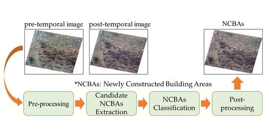
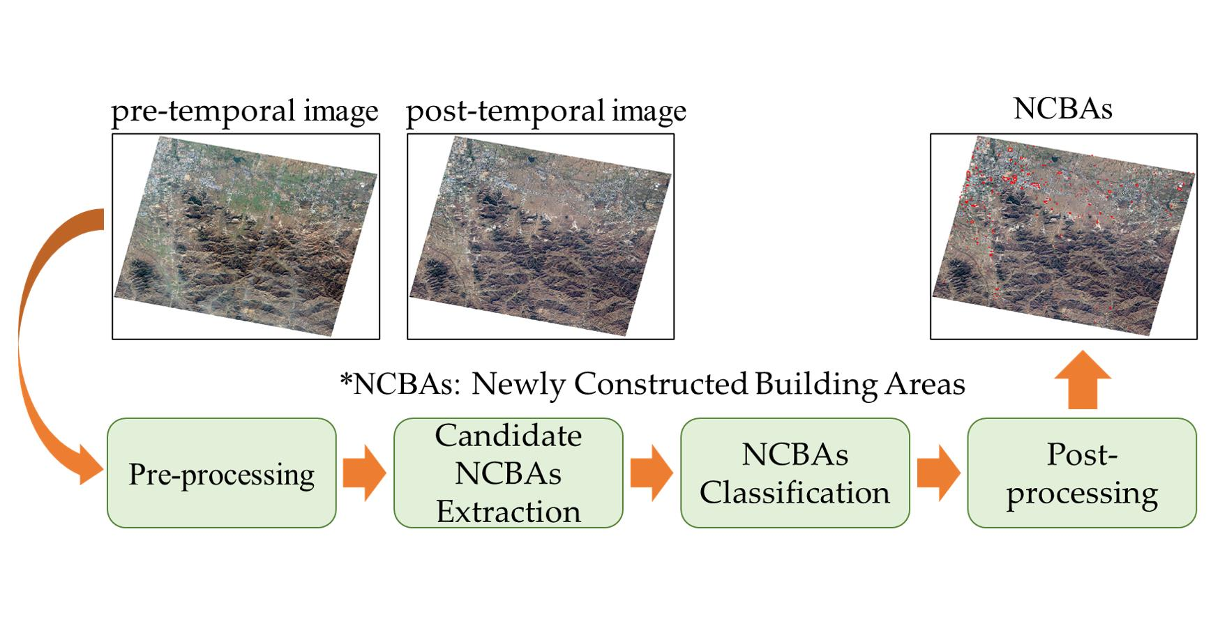
This study aims to automatically detect the existence of NCBAs from bi-temporal high-resolution remote sensing images (GF1 and ZY302 with a resolution of 2 m) based on generalized machine learning (deep learning and support vector machine (SVM)). Accordingly, an automatic change detection for NCBAs method composed of four parts is presented (Figure 1). After pre-processing, the bi-temporal masks obtained by deep learning semantic segmentation are used to extract candidate NCBAs, which are then registered one by one. In the next part, candidate NCBAs would be classified based on priori rules and 14-feature (spectrum, texture, and building probability) SVM classifier. Finally, NCBAs vectors are obtained by post-processing steps such as contour detection, convex hull processing, and vectorization. The major contributions of this study can be summarized as follows:

• The strategy of area registration for NCBAs is proposed to reduce the amount of processed data and improve registration efficiency.
• Combining prior rules (with texture and building probability features) and SVM classifier (with spectrum, texture, and building probability features), this method innovatively divides NCBAs into high, medium, and low confidence levels.
• The vector boundaries of each NCBAs are obtained through post-processing. Area-based accuracy assessment method is adopted to evaluate the vector results of NCBAs obtained by this method.
• The study offers certain insights into change detection of high-resolution remote sensing images based on machine learning for NCBAs.

The rest of this paper is organized as follows. Section 2 introduces related works. Methodology of this paper is detailed in Section 3. Section 4 presents experimental results. The performance of this method is discussed in Section 5. Finally, Section 6 concludes this paper.

2. Related Works

Change Detection: Broadly speaking, pixel-based method and object-based method are the two major categories of change detection methods presented in relevant papers [6,10,11]. Taking pixels as the smallest unit of processing, pixel-based methods detect changes merely through spectral characteristics of pixels, ignoring the spatial context [5,6,12]. As shown in [13,14,15,16,17,18,19,20,21], many researchers have proposed pixel-based change detection methods, yet they are not really suitable for change detection of high-resolution images due to difficult modeling of context information and easy introduction of salt-and-pepper noise [6,20,22,23]. Taking object as the smallest processing unit, object-based methods synthetically adopt information such as context, texture and shape, freeing from disturbance of spatial resolution. Therefore, object-based methods are widely used in change detection, such as [23,24,25,26,27]. However, the detection results of object-based methods depend largely on the result of object segmentation [28]. As deep learning semantic segmentation technology proceeds, segmentation accuracy and efficiency have been greatly improved; therefore, this study mainly uses object-based approach for change detection based on building segmentation results.

Data Pre-processing: Remote sensing images have to be pre-processed before change detection. Common pre-processing methods include radiometric correction, atmospheric correction, and geometric correction. According to Zhu et al. (2017) [29], geometric correction is unnecessary if only L1T Landsat images with good geometric positions were used in change detection tasks. Before change detection, orthorectification, radiation correction and normalization by histogram matching method were performed to ZY3 by Huang et al. (2020) [3]. Song et al. (2001) [30] argued that atmospheric correction is necessary when multi-temporal or multi-sensory images are used in change detection tasks. However, comparing Matched digital counts (DNs), Matched reflections (full radiometric correction and matching), and No pre-processing, Collins et al. (1996) [31] concluded that no evidence shows that Matched reflections performs better than other simple methods during detection. The change detection method proposed in this paper selects fusion, orthorectification, and color-consistency for pre-processing, as detailed in Section 3.1.

Deep Learning Building Semantic Segmentation: Having been successfully applied to image segmentation, Fully convolutional networks (FCN) [32] and encoding-decoding structure networks [33,34,35] perform slightly better than traditional computer vision methods [36]. Fusing low-level information is usually applied to supplement the detailed information lost by down sampling and pooling in FCN [32], Unet [33] and DeepLabV3+ [35], and hole convolution to expand the receptive field and extract denser features without additional parameters in DeepLabV3 [37] and DeepLabV3+ [35]. Deep convolutional neural networks (CNNs) currently share the best accuracy on multiple building semantic segmentation tasks. Consequently, a wide range of studies have employed deep learning semantic segmentation technology to extract building information; for example, [38,39,40,41,42] have improved the strength of classical models, and the improved models were subsequently proved to be more suitable for building segmentation. This study employs classic Resnet+FPN network to extract building information, as described in Section 3.2.

Image Registration: Fake changes are mostly caused by image registration errors, which should thus be avoided [6]. Dai et al. (1998) [43] found that when the registration accuracy is higher than 0.2 pixels, the change detection accuracy would not be lower than 90%. Shi et al. (2013) [44] identified that the commission error caused by the registration error of 0–1 pixels is almost always within 1 pixel of the edge, regardless of image resolution. Featuring invariance of rotation, scale scaling and luminance variation, SIFT [45,46] algorithm could detect key points in scale space and determine the scale and location of key points. SIFT algorithm was then optimized by Pca-SIFT [47] and SURF [48]. Refs. [49,50,51] were studied regarding registration in change detection tasks. As an important part of change detection, global image registration is usually performed during Data Pre-processing. In this study, area registration was carried out on each candidate NCBAs, realizing high registration accuracy of each area and high efficiency. See Section 3.2 for details.

Change Areas Classification: As one feature is inadequate for change detection and may result in missing or false detection, the object-oriented multi-feature fusion method (in which feature vectors and classifiers are used to determine changes and non-changes) is widely used for change detection. Usually, spectrum and texture features are included in feature vectors [52,53,54,55,56]. Spectrum features are usually measured by the mean, variance and ratio of bands, and other indexes or statistical values. Texture features are usually composed of GLDM (Gray Level Dependence Matrix), filtering and morphological operators. Tan et al. (2019) [52] integrated spectrum, statistical texture, morphological and Gabor features, Wang et al. (2018) [53] synthesized spectrum, shape and texture features, and He et al. (2009) [54] put forward differential Histogram of Oriented Gradient (dHOG) feature for classification in change detection. SVM, K-Nearest Neighbor (KNN), Random Forest (RF), and Multilayer Perceptron (MP) are commonly used machine learning classifiers [52]. Wu et al. (2012) [55] and Volpi et al. (2011) [56] trained SVM for classification. Tan et al. (2019) [52] constructed Dempster–Shafer (D-S) classifier by using SVM, KNN and extra-trees. Wang et al. (2018) [53] adopted KNN, SVM, extremum learning machine, and RF for non-linear classification, and then integrated the results of multiple classifiers by an integration rule called weighted voting. In this study, prior rules and 14-feature SVM classifier are combined to classify change areas, as presented in Section 3.1.

Result Form: The results of the above change detection methods are basically change pixels rather than vectors. In this study, NCBAs are obtained through connected-component analysis based on newly constructed building pixels (NCBPs), and further processed in post-processing by graphical method (See Section 3.4).

3. Methodology and Methods

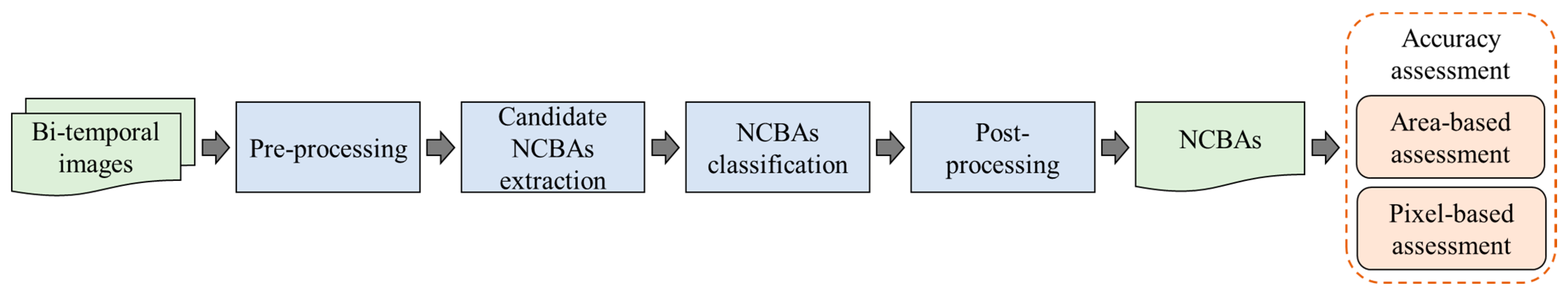
The refined change detection method for monitoring bi-temporal dynamics of NCBAs consists of four parts: (1) pre-processing; (2) candidate NCBAs extraction; (3) NCBAs classification; (4) post-processing, and final accuracy assessment. The details of each part are presented below.

3.1. Pre-Processing

In this paper, pre-processing of bi-temporal images consists of two steps: (1) data processing, and (2) color-consistency processing. The details of each step are described as follows:

(1) Data processing: The spatial details of multi-spectral images were sharpened by panchromatic images to generate fused images, which were subsequently orthographical corrected by RPC model and then mosaicked if necessary. The algorithms used above were realized programmatically based on GDAL library [57] with default parameters.

(2) Color-consistency processing: The differences of satellite sensors, shooting factors and shooting time may lead to color differences among images. This may affect classification of change areas, resulting in relatively large deviations in change detection results. Therefore, to keep the hue of bi-temporal images consistent, histogram matching method was adopted by this study for color-consistency processing [58]. Match the histogram of an image to the histogram of another image by band, so that the two images have similar histogram distribution in their corresponding band, and finally achieve color-consistency.

3.2. Candidate NCBAs Extraction

Candidate NCBAs was extracted by 3 steps: (1) semantic segmentation; (2) candidate NCBAs extraction; and (3) area registration.

(1) Semantic segmentation: The neural network of Resnet50+FPN was chosen for building segmentation. With residual module, Resnet can effectively alleviate network degradation as the number of layers increases [59]. FPN [60] can optimize the performance of small-scale building segmentation and improve detail extraction by fusing shallow and deep feature maps. This study takes fused multi-spectral images (including red, green, blue, and infrared bands) collected by remote sensing satellites and manually labeled building images as training data, which was randomly augmented by Gamma Transform, Saturation Transform, Contrast Transform, Defocusing Blurring, Sharpening, Random Rotation, and Random Clipping during training. The above algorithms for augmentation were all programmed based on Python and then embedded in PyTorch for training of building segmentation. Subsequently, the building and non-building probability of the images were predicted based on the final weight, and then the building mask of the images were obtained by the binary classification function, such as argmax.

(2) Candidate NCBAs extraction: Bi-temporal building masks were dilated and eroded morphologically to eliminate the small cavities inside the building masks. NCBPs were obtained when the pixel value of pre-temporal building mask is 0 while that of post-temporal building mask is 1, as described in Formula (1).

Where $NCBPs$ is the result of candidate NCBPs, $Mask1$ and $Mask2$ pre-temporal and post-temporal building masks, $x$,$y$ the row and column number, and $J(a,b)$ a judging function. In addition, according to provisions by the Ministry of Natural Resources of the People’s Republic of China, the minimum mapping unit is set as $400 {\mathrm{m}}^2$ [61], indicating that NCBAs less than $400 {\mathrm{m}}^2$ are not considered. Candidate NCBAs were finally acquired through connected-component analysis based on NCBPs.

$$NCBPs=J\left(Mask1(x,y) , 0\right)\times J\left(Mask2(x,y) , 1\right)$$

(1)

$$J(a,b)=\{\begin{array}{ll}1 \hfill & if(a==b)\hfill \\ 0\hfill & other\hfill \end{array}$$

(2)

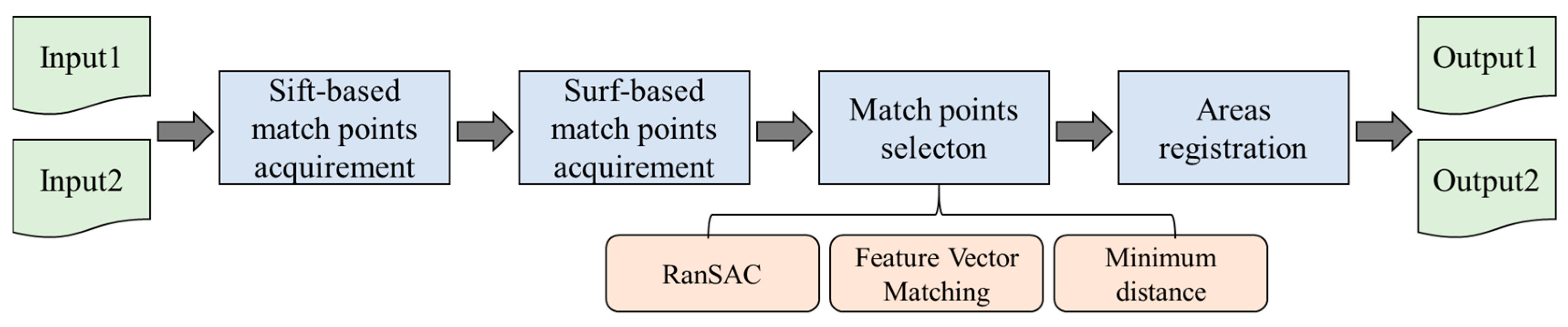
(3) Areas registration: Local translation distortion caused by terrain, shooting angle and other reasons still exists after RPC correction. To solve this problem, SIFT and SURF algorithms were combined to refine registration of NCBAs in this paper. As shown in Figure 2, after matching points are obtained by SIFT and SURF, the rules of RanSAC [62], Feature Vector Matching and Minimum Distance are used to select true matching points and eliminate false ones. The algorithms mentioned above were realized based on OpenCV with default parameters. Integrating SIFT’s feature stability and SURF’s feature point extraction ability of edge smooth target, the areas registration in this study shares high robust, wide application, and small vulnerability to terrain diversity.

3.3. NCBAs Classification

Based on 14 features, candidate NCBAs were classified into high, medium, and low confidence by rules and SVM combined classifier. In addition to spectrum and texture features, probability features were also selected as feature vectors. The process of candidate NCBAs classification is composed of 2 steps: (1) feature vector computation; (2) NCBAs confidence classification. The details of each step are described as follows:

(1) Feature vectors computation: As shown in

Table 1. Feature Selection Results.

Types	Selected Features
spectrum	Former Gray Mean (FGM), Latter Gray Mean (LGM), Former Gray Var (FGV), Latter Gray Var (LGV), Difference Gray Mean (DGM), Difference Gray Var (DGV)
probability	Former Probability Mean (FPM), Latter Probability Mean (LPM), Former Probability Var (FPV), Latter Probability Var (LPV), Difference Probability Mean (DPM), Difference Probability Var (DPV)
texture	SSIM Mean (SSM) and SSIM Var (SSV)

, 14 features of NCBAs were selected, including Former Gray Mean (FGM), Latter Gray Mean (LGM), Former Gray Var (FGV), Latter Gray Var (LGV), Former Prob Mean (FPM), Latter Probability Mean (LPM), Former Probability Var (FPV), Latter Probability Var (LPV), Difference Gray Mean (DGM), Difference Gray Var (DGV), Difference Probability Mean (DPM), Difference Probability Var (DPV), SSIM Mean (SSM), and SSIM Var (SSV). FGM, LGM, FGV, and LGV reflect spectrum features of bi-temporal images, while differential features of spectrum among bi-temporal images are represented by DGM and DGV. Closer values of FGM and LGM and lower values of DGM entail greater similarity of spectrum pixel value, and closer values of FGV and LGV and lower values of DGV entail greater similarity of spectrum distribution of pixel value. FPM, LPM, FPV, and LPV represent building probability features of bi-temporal images, while differential features of building probability among bi-temporal images are represented by DPM and DPV. Closer values of FPM and LPM and lower values of DPM entail greater similarity of building probability, and closer values of FPV and LPV and lower values of DPV entail greater similarity of building probability distribution. SSM and SSV represent texture features among bi-temporal images, i.e., higher value of SSM and lower value of SSV entail smaller difference in structure. In conclusion, NCBAs features can be described by 14 features selected from three aspects: spectrum, building probability and texture. The feature calculation process is detailed below.

Formula (3) is applied to transform multichannel images into single-channel gray images, and Formulas (5) and (6) to calculate values of FGM, LGM, FGV, and LGV of NCBAs. Bi-temporal gray difference is calculated by Formula (4), and then DGM and DGV values by Formulas (5) and (6).

Based on the results of building probability, FPM, LPM, FPV, LPV, DPM, and DPV are calculated by Formulas (5) and (6), while differential building probability by Formula (4).

The SSIM Index Mapping Matrix [63] in each window was calculated based on the bi-temporal images when the gauss weighted function with a radius of 11 and standard deviation of 1.5 was taken as weighted window, and values of SSM and SSV were then calculated by Formulas (5) and (6).

$$Gray(x,y)=0.114\times B(x,y)+0.587\times G(x,y)+0.299\times R(x,y),$$

(3)

$$Diff(x,y)=I_F(x,y)-I_L(x,y),$$

(4)

$$Mean=\frac{1}{MN}{\displaystyle \sum _{x=1}^M{\displaystyle \sum _{y=1}^{N}I(x,y)}},$$

(5)

$$Var=\frac{1}{MN}{\displaystyle \sum _{x=1}^M{\displaystyle \sum _{y=1}^N{(I(x,y)-Mean)}^2}}$$

(6)

where $x$,$y$ represent the row and column number, $B(x,y)$, $G(x,y)$ and $R(x,y)$ pixel values of Blue, Green, Red (Band1-3 in GF1 and ZY302) in $(x,y)$, $Gray(x,y)$ the gray images, $Diff(x,y)$ the differential results among bi-temporal images, $I_F(x,y)$ pre-temporal images, $I_L(x,y)$ post-temporal images, $Mean$ mean of input, $Var$ variance of input, $M$ and $N$ the width and height of input images, and $I(x,y)$ pixel value of input.

(2) NCBAs confidence classification: The feature vectors of the selected samples were calculated according to the above method, and true NCBAs samples were labeled as 1, while false NCBAs as −1. L2-Regularized Linear SVM classifier for binary classification was adopted for training, until tolerance was less than 1 × 10⁻⁵. The scores given by SVM to candidate NCBAs were −1 and 1. Specifically, scores greater than 0 indicate true NCBA and those less than 0 indicate false NCBA by SVM classifier. Additionally, prior knowledge exists in this study before SVM. Lower value of SSM indicates larger difference in texture structure of a NCBA in bi-temporal images. Moreover, higher value of $abs(DPM)$ possibly indicates larger difference in building probability of a NCBA among bi-temporal images. Lower SSM value combined with higher $abs(DPM)$ value increases the probability of true NCBA. Therefore, a combined classifier of rules and SVM was applied to classify NCBAs into high, medium and low confidence in this study, according to Formula (7). With relatively large thresholds and wide range, NCBAs failing to meet the prior rules would directly be judged as $Valu{e}_{ncba}$1. Within the scope of prior rules, according to SVM, if the score of a NCBA is greater than 0, then this NCBA would be judged as $Valu{e}_{ncba}$3, while that less than 0 as $Valu{e}_{ncba}$2.

$$Valu{e}_{ncba}=\{\begin{array}{l}3,if (SSM\le th\_ssm and abs(DPM)\ge th\_dpm and Score>0)\hfill \\ 2,if (SSM\le th\_ssm and abs(DPM)\ge th\_dpm and Score<0)\hfill \\ 1,others\hfill \end{array}$$

(7)

where $SSM$ and $DPM$ stand for the values of SSM and DPM of a NCBA, $th\_ssm$ and $th\_dpm$ thresholds of SSM and DPM, $abs()$ absolute value function, $Score$ score of SVM classifier, and $Valu{e}_{ncba}$ of 3, 2, and 1 high, medium, and low confidence.

3.4. Post-Processing

NCBAs were further processed by three steps: (1) contour detection, (2) convex hull processing, and (3) vectorization. The details of each step are described below:

(1) Contour detection: Detect contour of each NCBA and save all the continuous contour points on the contour boundary.

(2) Convex hull processing: Obtain convex hull range of NCBAs based on the continuous contour points on the contour boundary.

(3) Vectorization: Vectorize the convex hull obtained in the previous step and get the final vector results of NCBAs with classified attribute of 3, 2, and 1.

3.5. Accuracy Assessment

According to the manually delineated NCBAs, area-based and pixel-based assessment including PA (Pixel Accuracy), Recall, and F1 was conducted to evaluate the results.

$$PA=\frac{TP}{TP+FP},$$

(8)

$$Recall=\frac{TP}{TP+FN},$$

(9)

$$F1=\frac{2\times PA\times \mathrm{Re}call}{PA+\mathrm{Re}call}$$

(10)

(1) Area-based assessment: Algorithmic NCBAs intersecting true NCBAs are considered as true algorithmic NCBAs $T{P}_a$ (True Positive Areas), otherwise as false algorithmic NCBAs $F{P}_a$ (False Positive Areas). True NCBAs which does not intersect algorithmic NCBAs are considered as missing algorithmic NCBAs $F{N}_a$ (False Negative Areas). $P{A}_a$, $\mathrm{Re}cal{l}_a$ and $F{1}_a$ were calculated according to Formulas (8)–(10).

(2) Pixel-based assessment: $T{P}_p$ (True Positive Pixels) denotes the number of pixels correctly classified as NCBAs pixels by the algorithm, $F{P}_p$ (False Positive Pixels) the number of non-NCBAs pixels incorrectly classified as NCBAs pixels, and $F{N}_p$ (False Negative Pixels) the number of pixels of NCBAs incorrectly classified as non-NCBAs pixels. $P{A}_p$, $\mathrm{Re}cal{l}_p$ and $F{1}_p$ can be calculated according to Formulas (8)–(10).

4. Experiment and Result

4.1. Experimental Data

4.1.1. Image Data and Labeled NCBAs

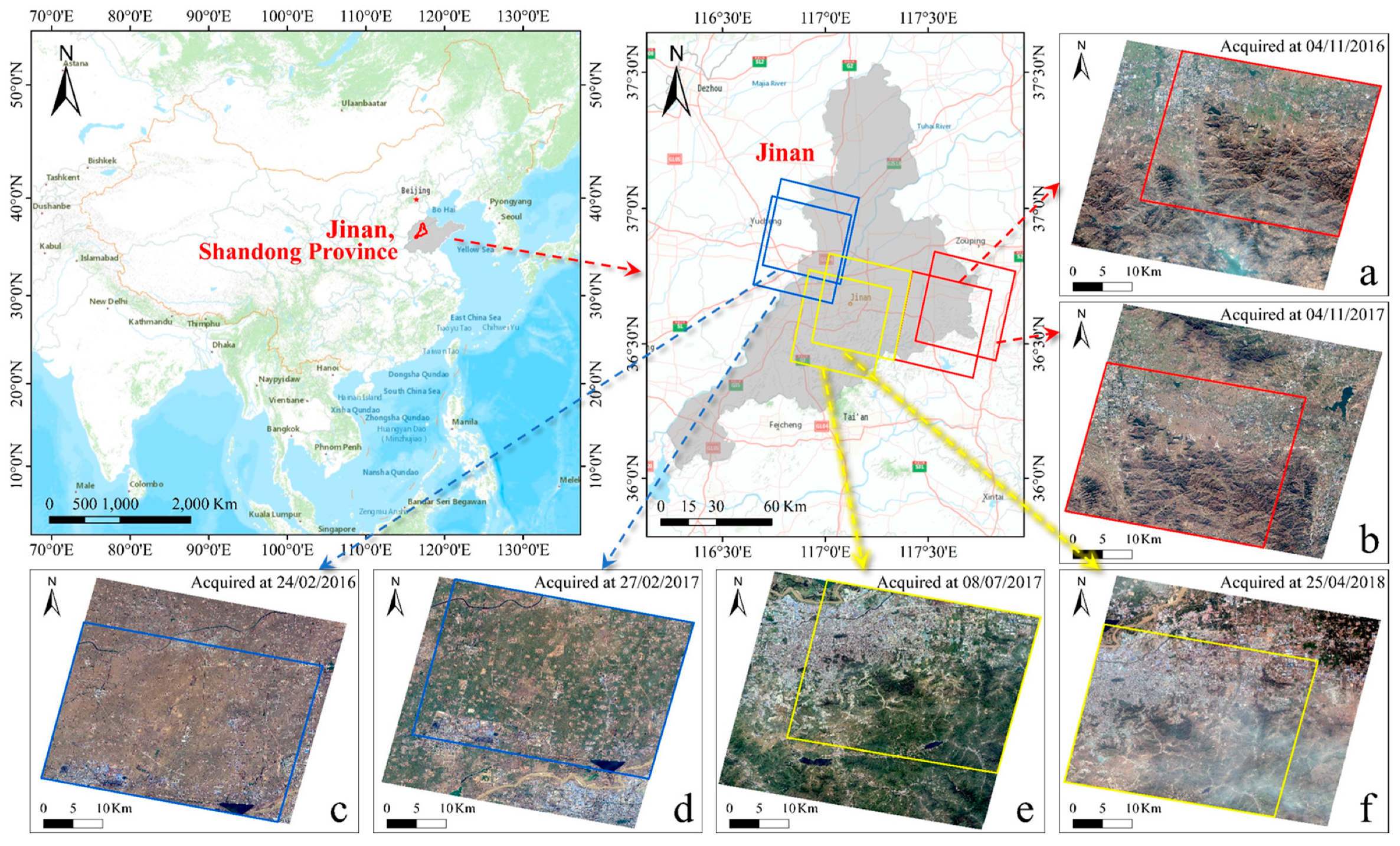
The PMS camera carried by the GF-1 satellite can capture panchromatic images with a resolution of 2 m and multispectral images (including blue, green, red, and near-infrared bands) with a resolution of 8 m. The experimental data (from scientific research data) consists of three groups of GF1 remote sensing images covering parts of Jinan, Shandong Province, and the resolution reaches 2 m after data pre-processing, as shown in Figure 3. The pre-temporal images were acquired on 4 November 2016 (group 1), 24 February 2016 (group 2), and 8 July 2017 (group 3), and the post-temporal images on 4 November 2017 (group 1), 27 February 2017 (group2), and 25 April 2018 (group 3).

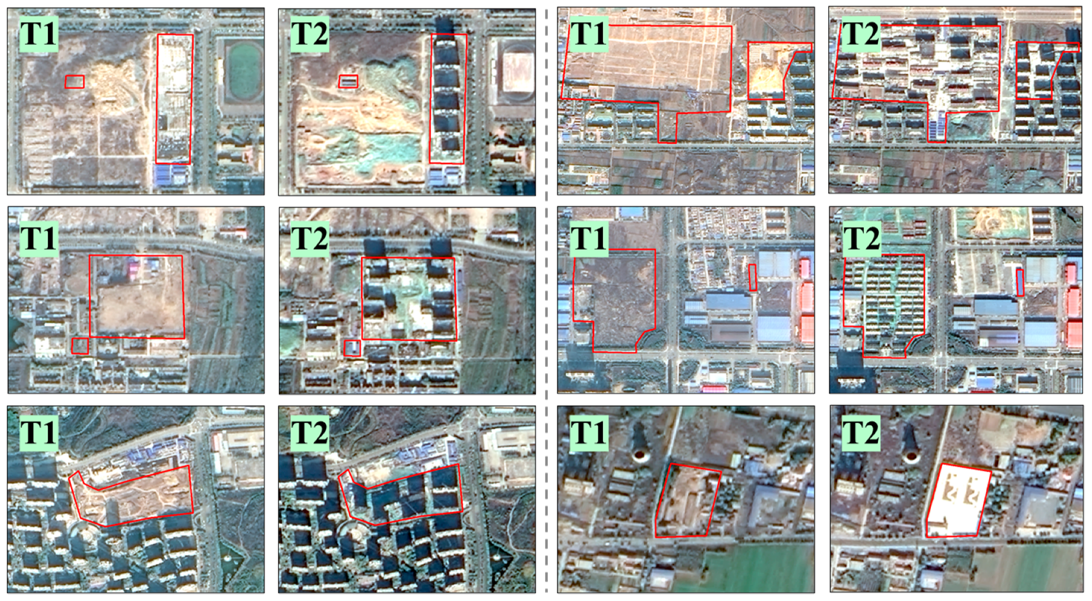
The labeled NCBAs were manually drawn after field investigation, mainly dealing with the building areas developed from non-building areas such as bare land, dig land, and cultivated land, as shown in Figure 4.

4.1.2. Dataset of Building Segmentation

In the step of building semantic segmentation, the images for training were from two sensors, GF1 and ZY302. 14,644 pieces of 500 ∗ 500 fusion images were included in our dataset, covering about 14,000 square kilometers, that is, nine cities in China (Beijing, Tianjin, Zhenjiang, Wuhan, Xuzhou, Suizhou, Ezhou, Jiaozhou, and Shijiazhuang). The labeled build-up area was obtained manually after field investigation, mainly including office building area, commercial area, residential area, scattered village area, and other non-building areas.

4.1.3. Dataset of SVM Classifier

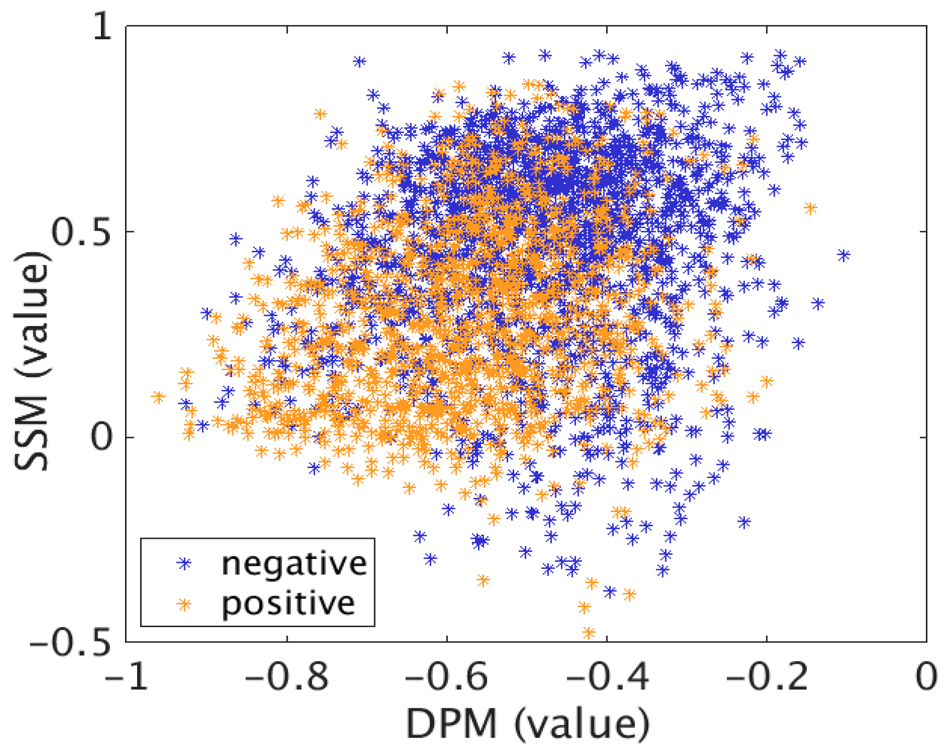
The feature vectors of 1173 true NCBAs and 1797 false NCBAs from two satellites (GF1 and ZY302) were selected as training data for SVM classifier, and the number of true NCBAs was doubled during training. The distribution of training data is shown in Figure 5.

4.2. Experiment Results

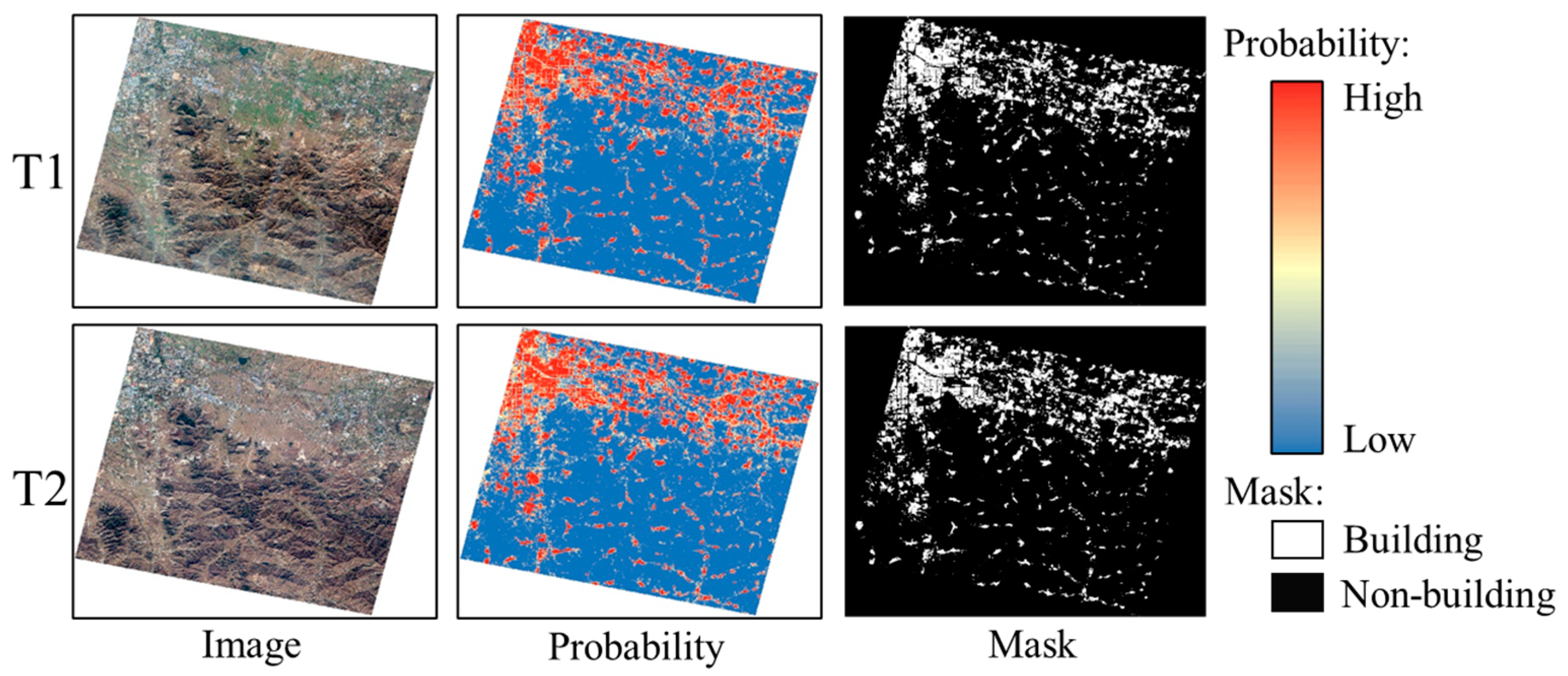
4.2.1. Building Segmentation

After 200 epochs of training, the Recall of the final building segmentation model reaches 88.94%, and Precision 90.32%. To improve efficiency, only the common area of bi-temporal images was selected for processing in the following experiment. The bi-temporal results (for group 1) of building probability and mask of the common area are shown in Figure 6.

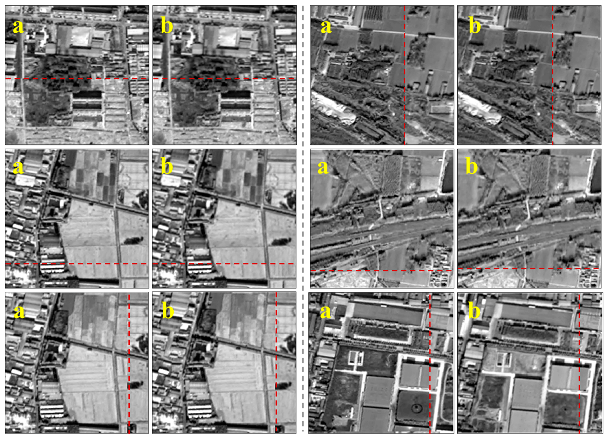
4.2.2. Area Registration

According to the rule of expanding 100 pixels around the image, image patches of candidate NCBAs were captured and registered by the above algorithm. As shown in Figure 7, the error of areas registration is within 0.5 pixels.

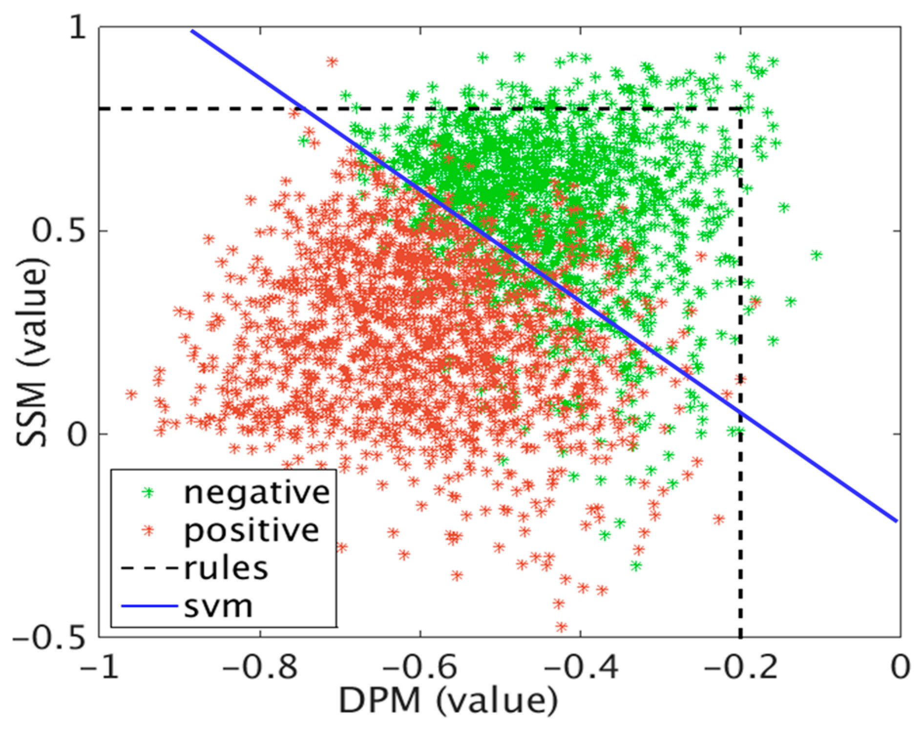
4.2.3. Rules and SVM Classifier

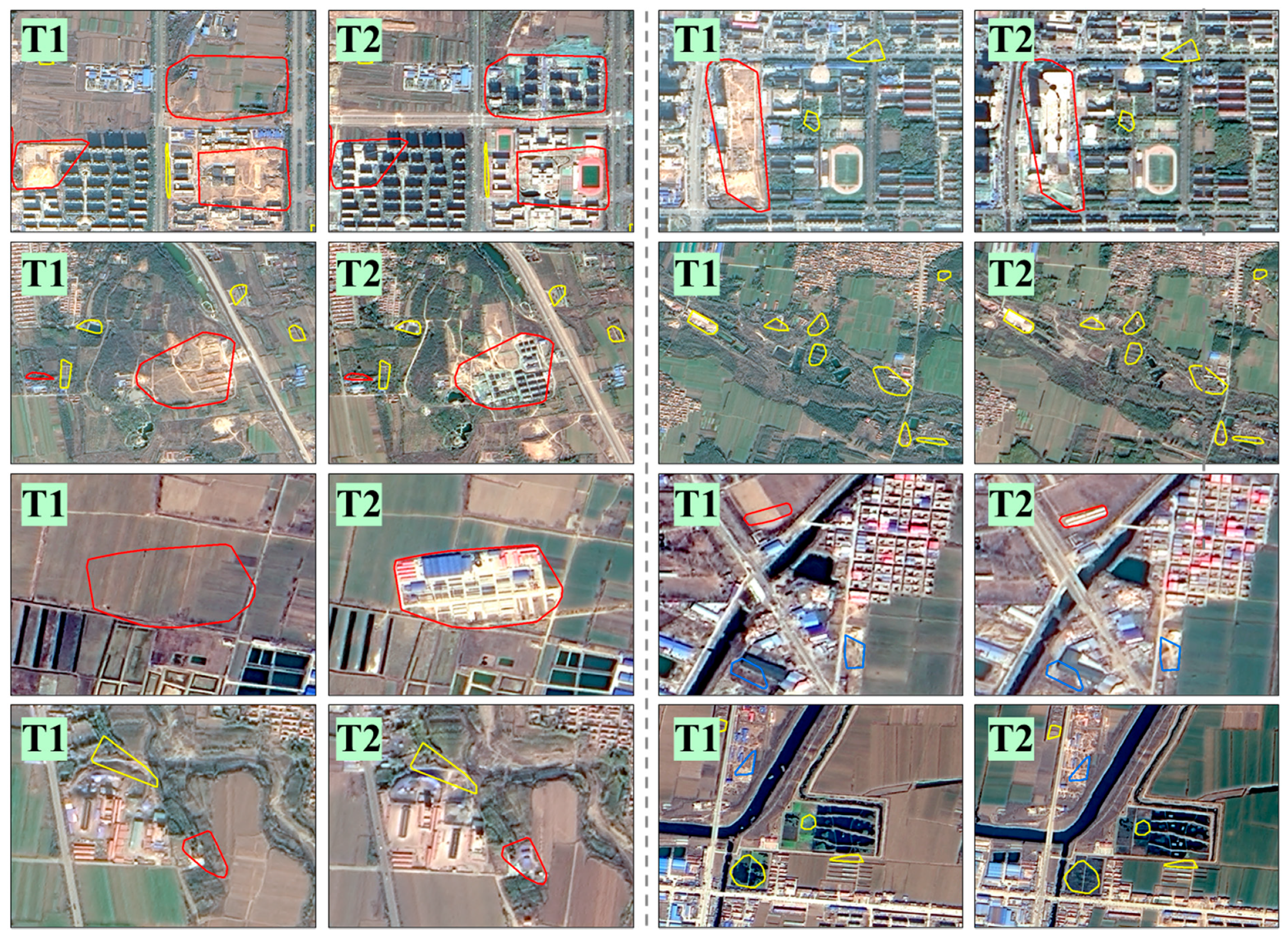
Figure 8 shows the classification result of training data by SVM classifier. The Recall reaches 73.91% and overall Accuracy 70.65%. This study set $th\_ssm$ as 0.8 and $th\_dpm$ 0.2. With relatively large threshold range, a small number of NCBAs were classified as low confidence, and most NCBAs as high and medium confidence. Figure 9 shows the detection and classification results of randomly intercepted NCBAs. Areas surrounded by red polygons are basically true NCBAs, while by yellow and blue polygons are basically false NCBAs.

4.3. Accuracy Assessment

Table 2. Results of accuracy assessment. PA stands for Pixel Accuracy.

Confidence	Group	Area-Based Assessment			Pixel-Based Assessment
		PA	Recall	F1	PA	Recall	F1
High	1	93.45%	73.54%	82.31%	96.46%	89.41%	92.80%
	2	90.73%	73.10%	80.97%	91.91%	89.45%	90.66%
	3	79.21%	84.72%	81.87%	86.69%	93.64%	90.03%
	mean	87.80%	77.12%	81.72%	91.69%	90.83%	91.17%
High-medium	1	41.42%	78.01%	54.11%	67.49%	89.79%	77.06%
	2	60.31%	76.62%	67.49%	72.51%	89.61%	80.16%
	3	35.13%	91.85%	50.82%	56.87%	93.85%	70.82%
	mean	45.62%	82.16%	57.48%	65.62%	91.08%	76.01%
High-medium-low	1	38.27%	79.04%	51.57%	67.56%	90.04%	77.19%
	2	57.81%	77.18%	66.10%	70.55%	89.94%	79.08%
	3	35.09%	97.28%	51.58%	55.79%	93.89%	69.99%
	mean	43.72%	84.50%	56.42%	64.63%	91.29%	75.42%

presents the results of accuracy assessment under three cases. High confidence expresses NCBAs with $Valu{e}_{ncba}$3, High-medium confidence NCBAs with $Valu{e}_{ncba}$3 and 2, and High-medium-low confidence all the NCBAs with $Valu{e}_{ncba}$3, 2, and 1. NCBAs satisfying rules were classified into High-medium confidence, and those not satisfying rules low confidence. Therefore, NCBAs of High-medium confidence is merely the results of rule classification.

The statistical values of area-based assessment are lower than those of pixel-based assessment, indicating that small NCBAs are prone to be misjudged by this method. Small-area NCBAs covering fewer pixels exert more influence on area-based assessment than pixel-based assessment. For example, in 100 true NCBAs of 1000 pixels, 20 small NCBAs occupying 100 pixels are missed; thus, the recall of area-based assessment is 0.8, while that of pixel-based assessment is 0.9. Additionally, in two assessment methods, the PA and F1 of the three groups decrease from High, High-medium, to High-medium-low confidence, while Recall increase.

From High to High-medium confidence, the mean Recall of the two accuracy assessment methods increases by 5.04% and 0.25%, while PA decreases by 42.18% and 26.07%, respectively. The increase of mean Recall for area-based assessment is more obvious than that of pixel-based assessment, indicating that a number of small-area NCBAs may ignored by High confidence. Yet the obviously decreased PA reveals that many NCBAs were over-checked by High-medium confidence, leading to sharply increased FP and correspondingly decreased PA.

Similarly, from High-medium to High-medium-low confidence, the Recall of the two accuracy assessment methods increases by 2.34% and 0.21%, while PA decreases by 1.9% and 0.99%, respectively. This may indicate that a tiny part of small-area NCBAs were omitted by High-medium confidence. Yet the decrease of PA and F1 and increase of Recall appear slow in both area-based and pixel-based assessments, reflecting that most candidate NCBAs satisfy prior rules, and could classified into High-medium confidence.

On the whole, NCBAs of High confidence records the best balance of PA and Recall, and the highest F1 (81.72% and 91.17%), while High-medium confidence and High-medium-low confidence lead to slightly increased Recall yet significantly decreased PA. Therefore, to balance PA and Recall and achieve favorable results, only NCBAs of High confidence are considered to be the final detection result by this method.

5. Discussions

The applicability of this method to ZY302 is verified through two groups of experiments. Subsequently, registration strategy and NCBAs classification are presented in Section 5.2 and Section 5.3. In addition, error types and sources for detecting NCBAs by this method are briefly analyzed in Section 5.4. Finally, the contribution of this method is briefly explained.

5.1. Application

The images obtained by ZY302 include panchromatic images with a resolution of 2.1 m and multispectral images making up of blue, green, red, and near-infrared bands with a resolution of 6 m. The ZY302 experimental images (from scientific research data) of Xi’an and Kunming were selected for accuracy assessment and verification of the applicability of the method on ZY302. Obtained on 22 March 2018 and 4 March 2020, the bi-temporal images of Xi’an cover the main urban area and part of suburb in Xi’an. Obtained on 31 March 2018 and 11 May 2020, the bi-temporal images of Kunming cover the central city and surrounding mountainous areas. It can be seen from

Table 3. Accuracy assessment for Xi’an and Kunming.

City	Area-Based Assessment			Pixel-Based Assessment
	PA	Recall	F1	PA	Recall	F1
Xi’an	92.18%	72.77%	81.29%	92.15%	89.31%	90.70%
Kunming	94.90%	72.52%	82.22%	97.57%	87.20%	92.10%
mean	93.49%	72.65%	81.76%	94.86%	88.25%	91.40%

that the mean score of F1 for area-based assessment reaches 81.76%, and pixel-based assessment 91.40%. Missed detection of rebuilt NCBAs in urban areas results in relatively low Recall.

The dataset of building segmentation and SVM classifier deal with two satellites (GF1 and ZY302); that is, the building segmentation model and SVM classification model are both trained based on the data from GF1 and ZY302. It can be observed from the results (F1 of pixel-based assessment > 90%) of three sets of GF1 (Section 4.3) and two sets of ZY302 that this method is adaptable to the data of GF1 and ZY302 and can provide a new idea for change detection of multi-sensor images.

5.2. Areas Registration

According to the rule of expanding 100 pixels, the range of each candidate NCBA was intercepted, and area registration was performed instead of full image registration. Only suspected NCBAs were registered, while other areas without candidate NCBAs were skipped. This strategy substantially reduces the amount of data that needs to be processed during registration, shortens the process of selecting matching points of uninterested areas, and improves the efficiency of registration. Meanwhile, registration of small area can also curtail registration conflicts among matching points and improve registration accuracy.

5.3. NCBAs Classification

5.3.1. Single Use of 14-Feature SVM

As shown in

Table 4. Accuracy assessments for single use of 14-feature SVM.

Classifier	Group	Area-Based Assessment			Pixel-Based Assessment
		PA	Recall	F1	PA	Recall	F1
Single use of 14-feature SVM	1	88.76%	75.95%	81.85%	93.42%	89.71%	91.53%
	2	86.99%	75.35%	80.75%	89.13%	89.46%	89.30%
	3	63.02%	85.06%	72.40%	80.37%	94.21%	86.74%
	mean	79.59%	78.79%	78.34%	87.64%	91.13%	89.19%

, we compared the accuracy assessments for single use of 14-feature SVM and combination use of rules and 14-feature SVM (Table 2 High confidence). It can be seen that single use of SVM classifier could increase the mean Recall of area-based assessment and pixel-based assessment by 1.67% and 0.30%, but decrease the mean PA by 8.21% and 4.05%, and F1 by 3.38% and 1.98%, respectively. Therefore, the single use of SVM classifier could reduce missed detection yet increase false detection.

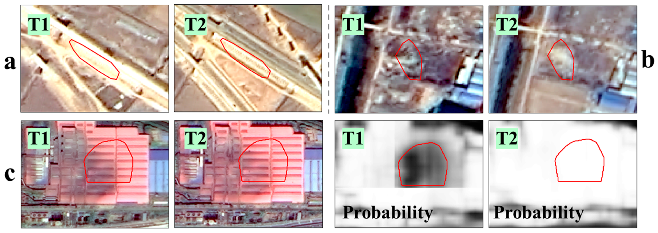
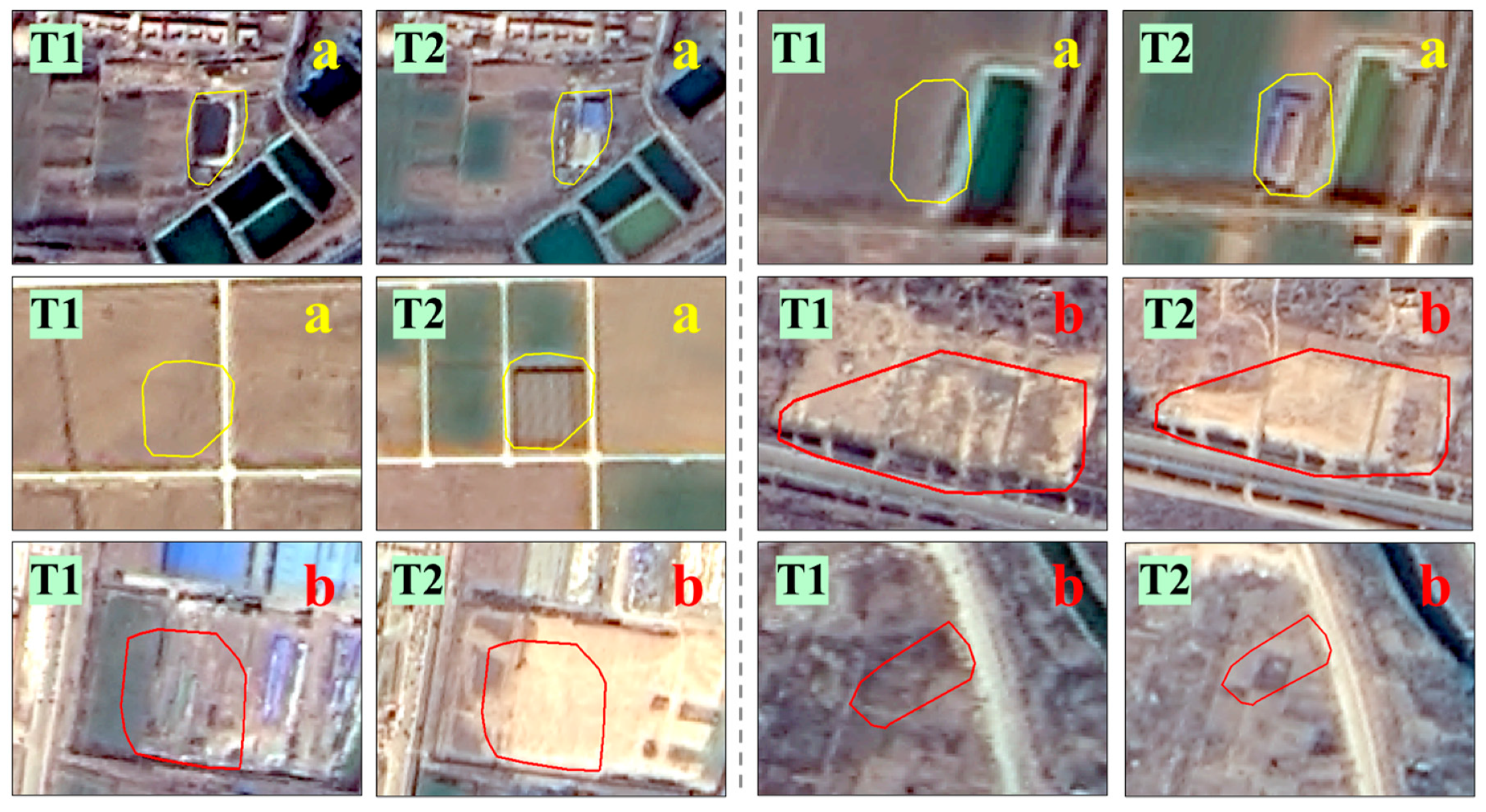
Figure 10 displays NCBAs failing to meet the rules yet are greater than 0 in SVM score. The texture features of (a) and (b) change, but the value of DPM fails to meet the threshold. The overexposure of pre-temporal image of (a) leads to loss of texture details, thus the value of SSM is lower than the actual value. The red circled area in (b) is covered by vegetation in pre-temporal images yet is bare in post-temporal images, leading to lower SSM value too. In (c), due to the deviation of building probability in the pre-temporal image, higher DPM value than actual value occurs, resulting in DPM meeting the threshold. However, SSM value cannot reach the threshold, resulting in failure to meet the rules. To sum up, DPM could decrease the false detection caused by pseudo texture changes in high-resolution images, and SSM could reduce the false detection caused by building segmentation errors. Therefore, the rules combining SSM and DPM can improve detection accuracy.

5.3.2. Single Use of 8-Feature SVM

Eight non-probability features (FGM, LGM, FGV, LGV, DGM, DGV, SSM, and SSV) were also employed to train SVM classifier for candidate NCBAs classification. The Recall reaches 74.42% and overall Accuracy 68.53%. Compared with the accuracy assessment of 14-feature SVM classifier (Table 4), the values of PA, Recall, and F1 are all decreased significantly in the accuracy assessments of 8-feature SVM classifier (

Table 5. Accuracy assessment for 8-feature SVM classifier.

Classification	Group	Area-Based Assessment			Pixel-Based Assessment
		PA	Recall	F1	PA	Recall	F1
Single use of 8-feature SVM	1	79.61%	69.76%	74.36%	91.45%	84.11%	87.63%
	2	78.44%	72.25%	75.22%	85.29%	87.16%	86.21%
	3	60.78%	81.83%	69.75%	79.94%	59.22%	68.04%
	mean	72.94%	74.62%	73.11%	85.56%	76.83%	80.63%

). Examples of 8-feature SVM classifier scoring less than 0 and 14-feature one scoring greater than 0 are shown in Figure 11a. It can be seen that 8-feature SVM classifier may lead to loss of some small-area NCBAs, which account for less pixels and are easily to be dominated by other pixel values in the overall assessment of spectral and texture features of the region, thus mistakenly divided into non-changing area. In addition, examples of 8-feature SVM classifier scoring greater than 0 and 14-feature one scoring less than 0 are shown in Figure 11b. False NCBAs not converting from non-building to building could be incorrectly classified as real NCBAs by 8-features SVM classifier because of changes in texture and spectrum.

5.4. Error Analysis

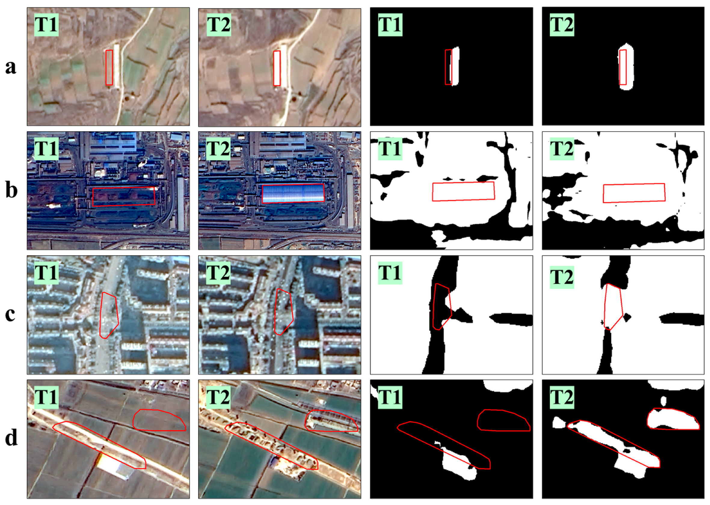
The error types of NCBAs detection are analyzed by examples in Figure 12. As the variation range of building mask shown in (a) is less than $400 {\mathrm{m}}^2$, it was filtered out during candidate NCBAs extraction. The new single building in (b) was also ignored during candidate NCBAs extraction as the bi-temporal masks have regarded it as building. Because of threshold of minimum area and building segmentation problem, the NCBAs in (a) and (b) failed to be detected, resulting in loss of Recall. As shown in (c), the road in the post-temporal image was over-checked, resulting in false NCBAs in candidate NCBAs extraction. Moreover, due to the differences in texture and building probability between bi-temporal images, this false NCBA has passed the test of rules and SVM classifier, and was classified as high confidence finally, leading to over-examination. The manually marked NCBAs do not include the type of land turned into piers, resulting in the NCBA in (d) are counted as an over-checked NCBA in accuracy assessment. Due to the building segmentation errors and limited manually labeled types, the NCBAs in Figure 12c,d failed to be considered as true NCBAs, leading to loss of PA. In conclusion, the detection errors of NCBAs by this method may be caused by limit of minimum area, imprecision and misclassification of building segmentation, and limited manually labeled types.

5.5. Contributions

This study is contributive to NCBAs monitoring in three aspects:

Firstly, the experimental results of Jinan, Xi’an, and Kunming show that the proposed method can achieve high accuracy (the F1 of area-based and pixel-based methods are above 80% and 90%, respectively) in detecting NCBAs. Introduction of deep learning semantic segmentation and machine learning classification algorithms reduces limitations of spectral characteristics of images and weakens the influence of illumination and atmosphere on detection of NCBAs. Correction of image internal distortion widens the application area of the algorithm (such as the mountainous city of Kunming). In addition, the strategy of area registration saves processing time and improves efficiency.

Then, this method can be used for NCBAs detection based on GF1 and ZY302 images. The complementary use of multi-sensor images can effectively increase monitoring frequency and enhance monitoring ability.

Finally, this refined method can be used for change detection of remote sensing images with a resolution of 2 m, providing a new solution for detection of NCBAs in high-resolution images and improving detection precision.

6. Conclusions

To investigate NCBAs monitoring of high-resolution remote sensing images (GF1 and ZY303 images with a resolution of 2 m), this study proposes a refined NCBAs detection method consisting of four parts based on generalized machine learning: (1) Process data by fusion, orthorectification, and color-consistency; (2) Obtain candidate NCBAs by using bi-temporal building masks acquired by deep learning semantic segmentation, and then register these candidate NCBAs one by one; (3) Classify NCBAs into high, medium, and low confidence by combining rules and SVM classifier with 14 features of spectrum, texture and building probability; and (4) Determine the final vectors of NCBAs by post-processing. In addition, area-based and pixel-based assessment methods are integrated to evaluate PA, Recall, and F1 of three experimental groups in Jinan under three cases (High, High-medium, and High-medium-low confidence). Subsequently, the results of accuracy assessments show that although the Recall of NCBAs with High-medium and High-medium-low confidence increases slightly, PA suffers a great loss, resulting in a decrease in F1 value. To balance PA and Recall and achieve favorable results, only NCBAs of High confidence are considered to be the final detection result by this method. For the three groups of GF1 images of Jinan, the mean Recall of the two assessment methods reaches 77.12% and 90.83%, the mean PA 87.80% and 91.69%, and the mean F1 81.72% and 91.17%, respectively. In addition, the scores of F1 for ZY302 images of Xi’an and Kunming are both above 90%, indicating that this proposed method is also applicable to ZY302 satellite.

By adopting the strategy of candidate NCBAs registration, this method avoids low efficiency of full-image registration. In addition, experiments were conducted to verify the accuracy of single use of 14-feature SVM, and that of combination use of rules and SVM. The results show that the single use of SVM could increase the mean Recall of area-based and pixel-based assessment by 1.67% and 0.30% yet decrease the mean PA of the two assessments by 8.21% 4.05%, and F1 by 3.38% and 1.98%, respectively, while combination use of rules and SVM could prevent false NCBAs from being mis-detected as high confidence ones. The experimental results of 8-feature SVM (spectrum and texture features) and 14-feature SVM (spectrum, texture, and building probability features) were also analyzed. The results reveal that the values of PA, Recall, and F1 of 8-feature SVM are lower than those of 14-feature SVM, which could reduce the over-checking caused by changes in land status, and slightly avoid missed inspections of NCBAs in small areas. It is thus proved that introduction of probability features can improve NCBAs classification accuracy.

This paper is contributive to NCBAs detection in three aspects. To begin with, the introduction of machine learning and area registration algorithms expands the scope and conditions of NCBAs detection by this method. Secondly, being well adaptive to both GF1 and ZY302, this method improves NCBAs monitoring ability through complementary use of multi-sensor images. Finally, the algorithm can be used for NCBAs detection in remote sensing images with a resolution of 2 m, providing a new solution for the change detection of high-resolution remote sensing images.

Limitations are inevitable, and this study is no exception. Imprecision of building segmentation caused by image quality and building size may lead to missing and over detection of NCBAs in this study. In the future study, NCBAs errors caused by building segmentation would be prioritized, to reduce the impact of segmentation results on object-based change detection. In addition, a transfer learning mechanism may be introduced to allow this method to be applied to other satellite images. Moreover, we have plans to release our test set in the future, so that NCBAs detection methods can be compared on the same scale.