Article

A Unified Framework for Anomaly Detection of Satellite Images Based on Well-Designed Features and an Artificial Neural Network

1
Beijing Key Laboratory of Digital Media, School of Computer Science and Engineering, Beihang University, Beijing 100191, China
2
China Centre for Resources Satellite Data and Application (CRESDA), Beijing 100094, China
*
Author to whom correspondence should be addressed.
Remote Sens. 2021, 13(8), 1506; https://doi.org/10.3390/rs13081506
Submission received: 4 March 2021 / Revised: 6 April 2021 / Accepted: 12 April 2021 / Published: 14 April 2021

Abstract

:
Nowadays, as the number of remote sensing satellites launched and applied in China has been mounting, relevant institutions’ workload of processing raw satellite images to be distributed to users is also growing. However, due to factors such as extreme atmospheric conditions, diversification of on-board device status, data loss during transmission and algorithm issues of ground systems, defect of image quality is inevitable, including abnormal color, color cast, data missing, obvious stitching line between Charge-Coupled Devices (CCDs), and inconstant radiation values between CCDs. Product application has also been impeded. This study presents a unified framework based on well-designed features an Artificial Neural Network (ANN) to automatically identify defective images. Samples were collected to form the dataset for training and validation, systematic experiments designed to verify the effectiveness of the features, and the optimal network architecture of ANN determined. Moreover, an effective method was proposed to explain the inference of ANN based on local gradient approximation. The recall of our final model reached 81.18% and F1 score 80.13%, verifying the effectiveness of our method.

Graphical Abstract

1. Introduction

1.1. Background and Motivations

Wide space coverage, short revisit period, rich band information, and fine resolution have contributed positively to remote sensing’s extensive applications in many fields such as land inspection, city planning, weather forecasting, hydrological observation, and military reconnaissance [1]. Since China begun to develop its remote sensing satellites in the 1970s, the number of remote sensing satellites, both state-owned and commercial, has exploded [2]. The growing satellite image products make image quality a top priority.
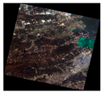
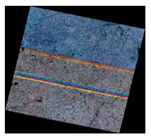
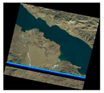
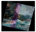
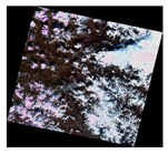
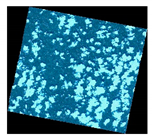
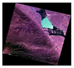
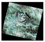
Inevitably, the received raw satellite images may be defective due to various factors, leading to diversified anomalies. For example, the black stripe in Figure 1a may be caused by data loss during signal transmission between satellites and ground stations, the color cast (a superimposed color due to lighting conditions, or the characteristics of a capturing device [3]) in Figure 1b by extreme atmospheric conditions or unsuitable color correction, the stripe with abnormal color in Figure 1c by CCD issues during satellite scanning or imperfect radiation correction during processing of ground system, and the pixels with extreme color in Figure 1d by diverse status of on-board device of the satellite or data processing error such as value type overflow. We here define the anomalies of raw satellite images as unnatural visual performance such as data missing, colorcast, stripe- or block- like noise, extreme color, and so on, which can be caused by system or man-made reasons as illustrated above. Abnormal satellite images are referred to satellite images with anomalies. Such anomalies would significantly affect raw satellite images’ subsequent application. As equipment and technology proceed, the defective rate can be lowered but not eliminated. Therefore, assurance of raw satellite image quality is a long-term task and plays an important role in the whole industry chain of remote sensing.
The most reliable method for quality assurance is manual intervention, yet it is time- and cost-consuming as substantial experienced workers are required to check the images one by one. This study thus presents an ANN model with well-designed features as input, which can automatically score the quality of input satellite images, largely saving time and labor costs.
Basically, the input satellite images are identified as normal or abnormal ones. The challenge lies in the massive and diversified types of anomalies (See Figure 1), that is, the category of “abnormal” contains several subclasses, whose occurrence probability differs, leading to unevenly distributed samples. Besides, the images collected from different satellites (such as GF-1, GF-1B, GF-1C, GF-1D, GF-2, GF-6 and ZY-3-02) share differing image sizes and spectral characteristics, making the images more diverse. Therefore, a unified framework that can uniformly identify different types of input images is necessary.

1.2. Machine Learning and ANN

Performing well in classification and regression issues, machine learning (ML) was introduced. Taken as a subset of artificial intelligence, ML is the study of computer algorithms that improve automatically through experience. ML algorithms build a mathematical model based on sample data (known as “training data”) to make predictions or decisions without explicit programming. There are many ML algorithms that have solid mathematical foundations, such as logistic regression (LR), K nearest neighbor method (KNN), decision tree (DT), random forest algorithm (RF), naïve Bayes algorithms (NB), Support Vector Machine (SVM), ANN, among others [4,5,6,7]. All the above algorithms perform well in solving classification issues under normal circumstances, but we are not sure whether they are suitable for our specific situations. A series of tests were then conducted and ANN was identified as the optimal algorithm (see Section 4.1), perhaps because of its powerful nonlinear fitting ability. It is notable that F1 score, harmonic mean of precision and recall, was prioritized as precision and recall were taken superior to accuracy (samples were unevenly distributed).
Artificial neural network (ANN) is a brain-inspired system that intends to replicate the way of human learning. ANN is composed of an input layer that receives data from outside sources, one or more hidden layers that process the data, and an output layer that provides one or more data points based on the function of the network [8]. ANN uses activation function attached to a neuron that collects the weighted sum of output from the last layer to achieve nonlinear fitting. Such activation functions as Rectified Linear Unit (ReLU) [9], Leaky ReLU, sigmoid, tanh, and swish [10] can be selected. ANN is trained by gradient backward propagation [11], which updates every trainable parameter by adding an item coming from the product of the gradient propagated from loss function and learning rate. After repeated training iterations, the network can acquire the ability of classifying different inputs or reaching an accurate regression value. Composed of tens of hidden layers and thousands of neurons, deep learning has scored dramatic improvement in such fields as computer vision and natural language processing [12]. This study employed shallow ANN instead of deep learning because of the small number of features (less than 30) and samples (less than 10,000), deep learning’s vulnerability to overfitting, and shallow ANN’s saving of time and computing resources.
In this study, the inputs of ANN should be representative features that differ a lot in normal images and abnormal ones, and the output are two nodes that respectively represent normal images and abnormal ones. After a softmax layer, the outputs are normalized to 0~1, standing for the probability of each image belonging to the two categories. In test phase, an image would be identified as abnormal when the probability for abnormal is larger than 0.5, and vice versa.

1.3. Related Works and Novelties and Necessity of the Study

Although we are studying anomaly detection of satellite images, considering the anomalies as we define and illustrate above, the problem is more like image quality assessment (IQA). Many researchers have studied IQA, which can be divided into three types: full-reference IQA, reduced-reference IQA, and no-reference IQA (reference means reference images without distortions) [13]. Zhai and Min [14] provided an overview of classical algorithms and recent progresses in perceptual image quality assessment. Alaql et al. [15] investigated the performance of different classification techniques and features to improve classification of distortions followed by IQA. Based on neural network, Kaur A et al. proposed a novel no-reference IQA method using canny magnitude and achieved excellent results on LIVE and TID2008 datasets, proving the efficiency of ANN [13]. Besides, Wang [16] and Sebastian [17] et al. adopted deep learning to IQA and achieved favorable results. In remote sensing, studies usually focus on IQA of pan-sharpening images and hyperspectral images. Xia et al. [18] reviewed and concluded the quality assessment for remote sensing images. Agudelo-Medina [19] proposed a new IQA measure that supports the visual qualitative analysis of pan-sharpened outcomes by using the statistics of natural images (commonly referred to as natural scene statistics), to extract statistical regularities from pan-sharpened images. A no-reference hyperspectral IQA method based on quality-sensitive features extraction was presented by Jingxiang [20]. Javan [21] presented Edge-based image Fusion Metric (EFM) for spatial quality evaluation of pan-sharpening in high resolution satellite imagery. However, as mentioned by Agudelo-Medina, the common distortions in remote sensing images are blur and white noise, which are also common in natural IQA. Yet, in our study, distortions are diversified, harmful, and severe, and features suitable for our case are thus needed.
Regrettably, few research studies on automatic identification of abnormal raw satellite images have been recorded, perhaps because this problem is not very common, except for institutions or companies who produce massive satellite images. However, solutions to this problem are of great importance, which can not only assure the quality of satellite image products, but also be referred to and applied for other situations where many images/videos are produced daily, such as a video surveillance system. Therefore, our study is very necessary and meaningful.
The remainder of this article is arranged as follows. The dataset on which we trained and evaluated our model is introduced in Section 2. The methods we use, including feature design, the ANN model, and the trick for interpretability are described in detail in Section 3. Designs and results of our experiments are provided in Section 4 to prove the effectiveness of our method. Weakness and future focus of our method are discussed in Section 5. Finally, conclusions of our study are presented in Section 6.

2. Dataset

Because of the uneven distribution of samples, we need to collect as many abnormal samples as possible to ensure that the anomaly type that appears least has enough samples in the model. Initially, the abnormal type is divided into nine subclasses, including overall extreme color, abnormal shape, abnormal colored rectangle block, abnormal horizontal stripe, abnormal vertical stripe, abnormal color of cloud or snow, blue color cast, purple color cast, and other color casts. It should be noted that some samples may appear for more than one abnormal case; for example, one satellite image may appear both color cast and abnormal colored rectangle block simultaneously. In this case, the image will be categorized to the subclass that can draw more attention. It should also be noted that the basis for classification is the apparent visual anomaly of images, rather than the cause of anomaly, as what the model sees is the final image, not the production process of image. Besides, different causes of anomaly may result in similar visual anomaly type, making it hard to identify the causes by our model.
As the proportion of anomaly image is low, and the collecting work is labor-intensive, a dataset of 1818 abnormal samples and 4683 normal samples was finally built, coming from satellites including GF-1, GF-1B, GF-1C, GF-1D, GF-2, GF-6 and ZY-3-02. Uneven distribution was inevitable, but the proportion of anomaly images has increased, facilitating succeeding learning. Then, 70% of samples were selected as the training set, and the remaining 30% as the validation set. Stratified random sampling was adopted among the nine subclasses when dividing abnormal samples, ensuring that every subclass has around 70% of samples in the training set, thereby keeping the model sensitive to all the subclasses as far as possible.
The original satellite images are usually sized from 2 GB to 12 GB with 4 or more bands (the pixels of every band range from about 20,000 × 20,000 to 60,000 × 60,000), leading to high computational complexity. It was then found that the anomalies were still observable and obvious after the images were downscaled by 10 × 10 times under 3 bands of red, green, and blue, and the size of images was decreased to 1~6 MB under JPEG format, curtailing the cost of anomaly detection. All in all, before our training and during the inference phase, the original TIFF images were downscaled by 10 × 10 times.
The details of our dataset are shown in Table 1.

3. Methods

Detailed descriptions of our methods are provided in this section. First of all, the task can be defined as below: given a satellite image I as input, and output the probability P of whether it is abnormal. In the task, an ANN model acts as the core to be fed with inputs and output the results. However, the image itself is inappropriate to act as the input directly, some task-specific features should be well-designed and extracted from the image to act as real input. Finally, to better understand the inference of the ANN, a simple but effective method based on local gradient approximation is introduced.

3.1. Feature Design

Feature design and selection are so important in machine learning that good features on ordinary models usually perform better than bad features on superb models [22]. The key of feature design lies in its degree of difference between varying categories.
Twelve basic features should be considered first, such as the mean, standard deviation, average gradient and entropy of each band (Red, Green, and Blue). Images with color cast may be abnormal in the mean and standard deviation value in different band, and images with stripe-like anomaly or extreme color may be abnormal in the average gradient and entropy value in different band. The above features can be computed by Equations (1)–(4):
Mean Band = i = 1 M j = 1 N I i , j M × N ,
StdDev Band = i = 1 M j = 1 N ( I i , j Mean Band ) 2 M × N ,
AvgGrad Band = 1 ( M 1 ) ( N 1 ) × i = 1 M 1 j = 1 N 1 ( I i , j I i + 1 , j ) 2 + ( I i , j I i , j + 1 ) 2 2 ,
Entropy Band =   i = 0 K p i log 2 p i ,
where M and N represent the length and width of images, Ii,j the pixel (i, j) at single band image I, K the number of gray level (255 here), and pi the occurrence probability of gray level i in the band, which can be approximated by the frequency of the pixels with gray level i.
As for color cast, after extensive research, we found useful features in the CIELAB color space (also known as CIE L*a*b* or “Lab” color space) [23] defined by the International Commission on Illumination (CIE) in 1976, in which color is expressed as three values: L* for the lightness from black (0) to white (100), a* from green (−) to red (+), and b* from blue (−) to yellow (+). CIELAB was designed to monitor the visual sensory changes of colors when L, a and b are numerically changed. In other words, the greater the value changes, the greater the difference in colors. According to Zhi [24] and Gasparini [3], in the CIELAB color space, the joint distribution of components a and b of color cast images and that of normal ones differs. In general, normal image distribution shows multiple discrete peaks, and most of the peaks should be distributed around the neutral axis (a = 0, b = 0); while color cast image distribution appears merely zero or one concentrated peak, which deviates from the neutral axis. For quantitative analysis of the concentration of distribution and the distance between peak distribution and the neutral axis, the equivalent circle of the two-dimensional chromaticity histogram of images was introduced, which was finally proved to be effective for color cast detection.
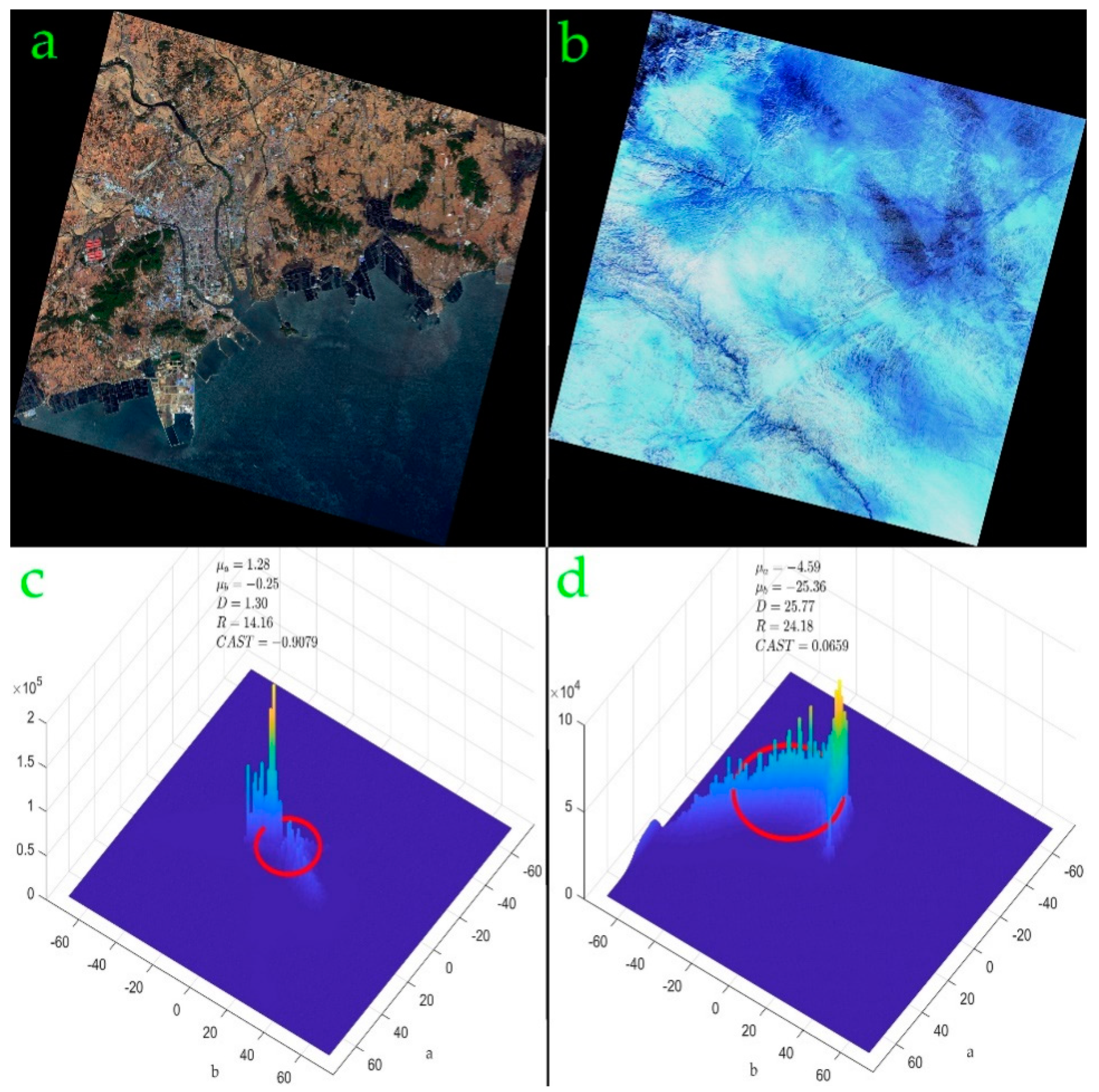
The color cast index CAST, mean value of component a μa, mean value of component b μb, the distance between the center of the equivalent circle and the neutral axis D and the radius of equivalent circle R were selected as our features to reflect the degree of color cast in an image (Figure 2). CAST, D, and R can be computed according to Equations (5)–(7):
CAST   =   ( D     R ) / R ,
D   =   μ a 2   +   μ b 2 ,
R   =   σ a 2   +   σ b 2 ,
in which σa and σb represent the standard deviation of component a and b, respectively.
Zhi [24] and Weihua [25] pointed that Near Neutral Objects (NNO) are important in color cast detection as the colorless surface in an image (the gray surface under standard white light, that is, the NNO of the color image) can fully reflect the color of the incident light. Therefore, as long as the gray surfaces in the scene are extracted, the deviation of image illumination can be estimated by the color deviation of the NNO area. The NNO area can be obtained as follows [25]:
If pixel I(i, j) belongs to NNO area, then it satisfies
{ 35     L i , j     95   a i , j 2   +   b i , j 2     d 4 ,   d = max   { a i , j 2   +   b i , j 2 } ( d   is   non isolated ) I ( i ,   j )   is   non isolated     ,
where L, a and b represent the corresponding components in CIELAB color space. Zhi [24] found that the changing rates of D and R (Dcr and Rcr) in both the whole image and NNO area are sensitive to color cast, thus were added into our features. They can be computed by Equations (9) and (10):
D cr = ( D     D NNO ) / D ,
R cr = ( R     R NNO ) / R .
Color Colorfulness Index (CCI) was found helpful for measurement of colorfulness. Hasler and Süsstrunk [26] proposed three estimations of CCI based on experiments, among which the third used a computationally efficient approach as described by Equations (11)–(15):
CCI   =   σ rgyb   +   0 . 3   ×   μ rgyb ,
σ rgyb   =   σ rg 2   +   σ yb 2 ,
μ rgyb   =   μ rg 2   +   μ yb 2 ,
rg = R − G,
yb = 1/2 (R + G) − B.
R, G, and B stand for the Red, Green, and Blue band of images, respectively. σ means standard deviation, μ average value, rg the difference between Red and Green, and yb the difference between Yellow and Blue. As shown in Table 1, abnormal images have usually brighter colors than normal ones, thus CCI for each image was computed and added into our features.
Finally, the “black edge” of satellite images caused by geotransform was found noteworthy. Images with abnormal shape or data missing may have different “black pixel ratio” compared to the normal ones. Besides, computation of features such as mean value of bands may be disturbed by 0 values in the “black edge”. A new feature NoneZeroRatio that means the ratio of pixels is not (0, 0, 0) was thus introduced to re-compute the above features by its mask. Naturally, the white pixels have the same problem, especially for images with abnormal color of cloud or snow. Again, a feature named “WhitePixelRatio” (The proportion of the number of pixels whose pixel values are greater than 253 in the total number of pixels in the three bands) was added. The mask of “NoneWhitePixel” was intersected with that of “NoneZeroPixel” to form our final mask, on which our above features are computed.

3.2. Model

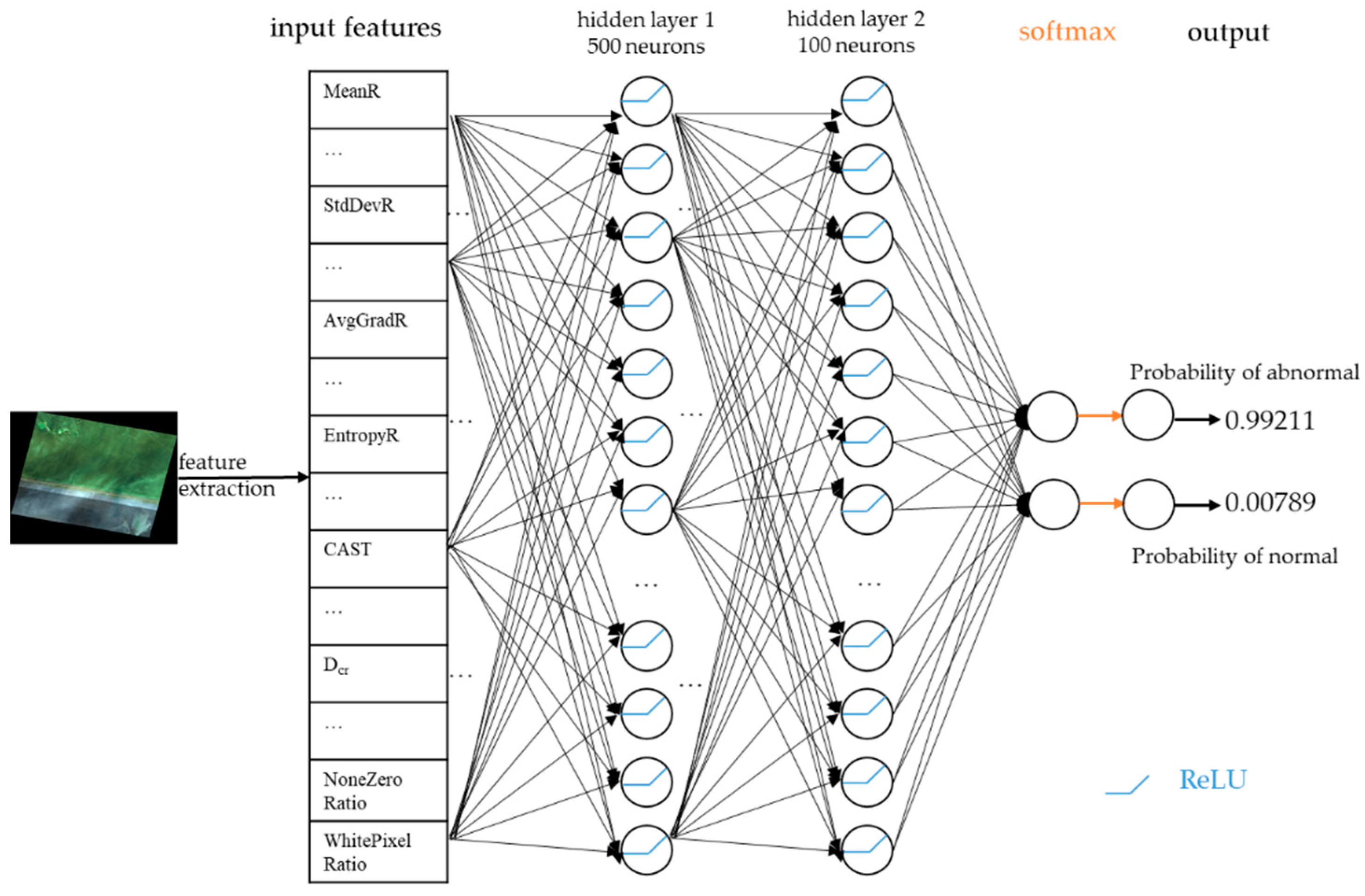
Based on a series of experiments (see Section 4.4), our ANN model was designed as follows. The model has two hidden layers, of which the first layer contains 500 neurons and the second 100. The activation function is ReLU. The architecture of our model is shown in Figure 3. It should be noted that before fed into the network, all the input features should first be normalized to a standard normal distribution, N (0, 1), to eliminate the scale differences between different features and facilitate training of ANN [27].

3.3. Interpretability

ANN is generally a black box as the inference result of the network is difficult to explain [27]. A multitude of research efforts have been directed towards the interpretability of ANN and deep learning. Marco et al. [28] proposed LIME, a novel explanation technique that explains the predictions of any classifier in an interpretable and faithful manner, by learning an interpretable model locally around the prediction. Montavon et al. [29] put forward a method called deep Taylor decomposition to efficiently utilize the structure of the network by back-propagating explanations from the output layer to the input layer. Selvaraju et al. [30] raised Grad-CAM to produce “visual explanations” of convolutional neural networks (CNNs).
A simple method based on local gradient approximation (LGA) is to be detailed below. The network can be regarded as a complex non-linear function F, and the feed forward progress can be described as Equation (16)
y   =   F ( x ) ,
where x stands for the vector of input features, and y the output. The gradient of ith dimension of x, xi, can be approximated as Equation (17).
F ( x ) x i F ( x + ε i ) F ( x ε i ) 2 ε ,
where εi is a vector in which ε (here ε is a sufficiently small value) is set as the value of the i-th element and 0 the value of all the other elements. All the features are normalized to N (0, 1) firstly. The absolute value of the gradient could be regarded as the importance of corresponding features. After computing out the importance factors for all the input features, we can have a general conclusion on the influence of different features, which is an efficient method for interpretability of our model.

4. Experiments and Results

This part first compares popular machine learning algorithms on our dataset to prove that ANN is the optimal algorithm to solve the proposed problem. Experiments were conducted to verify the effectiveness of our designed features and the performance of our model on different subclasses of abnormal images evaluated. Network architecture search (NAS) was adopted to identify the best network. Finally, examples of local gradient approximation would be presented to help explain the inference of our network.
Adam, an algorithm for first-order gradient-based optimization of stochastic objective functions was adopted to train our ANN model [31]. Its optimization process is somewhat random, leading to fluctuations in the results. To reduce the impact of fluctuations and make the results convincing, each test was repeated for 300 times to obtain the mean and standard deviation of F1 score and recall. To avoid overfitting, the model was trained for 100 epochs and the best F1 score and recall were recorded for calculation of the mean and standard deviation.

4.1. Comparison of ML Algorithms

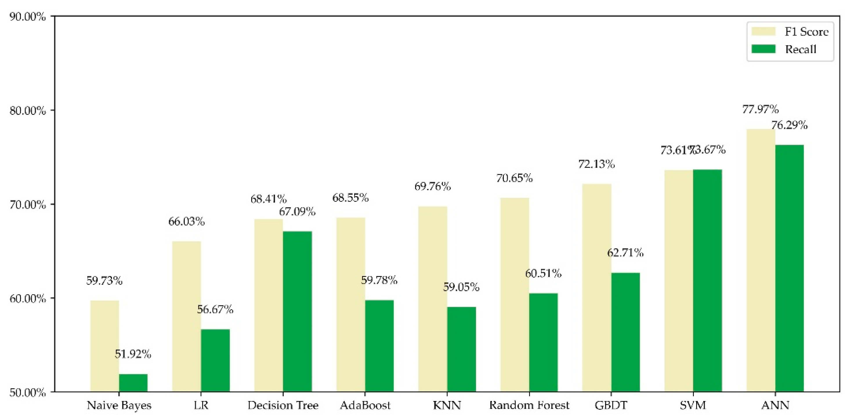
To prove that the ANN model is the best choice for our problem, we tested some popular ML algorithms on our dataset under the same input features mentioned in Section 3.1 for comparison. After being trained on the training set, the algorithms were validated on the validation set. The results are shown in Figure 4.
It can be observed that all the algorithms have a recall of over 50% and F1 score of over 60%, but details vary. Naïve Bayes performs worst while ANN performs best. Decision Tree records low F1 score but high recall, revealing its relatively low precision. SVM performs ordinarily but still not as good as ANN. The experiment results prove that ANN is the most suitable ML algorithm for our problem.

4.2. Growing and Ablation Study

This part explores the performance of our features by adding them to input group by group (namely, growing), and then removing them (namely, ablation), verifying the effectiveness of our designed features and the importance of each feature group. To save time, we used an ANN model having 2 hidden layers with both 50 neurons throughout this part.
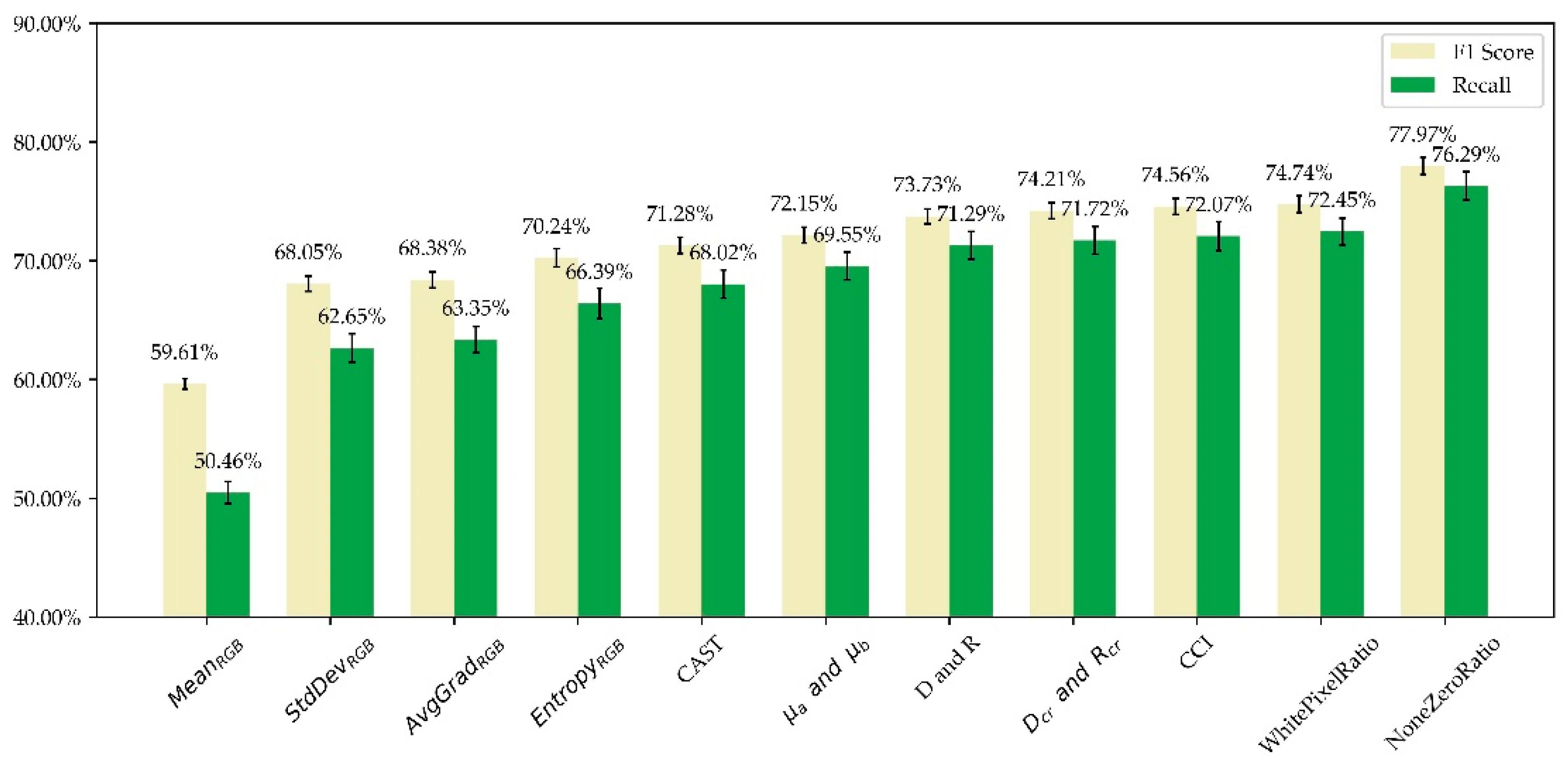
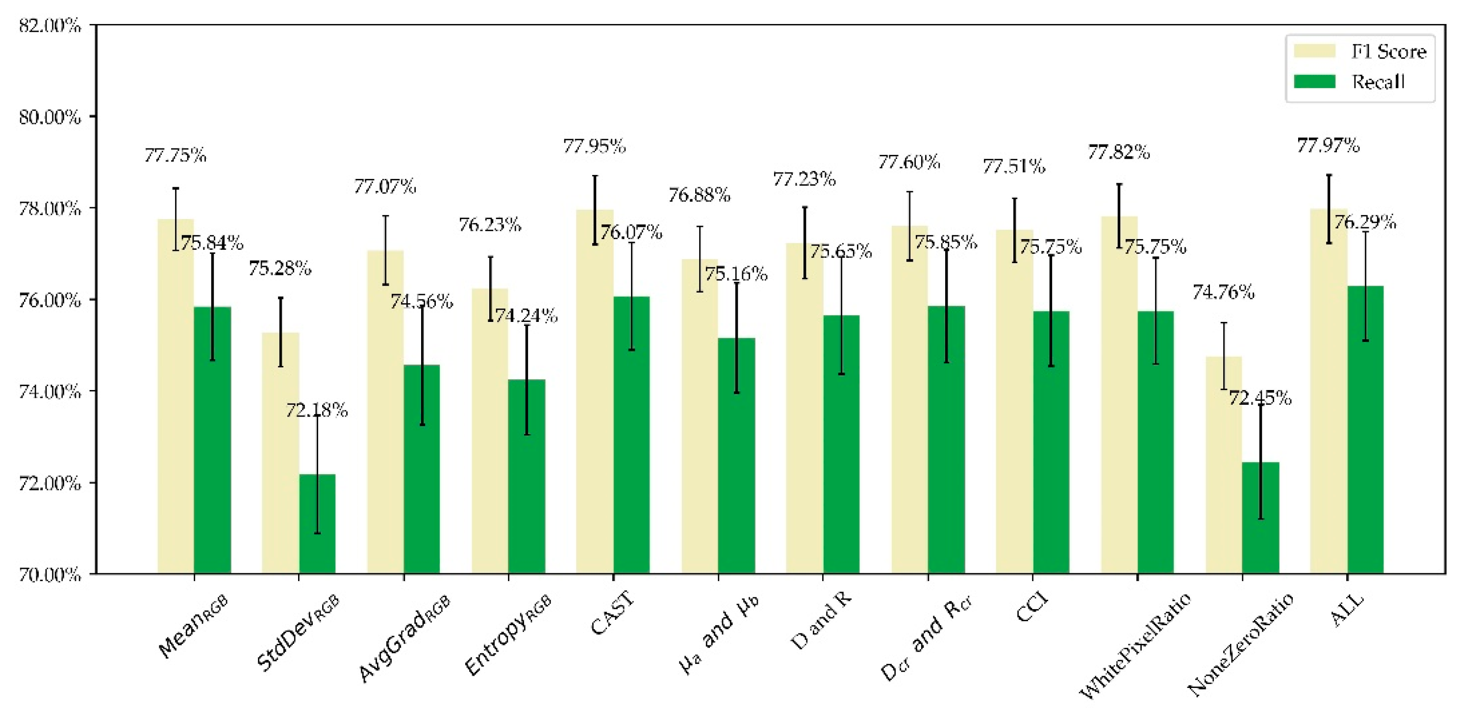
In the growing study, the features were added by the order of: MeanRGB, StdDevRGB, AvgGradRGB, EntropyRGB, CAST, μa and μb, D and R, Dcr and Rcr, CCI, NoneZeroRatio, WhitePixelRatio. The result is shown in Figure 5.
We can see that the mean values of F1 score and recall increase with the growing input features, verifying the effectiveness of our designed features. Specifically, F1 score rises dramatically when NoneZeroRatio is added, in part because images with data loss contain lots of zero pixels while the remaining areas look normal. It should be noted that under only three input features of MeanRGB, the model’s accuracy score reaches 81.42%, which is incredibly high. However, the model’s recall is only 50.46%, meaning the model could merely find half of the abnormal images. Hence, as we mentioned above, F1 score, the harmonic mean of precision and recall, should be prioritized, which has experienced a significant growth in Figure 5.
In the ablation experiment, the eleven groups of input features were removed one by one, and the remaining 10 groups of features were used to train the model. The results are shown in Figure 6.
After groups of input features were removed, F1 score and recall more or less fall down, demonstrating our designed features’ positive contributions to the model. MeanRGB, CAST and WhitePixelRatio seem to exert little influence on our model, while StdDevRGB and NoneZeroRatio have significant influence on the model. Many images have local anomalies and the mean value of all the pixels in an image remains steady, perhaps rendering the MeanRGB less discriminative. Nevertheless, the varying distribution of pixel values on normal and abnormal images makes StdDevRGB, AvgGradRGB and EntropyRGB outweigh other features to the model. StdDevRGB is more discriminative because it is more sensitive to extreme pixel values. CAST is a derived variable from D and R, which are more important than CAST in Figure 6. This is confusing and maybe derived features are sometimes unnecessary. NoneZeroRatio is important because images with data loss share lots of zero pixels as mentioned above; while WhitePixelRatio is less important perhaps because the number of white pixels is relatively small due to strict screening conditions. Although certain features bear little contribution to our model, they are reasonable and can help explain the inference of the model as shown in Section 4.5.

4.3. Performance on Different Subclasses

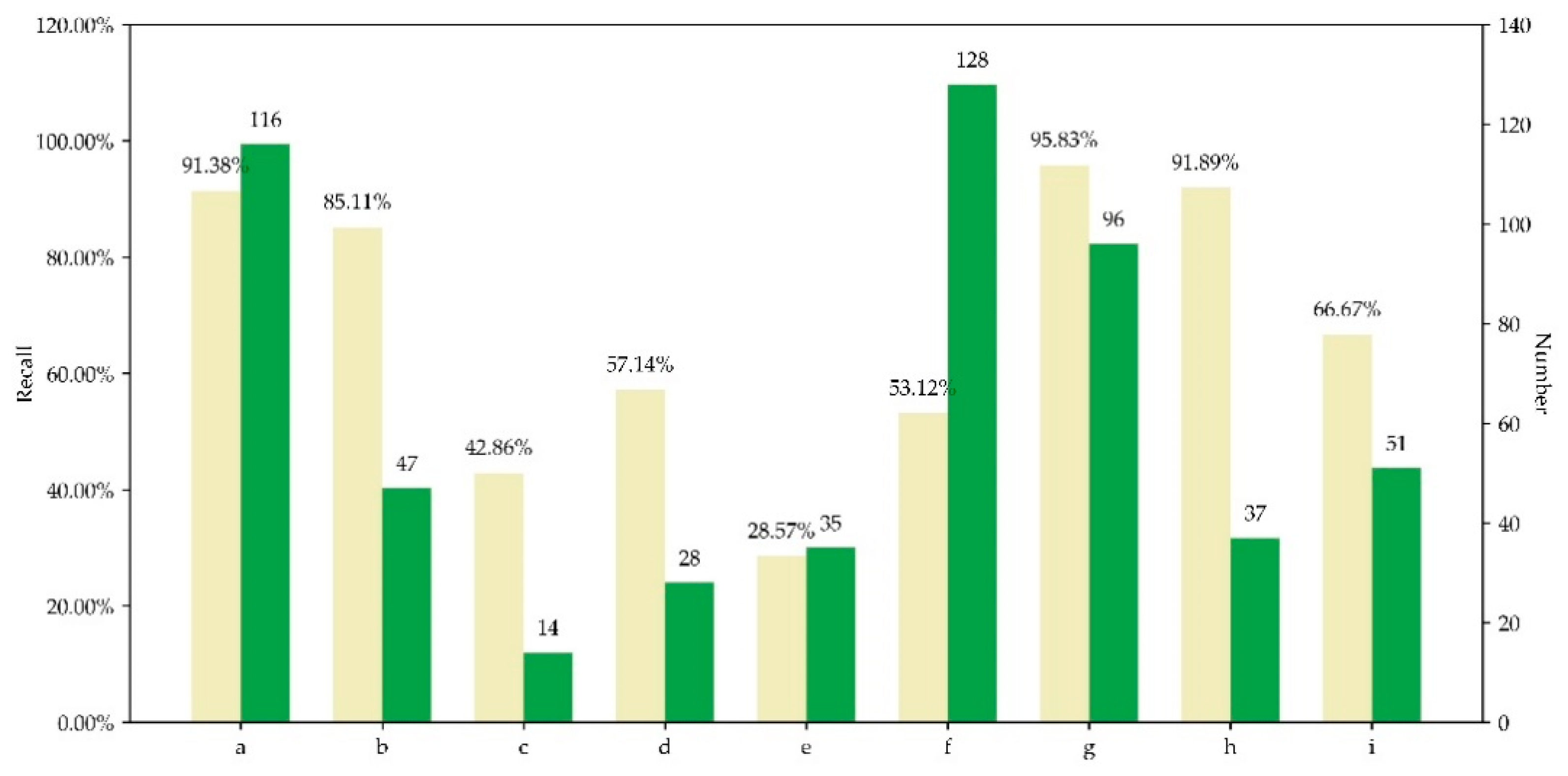
Our model aims to uniformly identify abnormal images with diversified anomalies, thus its performance on every subclass of anomaly is important. This study evaluated the recall of our model on each validation set of subclasses, and the results are shown in Figure 7. Again, the model with 2 hidden layers with both 50 neurons was used.
The model performed well on subclasses of a, b, g, h, and i, and not so good on c, d, e, and f. Due to lack of samples regarding subclasses of c, d, and e, the model’s correct inference about them was hindered. Subclass f contains images with abnormal color of cloud or snow. Though with enough samples, the model performed bad on subclass f probably in that the normal set also contains images with cloud or snow, whose mere difference with abnormal images lies in their pixels of abnormal colors. Probably overridden by highlighted pixels such as cloud or snow, those pixels contributed relatively less to the features, impeding the model’s identification. Nevertheless, all the above problems can be fixed in the future by continuous collection of samples and optimization of feature design. In general, the framework is able to identify different anomaly types uniformly.

4.4. Network Architecture Search

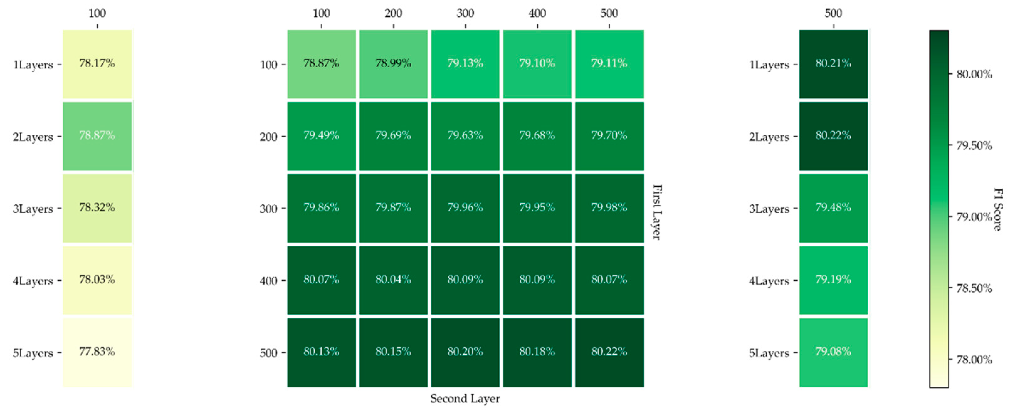
Based on reinforced learning, Network Architecture Search (NAS) is a hot field in deep learning [32,33]. Although our model tends to shallow learning, NAS was still adopted to identify the best structure of network. Our method prioritized two factors: number of hidden layers and neurons of each layer. Brute force search was conducted to obtain the best model. Similarly, tests for each model were repeated for 300 times and the mean value of best F1 score was recorded. The results can be seen in Figure 8.
We can see that the increase in the number of neurons in the first layer performs better than that in the second layer. Fewer neurons mean less information transformed and learned, and if the first layer outputs poor information, whatever the second layer is, the result would be unfavorable. As for the depth of network, to save time, only two groups of settings were tested, where the layers ranged from 1 to 5, and the neurons of 100 and 500. In theory, more layers entail better fitting ability and better performance. However, the results show that when the layers are more than 2, the network performs even worse. He et al. [34] pointed out that deeper network is not necessarily accompanied by better performance as deepened network is indeed a “degradation” that intensifies the difficulty of training. Finally, in consideration of accuracy and time, the first layer was set 500 neurons and the second 100 neurons.

4.5. Interpretability of the Model

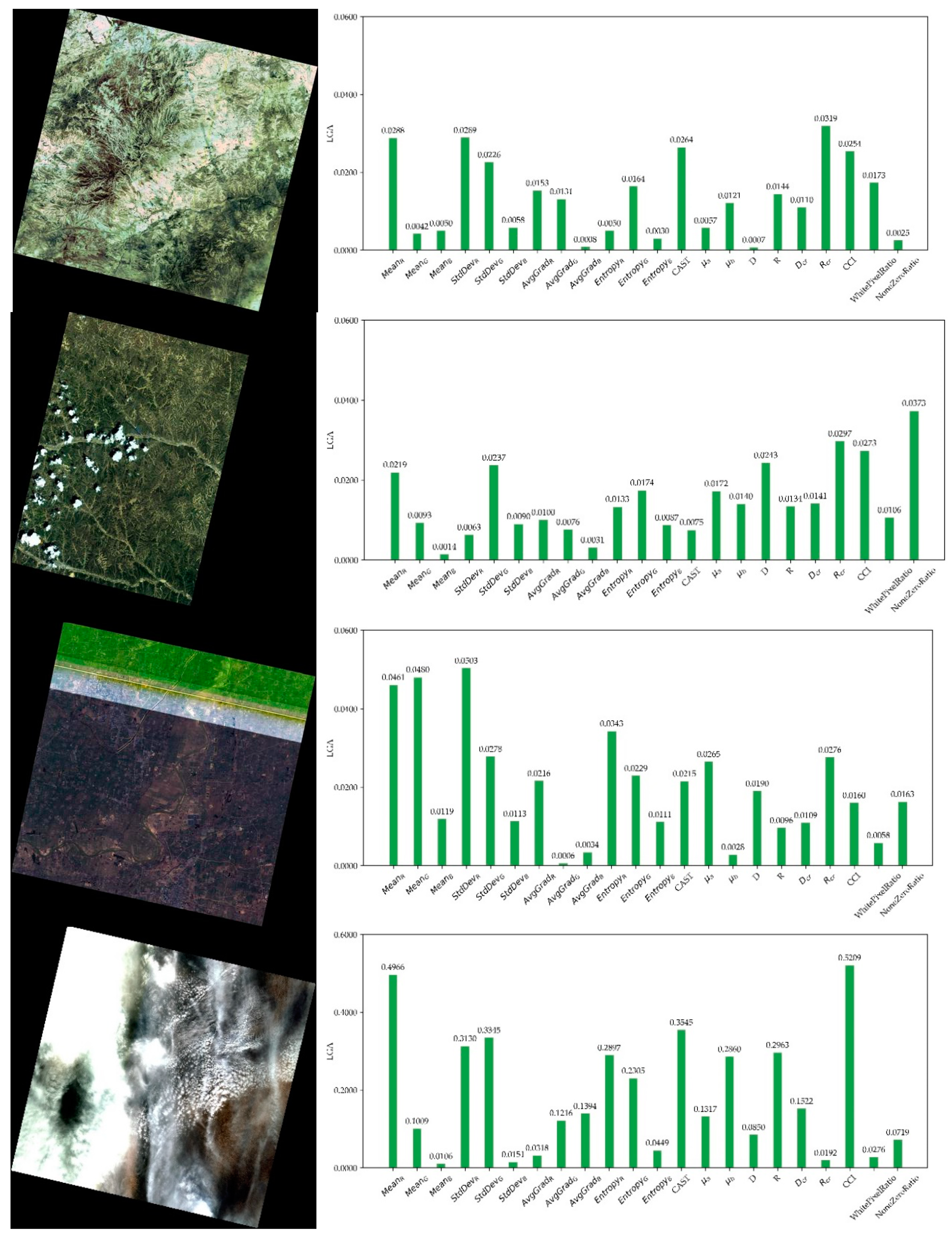
ε was set to be 0.001 and the method based on local gradient approximation was tested. Furthermore, the ANN model having 2 hidden layers with both 50 neurons was adopted. The examples are shown in Figure 9.
In Figure 9, all the four images are inferred as abnormal by our model. Figure 9a features obvious green color cast. Correspondingly, CAST and Rcr have relatively high LGA, indicating that color cast is a main reason for labeling of abnormal. Figure 9b shows an image with data loss on the right side. Logically, NoneZeroRatio comes as the most prominent feature in LGAs. Figure 9c is an image with abnormal horizontal stripe. In the LGAs, MeanG is reasonably high due to the green stripe. Figure 9d has abnormal color of cloud, for which CCI plays an important role. It should be noted that MeanR has usually high LGA, probably because red objects are rare in satellite images, making red features more sensitive. Generally, the method based on LGA is effective in interpreting the output of our ANN model.

5. Discussions

5.1. Innovations

The study’s innovation lies mainly in the design of a unified automatic framework for multi-type anomaly detection from massive raw satellite images based on ANN. Besides, our well-designed features closely related to data may provide useful reference for similar works. Saving costs and performing well, the proposed framework can be implemented easily and integrated seamlessly into the product line of satellite images.
The systematic experiments of both growing and ablation tests have strongly proved the effectiveness of our designed features. The model’s performance on each subclass of anomaly was tested and analyzed to prove the proposed model’s ability to identify different anomaly types uniformly. The network architecture search results were conducive to identification of the best network, and acquirement of knowledge about the influence of depth and width on ANN on our dataset. In the meantime, a simple method, i.e., local gradient approximation, was proposed to interpret the inference of ANN, which was proved effective by experiments.
Sometimes the proposed model shows low sensitivity to certain types of anomalies because of their few occurrence frequency and samples for training. To solve this problem, new samples could be continuously put into our dataset for updating, and new features extracted and added to the original features for retraining. Feature extraction and model retraining could be completed fast enough in our model to ensure rapid and smooth version updating, which is important in industrial production. Moreover, in the case that new anomaly type emerges in the future, our method could also be extended for adaptation. Again, new features that are sensitive to the new anomaly type should be designed and added to the original feature set for model retraining. In a word, our model is life-long, extensible, and flexible.

5.2. Weaknesses

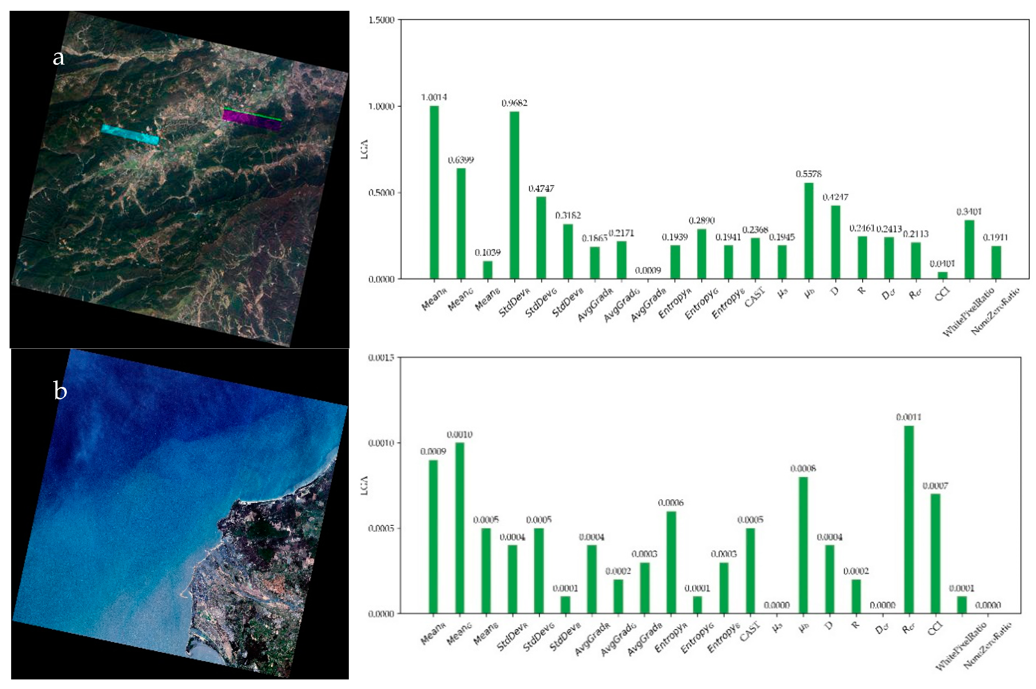
Although our method performs well, there are still some weaknesses. First, the proposed model is not sensitive enough to certain images with stripe-like anomaly or small rectangle colored block anomaly, which are normal generally but abnormal locally as shown in Figure 10a. Our designed features are all based on global statistics, which are position-independent, meaning that small local abnormal distribution of pixels may be overridden by global normal distribution. Second, some normal images, especially images of desert or seaside areas, may be reported falsely as can be seen in Figure 10b. This is probably caused by the simple tone of the whole image, such as the brown color in desert or the blue color of sea, leading to the model’s misjudgment of color cast. The weaknesses reveal that our framework still has room for improvement possibly by designing better features.
Figure 10 presents examples for incorrect detection and false alarm by our model. The two small colored rectangles in Figure 10a failed to attract the model’s attention and were falsely inferred as normal. Figure 10b shows a seaside image full of blue, yet the model mistakenly inferred it as color cast. In the LGA, Rcr, and μb show important influence, proving the above conjecture.

5.3. Future Work

In view of the weaknesses of our study, we intend to advance our future work by the following means.
First, more effective features are to be designed for better inference of anomalies. Position-dependent features are needed for identification of small local color anomalies. Block-wise statistics and even some line detection algorithms maybe inspirational, yet these methods are complicated and cannot adapt to all kinds of satellite images. For example, the size of block in block-wise statistics is hard to define, and some roads and huge buildings would be shown as straight lines, destroying line detection. This is also the reason why we did not add these features to our framework.
Second, instead of bi-classification, multi-classification may be realized as the anomalies themselves are various. The biggest obstacle now is the shortage of abnormal samples, which may greatly affect the model’s performance. Fortunately, more samples could be collected over time.
Then, instead of classification, the problem here can also be solved by means of regression. Specifically, the input images could be scored between 0 and 1, in which 0 entails normal and 1 abnormal. The starting point of this idea is that the degree of anomaly is so different among images that some are totally unusable while some are tolerable. The challenge is that the grading progress is subjective, to which a potential solution is multi-labeling and mean score, though it is labor consuming.
Finally, having made substantial breakthroughs in computer vision tasks such as sematic segmentation and object detection, CNN would also perform well on image classification, though the number of samples here might not be enough for deep training. Furthermore, the cost of time and computing resources like GPU could not be ignored, which is relatively small in our current light-weight ANN model.

6. Conclusions

This study proposes a unified automatic framework for detecting multi-type anomalies from massive raw satellite images based on ANN and well-designed representative features. The dataset was designed elaborately for even distribution of samples. A series of experiments have proved the effectiveness of our model and designed features. Network architecture search was adopted to find the good architecture of network. The model’s performance on subclasses of anomalies was tested to prove that our model can identify diversified anomalies uniformly. A simple but useful method was employed to explain the inference of ANN based on local gradient approximation. In general, being life-long, extensible, and flexible, the proposed framework can be seamlessly integrated into product lines. Though having some drawbacks, our framework takes the leading role in the field of automatic detection of abnormal images from massive raw satellite images, especially in remote sensing data center. This work will provide useful references for similar image-producing scenes where detection of abnormal images is needed.

Author Contributions

Conceptualization, H.W. and J.Y.; Funding acquisition, W.Y. and B.L.; Methodology, H.W. and J.Y.; Project administration, W.Y.; Resources, H.W. and W.Y.; Supervision, W.Y. and B.L.; Validation, R.M. and W.W.; Visualization, R.M. and J.Y.; Writing—original draft, J.Y.; Writing—review and editing, H.W., R.M. and W.W. All authors have read and agreed to the published version of the manuscript.

Funding

This research received no external funding.

Acknowledgments

The authors wish to thank the editors and reviewers.

Conflicts of Interest

The authors declare no conflict of interest.

References

  1. Zhang, B. Current Status and Future Prospects of Remote Sensing. Bull. Chin. Acad. Sci. 2017, 32, 774–784. [Google Scholar]
  2. Li, J.; Pei, Y.; Zhao, S.; Xiao, R.; Sang, X.; Zhang, C. A Review of Remote Sensing for Environmental Monitoring in China. Remote Sens. 2020, 12, 1130. [Google Scholar] [CrossRef] [Green Version]
  3. Gasparini, F.; Schettini, R. Color balancing of digital photos using simple image statistics. Pattern Recognit. 2004, 37, 1201–1217. [Google Scholar] [CrossRef]
  4. Jordan, M.I.; Mitchell, T.M. Machine Learning: Trends, Perspectives, and Prospects. Science 2015, 349, 255–260. [Google Scholar] [CrossRef] [PubMed]
  5. Mitchell, T.M. Introduction. In Machine Learning, 1st ed.; McGraw-Hill: New York, NY, USA, 1997. [Google Scholar]
  6. Christopher, M.B. Introduction. In Machine Learning and Pattern Recognition, 1st ed.; Springer: Berlin, Germany, 2006. [Google Scholar]
  7. Ian, G.; Yoshua, B.; Aaron, C. Machine Learning Basics. In Deep Learning, 1st ed.; MIT Press: Cambridge, MA, USA, 2016. [Google Scholar]
  8. Schmidhuber, J. Deep Learning in Neural Networks: An Overview. Neural Netw. 2015, 61, 85–117. [Google Scholar] [CrossRef] [PubMed] [Green Version]
  9. Nair, V.; Hinton, G. Rectified Linear Units Improve Restricted Boltzmann Machines. In Proceedings of the 27th International Conference on Machine Learning (ICML), Haifa, Israel, 21–24 June 2010. [Google Scholar]
  10. Ramachandran, P.; Zoph, B.; Le, Q.V. Searching for Activation Functions. In Proceedings of the International Conference on Learning Representations (ICLR), Vancouver, BC, Canada, 30 April–3 May 2018. [Google Scholar]
  11. Rumelhart, D.E.; Hinton, G.E.; Williams, R.J. Learning representations by back-propagating errors. Nature 1986, 323, 533–536. [Google Scholar] [CrossRef]
  12. Lecun, Y.; Bengio, Y.; Hinton, G. Deep Learning. Nature 2015, 521, 436–444. [Google Scholar] [CrossRef] [PubMed]
  13. Kaur, A.; Wasson, V. A Novel Approach to no-Reference Image Quality Assessment using Canny Magnitude Based upon Neural Network. In Proceedings of the 2nd IEEE International Conference on Recent Trends in Electronics, Information and Communication Technology (RTEICT), Bangalore, India, 19–20 May 2017. [Google Scholar]
  14. Zhai, G.; Min, X. Perceptual image quality assessment: A survey. Sci. China Inf. Sci. 2020, 63, 211301. [Google Scholar] [CrossRef]
  15. Alaql, O.; Ghazinour, K.; Chang, C. Classification of Image Distortions Based on Features Evaluation. In Proceedings of the 18th IEEE International Symposium on Multimedia (IEEE ISM), San Jose, CA, USA, 11–13 December 2016. [Google Scholar] [CrossRef]
  16. Wang, Z.; Athar, S.; Wang, Z. Blind Quality Assessment of Multiply Distorted Images Using Deep Neural Networks. In Proceedings of the International Conference on Image Analysis and Recognition (ICIAR), Waterloo, ON, Canada, 24–26 June 2019. [Google Scholar]
  17. Sebastian, B.; Dominique, M.; Thomas, W.; Wojciech, S. A deep neural network for image quality assessment. In Proceedings of the IEEE International Conference on Image Processing (ICIP), Phoenix, AZ, USA, 25–28 September 2016; pp. 3773–3777. [Google Scholar] [CrossRef]
  18. Xia, Y.; Chen, Z. Quality Assessment for Remote Sensing Images: Approaches and Applications. In Proceedings of the IEEE International Conference on Systems Man and Cybernetics Conference, City University of Hong Kong, Hong Kong, China, 9–12 October 2015. [Google Scholar] [CrossRef]
  19. Agudelo-Medina, O.A.; Benitez-Restrepo, H.D.; Vivone, G.; Bovik, A. Perceptual quality assessment of pan-sharpened images. Remote Sens. 2019, 11, 877. [Google Scholar] [CrossRef] [Green Version]
  20. Jingxiang, Y.; Yongqiang, Z.; Chen, Y.; Cheung-Wai, C.J. No-reference hyperspectral image quality assessment via quality-sensitive features learning. Remote Sens. 2017, 9, 305. [Google Scholar] [CrossRef] [Green Version]
  21. Javan, F.D.; Samadzadegan, F.; Reinartz, P. Spatial Quality Assessment of Pan-Sharpened High Resolution Satellite Imagery Based on an Automatically Estimated Edge Based Metric. Remote Sens. 2013, 5, 6539–6559. [Google Scholar] [CrossRef]
  22. Alice, Z.; Amanda, C. Introduction. In Feature Engineering for Machine Learning: Principles and Techniques for Data Scientists, 1st ed.; O’Reilly Media: Sebastopol, CA, USA, 2018. [Google Scholar]
  23. Hunt, R. Measuring Color, 3rd ed.; Fountain Press: Kampala, Uganda, 1998. [Google Scholar]
  24. Zhi, J. The Research of Color Cast Detection in Lab Color Space. Master’s Thesis, Xidian University, Xi’an, China, 2014. [Google Scholar]
  25. Weihua, X.; Brain, F.; Lilong, S. Automatic White Balancing via Grey Surface Identification. In Proceedings of the 15th Color Imaging Conference, Albuquerque, NM, USA, 5–9 November 2007. [Google Scholar]
  26. Hasler, D.; Süsstrunk, S. Measuring Colorfulness in Natural Images. In Human Vision and Electronic Imaging VIII; SPIE: Bellingham, WA, USA, 2003; Volume 5007. [Google Scholar]
  27. Zhou, Z.H. Neural Networks. In Machine Learning, 1st ed.; Tsinghua University Press: Beijing, China, 2016. [Google Scholar]
  28. Marco, T.R.; Sameer, S.; Carlos, G. Why Should I Trust You?: Explaining the Predictions of Any Classifier. In Proceedings of the 22nd ACM SIGKDD International Conference on Knowledge Discovery and Data Mining (KDD), San Francisco, CA, USA, 13–17 August 2016. [Google Scholar] [CrossRef]
  29. Montavon, G.; Lapuschkin, S.; Binder, A.; Samek, W.K.R. Explaining nonlinear classification decisions with deep Taylor decomposition. Pattern Recognit. 2017, 65, 211–222. [Google Scholar] [CrossRef]
  30. Selvaraju, R.R.; Cogswell, M.; Das, A.; Vedantam, R.; Parikh, D.; Batra, D. Grad-CAM: Visual Explanations from Deep Networks via Gradient-Based Localization. Int. J. Comput. Vis. 2020, 128, 336–359. [Google Scholar] [CrossRef] [Green Version]
  31. Kingma, D.P.; Ba, J. Adam: A Method for Stochastic Optimization. In Proceedings of the International Conference on Learning Representations, San Diego, CA, USA, 7–9 May 2015. [Google Scholar]
  32. Baker, B.; Gupta, O.; Naik, N.; Raskar, R. Designing Neural Network Architectures using Reinforcement Learning. In Proceedings of the International Conference on Learning Representations (ICLR), Toulon, France, 24–26 April 2017. [Google Scholar]
  33. Bello, I.; Zoph, B.; Vasudevan, V.; Le, Q. Neural Optimizer Search with Reinforcement Learning. In Proceedings of the International Conference on Learning Representations (ICLR), Toulon, France, 24–26 April 2017. [Google Scholar]
  34. He, K.; Zhang, X.; Ren, S.; Sun, J. Deep Residual Learning for Image Recognition. In Proceedings of the IEEE Conference on Computer Vision and Pattern Recognition, Seattle, WA, USA, 27–30 June 2016; pp. 770–778. [Google Scholar] [CrossRef] [Green Version]
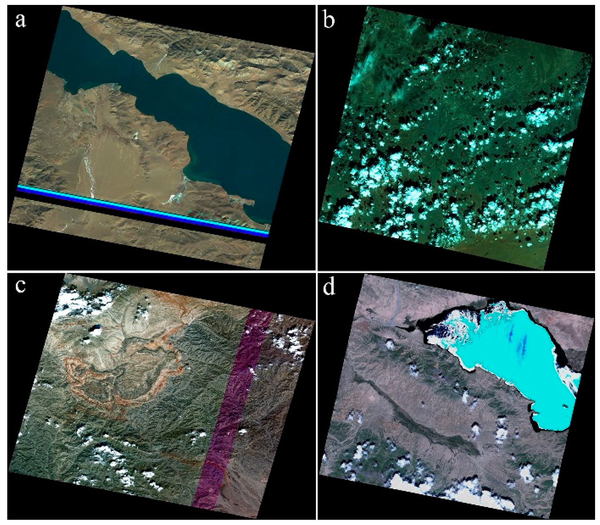
Figure 1. Examples of abnormal satellite images: (a) narrow-stripe data missing, (b) green color cast, (c) stripe with abnormal color, (d) pixels with extreme color. Best viewed in color.
Remotesensing 13 01506 g001
Figure 2. The 2D histogram of ab plane in CIELAB color space (a) a satellite image with normal color, (b) a satellite image with color cast, (c) 2D histogram of image a, (d) 2D histogram of image b. The red circles in (c, d) are the equivalent circles mentioned above. Compared with color cast images, normal images have smaller equivalent circles that are closer to the neutral axis. The CAST of normal images is close to −1, while that of color cast ones is usually greater than 0 and close to 1. Best viewed in color.
Remotesensing 13 01506 g002
Figure 3. Architecture of our ANN model.
Remotesensing 13 01506 g003
Figure 4. F1 score and recall of different machine learning algorithms on our dataset. ANN performs best among the classical algorithms. Note that the results were obtained through 300 repeated tests and the mean value was employed. The result of ANN was acquired through the architecture of two hidden layers with both 50 neurons.
Remotesensing 13 01506 g004
Figure 5. Results of growing study. Features were added to the input group by group. The results are the mean values obtained through 300 times of tests, and the black vertical disconnections indicate ± standard deviation. F1 score and recall “increase” with the growing features, indicating the effectiveness of our designed features.
Remotesensing 13 01506 g005
Figure 6. Results of ablation study. Features were removed groups by groups. The results are the mean values obtained through 300 times of tests, and the black vertical disconnections indicate ± standard deviation. The results of all the features are plotted on the right. F1 score and recall fall down more or less when any group of features is removed.
Remotesensing 13 01506 g006
Figure 7. The model’s performance on different subclasses. Both recall and sample number of verification set for each subclass are given. The code a–i is consistent with that in Table 1.
Remotesensing 13 01506 g007
Figure 8. Results of network architecture search. Best viewed in color. The green map represents different F1 scores. The 5 × 5 grids in the middle show the F1 scores of models with two hidden layers, while the vertical and horizontal axis stands respectively for the number of neurons of the first and second layer. The 5 × 1 grids on the left side show the F1 scores of models with 1 to 5 hidden layers that have 100 neurons per layer, and the 5 × 1 grids on the right side show the F1 scores of models with 1 to 5 hidden layers that have 500 neurons per layer.
Remotesensing 13 01506 g008
Figure 9. Results of LGA. Best viewed in color. Four satellite images on the left and LGA results on the right. All the four images are labeled abnormal by the model.
Remotesensing 13 01506 g009
Figure 10. Examples of incorrect detection and false alarm. Best viewed in color. (a) is a satellite image with an abnormal colored rectangle block, but the model inferred it as normal image. (b) shows a satellite image of seaside with normal color, but the model inferred it as abnormal image. LGA is shown on the right.
Remotesensing 13 01506 g010
Table 1. Numbers and examples of samples in the dataset.
CategorySubclassCodeSamples for TrainSamples for ValidationExample
Abnormaloverall extreme colora268116 Remotesensing 13 01506 i001
abnormal shape (including blocked data loss)b10747 Remotesensing 13 01506 i002
Remotesensing 13 01506 i003
abnormal colored rectangle blockc3114 Remotesensing 13 01506 i004
abnormal horizontal stripe (including horizontal narrow data loss)d6228 Remotesensing 13 01506 i005
Remotesensing 13 01506 i006
abnormal vertical stripee7935 Remotesensing 13 01506 i007
abnormal color of cloud or snowf296128 Remotesensing 13 01506 i008
blue color castg22296 Remotesensing 13 01506 i009
purple color casth8437 Remotesensing 13 01506 i010
other color casti11751 Remotesensing 13 01506 i011
Normal 32781405 Remotesensing 13 01506 i012
Publisher’s Note: MDPI stays neutral with regard to jurisdictional claims in published maps and institutional affiliations.