Article

Polar Stratospheric Clouds Detection at Belgrano II Antarctic Station with Visible Ground-Based Spectroscopic Measurements

1
Atmospheric Research and Instrumentation Branch, Instituto Nacional de Técnica Aeroespacial—INTA, Carretera de Ajalvir km4, 28850 Torrejón de Ardoz, Spain
2
National Antarctic Direction (DNA)/Argentinian Antarctic Institute (IAA), 25 de Mayo 1143, San Martín, Buenos Aires B1650HMK, Argentina
*
Author to whom correspondence should be addressed.
Remote Sens. 2021, 13(8), 1412; https://doi.org/10.3390/rs13081412
Submission received: 25 February 2021 / Revised: 26 March 2021 / Accepted: 2 April 2021 / Published: 7 April 2021
(This article belongs to the Special Issue Active and Passive Remote Sensing of Aerosols and Clouds)

Abstract

:
By studying the evolution of the color index (CI) during twilight at high latitudes, polar stratospheric clouds (PSCs) can be detected and characterized. In this work, this method has been applied to the measurements obtained by a visible ground-based spectrometer and PSCs have been studied over the Belgrano II Antarctic station for years 2018 and 2019. The methodology applied has been validated by full spherical radiative transfer simulations, which confirm that PSCs can be detected and their altitude estimated with this instrumentation. Moreover, our investigation shows that this method is useful even in presence of optically thin tropospheric clouds or aerosols. PSCs observed in this work have been classified by altitude. Our results are in good agreement with the stratospheric temperature evolution obtained by the global meteorological model ECMWF (European Centre for Medium Range Weather Forecasts) and with satellite PSCs observations from CALIPSO (Cloud-Aerosol-Lidar and Infrared Pathfinder Satellite Observations). To investigate the presence and long-term evolution of PSCs, the methodology used in this work could also be applied to foreseen and/or historical observations obtained with ground-based spectrometers such e. g. those dedicated to Differential Optical Absorption Spectroscopy (DOAS) for trace gas observation in Arctic and Antarctic sites.

Graphical Abstract

1. Introduction

Polar Stratospheric Clouds (PSCs) are often observed in the Arctic and Antarctic skies mostly during winter and spring. The formation of these clouds, composed by super-cooled ternary solutions (STS), nitric acid trihydrate (NAT), and/or ice particles [1], is mainly driven by temperature [2]. Some PSCs have been observed at temperatures up to 208 K. However most of the PSCs are formed at temperatures below 195 K, with a maximum close to the ice frost point (~188 K) [3]. These low temperatures are found in winter at stratospheric altitudes (12–30 km) inside a cold and stable polar vortex [1,4].
PSCs have been detected and studied using different sort of instruments. Detailed PSC characterization has been performed using in situ balloons and aircraft-borne instrumentation [5,6,7]. However, the temporal and spatial coverage of these observations is very limited. In addition, these campaigns are very scarce and complex, mainly in Antarctica. PSCs detection and characterization have also been investigated remotely using visible/near-infrared (NIR) scattered radiation [8], UV/visible star occultation [9] or infrared (IR) limb emission by different space and balloon-borne instruments [10,11,12,13,14,15,16]. From 2006, the Cloud-Aerosol Lidar with Orthogonal Polarization (CALIOP) [17] onboard the Cloud-Aerosol-Lidar and Infrared Pathfinder Satellite Observations (CALIPSO) is operating with high vertical, horizontal, and temporal resolution [3], and thus motivating numerous studies focused on the PSCs characterization [3,4,18,19,20,21]. Regarding ground-based remote sensing studies of PSCs, on Antarctica a few stations perform long-term PSCs observations, most of them using lidar instrumentation: Admunsen-Scott [22], McMurdo [4,23,24,25,26], Belgrano II [27], and Dumont d’Urville stations [28,29,30]. Lidars are able to provide data continuously during day and night, but they are complex (acquisition and maintenance) and low and thick tropospheric clouds, frequently observed at Antarctic stations, can mask the possible PSC observation [31]. As for ground-based studies of PSCs, Sarkissian et al. [32] proposed the use of the color index (CI), defined as the ratio between intensities at two different wavelengths, to detect PSCs at twilight (solar zenith angles (SZA) ~86° to 96°) using spectra recorded by a ground based UV–VIS spectrometer. The method proposed by Sarkissian and co-workers is based on the sunlight reddened due to Rayleigh opacity through long optical paths during twilight and the different wavelength dependence of the scattering cross-sections of particles (Mie theory [33]) and molecules (Rayleigh theory [34]). At high SZAs, the spectra provide information from the low stratosphere where PSCs are usually observed. In that work, the CI at a given SZA, CIsza, was defined as the ratio between the intensity at zenith at 550 and 350 nm. Using a pseudo-spherical single scattering radiative transfer model (RTM), they simulated different PSC scenarios based in four parameters: cloud altitude, geometrical and optical thickness, and scattering wavelength (λ) dependence (considering this dependence through a parameter: λ; with 0 < α < 3). The CI evolution at twilight in the presence of PSCs clearly differs from the Rayleigh atmosphere. Depending on the PSC type and the 4 considered parameters, the CI experiments a reddening or bluing towards higher SZAs. Tropospheric clouds and aerosols also influence the CI evolution. Trying to minimize this tropospheric contribution, in the work of Sarkissian et al. [32], the CIsza was normalized at its value at SZA = 90° (i.e., CInorm = CIsza/CI90). Following the same principle, similar methods have been applied to the detection of PSCs from ground-based spectroscopic observations in different works [35,36,37], all of them performed at Arctic latitudes and using simple single scattering models. However, the single scattering approximation is not suitable in this case as higher orders of scattering are expected within the cloud, as well as along the sun line of sight. Moreover, an accurate definition of the radiative processes present at high latitudes and high SZA requires full spherical RTM.
In this work, we present a method similar to Sarkissian’s based in the CI evolution at twilight obtained from a visible ground-based spectrometer deployed at the Antarctic Belgrano II station. The method here presented is supported by a multiple-scattering Monte-Carlo RTM [38] in spherical geometry, already employed for the detection and characterization of cirrus and water ice clouds on Mars [39,40,41]. In Section 2.1, the employed instrument and measurement site are described. Section 2.2 presents the ancillary data used to cross-check the validity of our results. A description of the PSC detection method is given in Section 2.3. Section 2.4 describes the RTM simulations of the CI signals under different scenarios. The method was then applied to the observations acquired during 2018 and 2019 PSCs season, and results were cross-checked with available CALIPSO data. The presentation and corresponding discussion of these data are included in Section 3. The main conclusions of this study will be established in Section 4.

2. Materials and Methods

2.1. Measurements

Spectra used in this work were recorded by a twin (UV/Vis) Multi-Axis Differential Optical Absorption Spectroscopy (MAX-DOAS, [42]) instrument located at Belgrano II station (77°52′S, 34°37′W; 256 m a.s.l., see Figure 1). The instrument, called NEVA-II, counts with an outdoor unit that scans the sky from the horizon to the zenith. The pointing system, with two coupled telescopes with a field of view of 1° each, collects the scattered sunlight and directs it into the indoor unit through two fiber bundles. The thermally stabilized indoor detection unit consists of two spectrometers, one operating in the Vis channel (415 to 542 nm) and the other in the UV spectral range (320–415 nm). Each spectrometer consists of a TRIAX 180 monochromator and a HAMAMATSU S7031-1008 Charge-Coupled Device (CCD) detector and has a spectral resolution of 0.5 nm. Data discussed in this work correspond to observations performed with the Vis channel. Observations with the UV spectrometer will also be addressed but only as a UV–VIS crosscheck exercise (see Section 3.2).
The whole instrument NEVA II, including the detector read-out electronics, was fully developed by INTA (Spanish National Institute for Aerospace Technology). It was designed for continuous operation under polar conditions and it is part of the NDACC (Network for the Detection of Atmospheric Composition Change, http://www.ndacc.org, accessed on 25 February 2021) since 2016. Thanks to a collaboration between the National Antarctic Direction of Argentina/Argentinian Antarctic Institute (DNA/IAA) and INTA, this instrument has been operating at the Antarctic research base of Belgrano II since 2011. It has been continuously probing the Antarctic stratosphere and troposphere to investigate, through the DOAS technique [43], trace gases such NO2, O3, OClO, and BrO (e.g., [44,45]). Note that the site of Belgrano II, located at the south coast of the Weddell Sea and the north of the Filchner Ice Helf (see Figure 1) remains well inside the polar vortex during wintertime [46] (see Figure 1) and thus it is characterized by the frequent presence of PSCs [47,48].
The spectral calibration of NEVA-II instrument, very stable over the years, is performed with a mercury/cadmium lamp at least twice per year. The temperature of the CCD and the monochromator is kept to −40 °C ± 0.05 °C, and all spectra are corrected by offset and dark current. The automatic measuring routine of the NEVA-II has two modes depending on the SZA: off-axis mode (i.e., vertical scan of atmosphere as long as SZA < 86°) and zenith mode (telescope fixed at zenith geometry for SZA 86–96°). Note that, since the method relies on scattered sunlight, no measurements are performed during the polar night (May–mid August). At twilight, the acquisition time of spectra can last from several seconds (SZA ~86°) up to 6 minutes for the highest SZAs, thus capturing the fast changes in sky brightness at this period. In this work, only spectra acquired at zenith mode are used for the detection and characterization of PSCs at twilight. This configuration allows us to probe the stratospheric layers where PSCs usually form.

2.2. Ancillary Data

2.2.1. Temperature profiles from the global meteorological model ECMWF (European Centre for Medium Range Weather Forecasts)

Since, as mentioned above, PSCs are very dependent on atmospheric temperature, the feasibility of the presence of PSCs over Belgrano II during our measurements was investigated using the vertical profiles of the atmospheric temperature above the research site obtained with the ERA5 data reanalysis from the global meteorological model ECMWF (European Centre for Medium Range Weather Forecasts) [49]. ERA5 was produced using 4D-Var data assimilation in CY41R2 of ECMWF’s Integrated Forecast System (IFS), with 137 model levels in the vertical. The ERA5 dataset contains one high resolution realization (HRES) with a resolution of 0.25 degrees and hourly outputs. The mentioned temperatures profiles were obtained in 2018 and 2019 using 119 model levels from surface up to ~40 km and twice a day (00:00 and 12:00 UTC). In addition, the horizontal temperature distribution shown in the Figure 1 was created using ERA5 data at 475 K isentropic level.

2.2.2. CALIPSO Data

The detection and altitude estimation of the PSC observed in this work were also cross-checked with CALIOP observations. The satellite data used for this exercise are the Lidar Level 2 operational PSC mask product (L2PSCMask, doi: 10.5067/CALIOP/CALIPSO/CAL_LID_L2_PSCMask-Prov-V1-00_L2-001.00). This product enables not only the detection of PSCs on the CALIPSO orbit track at 5 × 5 km (horizontal) and 0.18 km (vertical) resolution, but also the PSC classification based on their composition. Following the work of Pitts et al. [19,20], the CALIOP-PSCs are classified in six types depending on their composition: supercooled ternary solutions (STS), STS mixed with low, medium and high number density of nitric acid trihydrate (NAT) particles (STS + lowNAT, STS + medNAT, STS + highNAT, respectively), water ice PSCs and PSCs due to gravitational waves (WaveIce).

2.3. PSC Detection Method

As indicated in Section 1, the detection and characterization of PSCs is possible by observing the evolution of the CI with SZA at twilight (SZA between 90° and 95°) [32,35,36,37]. For a given SZA, the CI is defined as:
C I ( S Z A ) = I ( λ 1 , SZA ) I ( λ 2 , SZA )   ,
where I is the measured intensity at wavelengths λ1 and λ2. Taking into account the spectral range of our instrument, we selected λ1 = 520 nm (green) and λ2 = 420 nm (blue) to maximize the PSC signatures on the color index signals, and to avoid strong gas absorptions or Ring structures [50]. These wavelengths have been averaged over an interval of 0.5 nm to reduce noise. To facilitate the PSC detection, CI signals were normalized to the CI measured during a Rayleigh day, CIref:
C I n o r m ( S Z A ) = C I ( SZA ) C I r e f ( SZA )   ,
Throughout twilight, PSCs are evidenced as a maximum in the CInorm signal, and the SZA of this maximum depends on the cloud altitude. Due to the Rayleigh scattering, the shorter is the wavelength of the light, the higher is the probability of scattering along the line of sight (Rayleigh theory [34]). This effect results in the reddening of the atmosphere, and it is appreciable for large optical paths as those followed by sunlight during twilights. When PSCs are present during twilight, they produce a significant increase in the number of scatters at an altitude where there are also a large number of photons available, compare to lower altitudes. Thus, most of the scattering will occur there. This means that, in the presence of a PSC, we will observe a maximum in the CI, which value will increase with the altitude of the cloud.
Indeed, the shape of the CI evolution and the SZA of highest CI depend on different PSC properties such as the opacity or altitude. The method presented in this work is sensible to the altitude of the PSCs. In the following section, the influence of the PSC altitude, opacity, and phase function will be studied using a multiple scattering spherical Radiative Transfer Model (RTM). Additionally, with that RTM we will also investigate the influence of tropospheric clouds, of aerosols and of absorption on the CI evolution.

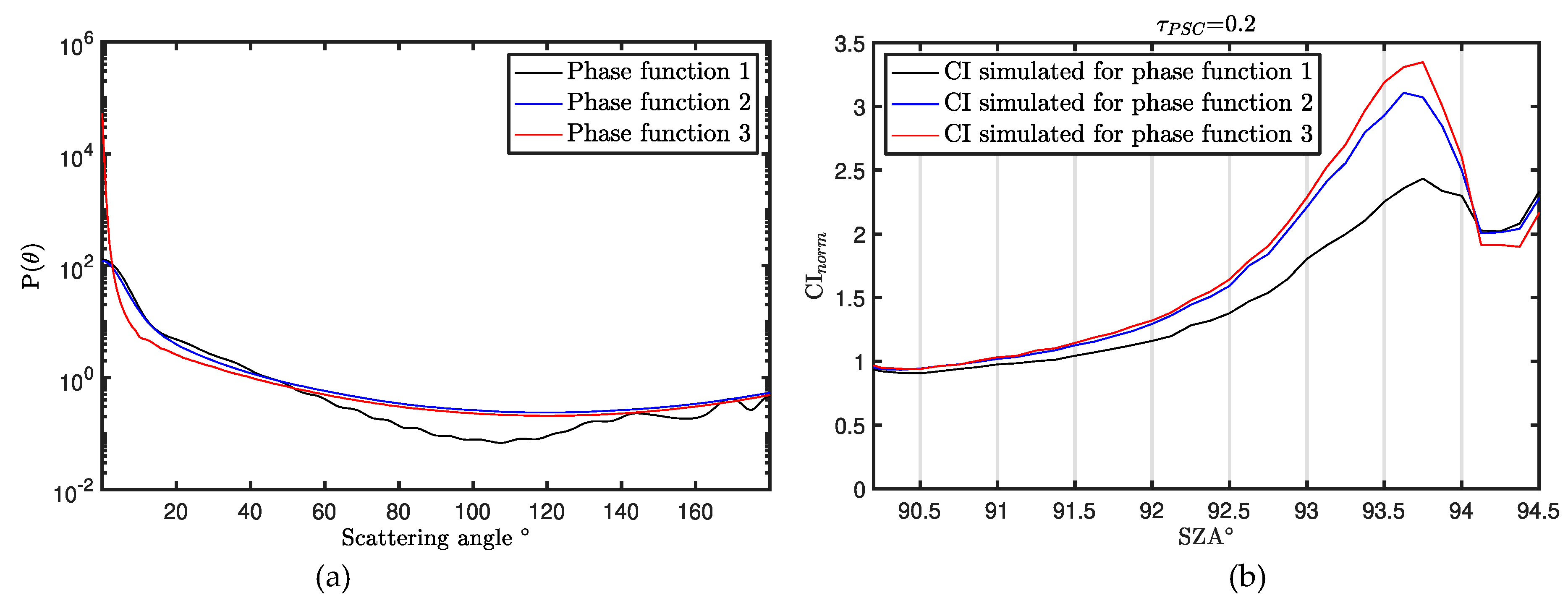
2.4. Model Simulations

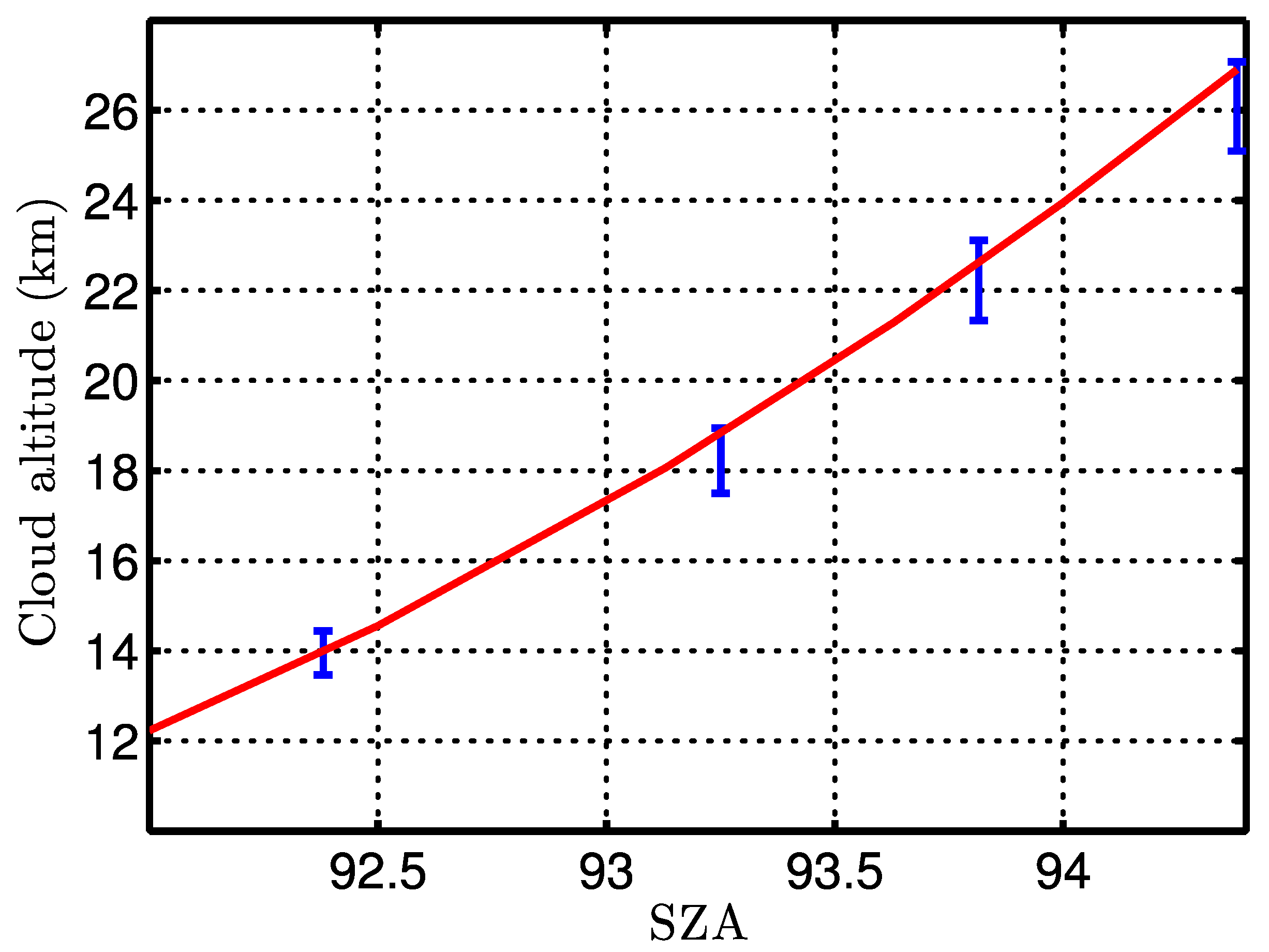
2.4.1. Retrieval Procedure

As explained in Section 2.2, the presence of high clouds (such PSCs) produces a maximum in the CI signal. Therefore, our first goal here is to simulate the CI signals in the presence of PSCs in order to evaluate which properties could be derived with ground-based remote sensing observations. The simulations of CI at twilight require a multiple scattering radiative-transfer code in spherical geometry. In this sense, this is a key difference between this work and those that made used of the single scattering approximation [32,35,36,37]. Here, we use a Monte-Carlo radiative model [38], previously employed for the detection and characterization of cirrus clouds [39] and water ice clouds on Mars [40,41]. A representative model for PSC-type cloud is a thin layer at a given altitude with a spatial distribution of cloud-particle density characterized by a Gaussian height profile, which is scaled to produce the required cloud optical depth. The scattering properties of cloud particles are described by the single scattering albedo ω and phase function P(θ). While the single scattering albedo at visible wavelengths is set to unity, the calculation of the phase function represents a major challenge. Indeed, the phase function depends, among other parameters, on the size and shape of cloud particles. As these parameters are highly variable for PSC-type clouds, a number of simulations were performed to evaluate the impact that these parameters may have on our analysis.
Figure 2 shows, as example, the evolution of different CI signals simulated by the Monte-Carlo RTM for different cloud altitudes (a) and optical depths (b). For these simulations, the aerosol optical depth was set to zero, and Rayleigh opacity was computed from standard profiles of pressure and temperature [51]. These simulations indicate that the SZA of highest CI, SZAmax, depends on the PSC’s altitude. Thus, for a given PSC detection case, the altitude of the cloud can be estimated by comparing the SZAmax with the values obtained by the simulations. Although Figure 2b indicates that the shape of the CI maximum depends on τPSC, our simulations show that this shape depends also on a number of different model parameters, such as the cloud particles radius, whose values are not well constrained. Figure 3 shows phase functions computed using T-Matrix for different effective radius reff (ranging from 1 to 10 µm) and particle shapes (a), along with CI signals simulated for these different phase functions (b). The rest of model parameters were set to hPSC = 22 km and τPSC = 0.2. These simulations indicate that, although the shape of the CI maximum depends on the cloud phase function, the SZA of highest CI does not significantly change with this parameter. Similar results were obtained for the geometrical thickness of the cloud or its optical depth. Therefore, we conclude that consistent PSC altitudes can be estimated by comparing the measured CI signals with the computed curves that relate the SZAmax and the cloud altitude (referred as hPSC-SZA curve hereafter).

2.4.2. Gas Absorption

For the simulations shown in the previous section, we did not include the effect of gas absorption. Although the wavelengths used to compute CI were selected to minimize this factor, we must evaluate the impact of gas absorption on the CI simulations. For the selected wavelengths (420 and 520 nm), gases that may impact CI signals are mainly NO2 and O3. Figure 4 illustrates NO2 and O3 density profiles characteristic of polar latitudes and for the months of August, September, and October (i.e., PSC season in the southern hemisphere). Ozone profiles correspond to monthly average values obtained from ozone soundings performed at Belgrano II from 1999 to 2006 [48]. NO2 profiles were obtained from standard atmosphere scaled to typical total column values of NO2 observed at the stations during the considered months [44]. From these profiles and the absorption cross-sections [52,53], the scattering and absorption coefficients of these gases were computed. Figure 5 shows the variation of the SZAmax with the PSC altitude (hPSC-SZA curve) for a cloud opacity τPSC = 0.2 and using the gas profiles given in Figure 4. Similar hPSC-SZA curves were computed for different values of τPSC and analogous results were obtained. Thus, for a given PSC detection case in the CI signal, the cloud altitude can be estimated by comparing the SZAmax with the values given in Figure 5, corresponding to a second order polynomial fitting of the simulations.

2.4.3. Low Tropospheric Clouds

For the simulations shown in Figure 5, we assumed that no low-altitude tropospheric clouds were present at twilight. However, given the extreme meteorology of the polar regions, PSC may be present under these conditions. Therefore, the impact of these low clouds on modelled CI signals must be examined. Note that, due to their low altitude, these lower clouds do not receive direct light for SZA > 90°. Therefore, they only affect the light scattered by the PSCs at higher altitudes. If the tropospheric cloud is very thick (i.e., opacities higher than 2), the PSC signature over the CI signal can be masked by the dispersion of the tropospheric cloud particles. However, if the tropospheric clouds are not very thick and the CI maximum produced by PSCs is observed, then our simulations show that the tropospheric clouds do not impact significantly on the SZA of maximum CI and thus, on the PSC altitude estimation. To study the influence of these clouds in the CInorm evolution, we performed similar simulations to those shown in Figure 5 but adding a tropospheric cloud layer at an altitude of 5 km and with a total opacity of 1. Figure 6 shows a comparison between the hPSC-SZA curve for the month of August (red solid line) and the results obtained when a tropospheric cloud is added at 5 km (blue error bars). We observe that the differences between both cases are within the error bars of the model, which are computed according to the model SZA resolution at the maximum of CI. Figure 7 shows a comparison between the errors of the hPSC computed from the SZA resolution at the CI maximum simulated and measured by the Monte-Carlo model and the DOAS, respectively. The errors in hPSC for our study are given by the resolution (sampled SZAs) of the spectra as these errors are greater than those derived from the model simulations. Moreover, note that errors increase with hPSC due to the decrease in SZA resolution with higher SZA. Therefore, our observations allow us to detect the presence of PSCs even if low-altitude clouds are present. These results also show that, for a given PSC altitude, the SZAmax does not significantly change with respect to the low-cloud-free conditions (differences in hPSC within the error bars). This indicates that, although the number of free model parameters increases when considering the tropospheric cloud, the curves shown in Figure 5 are still valid for the PSC altitude estimation.

3. Results

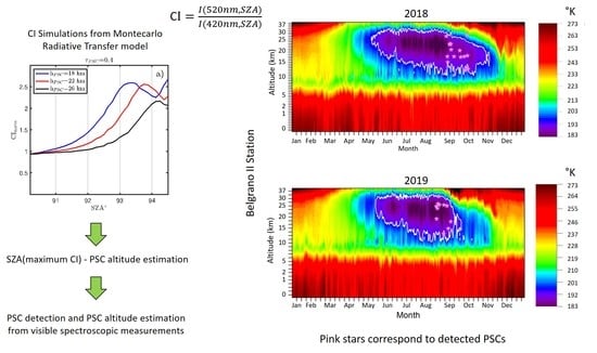
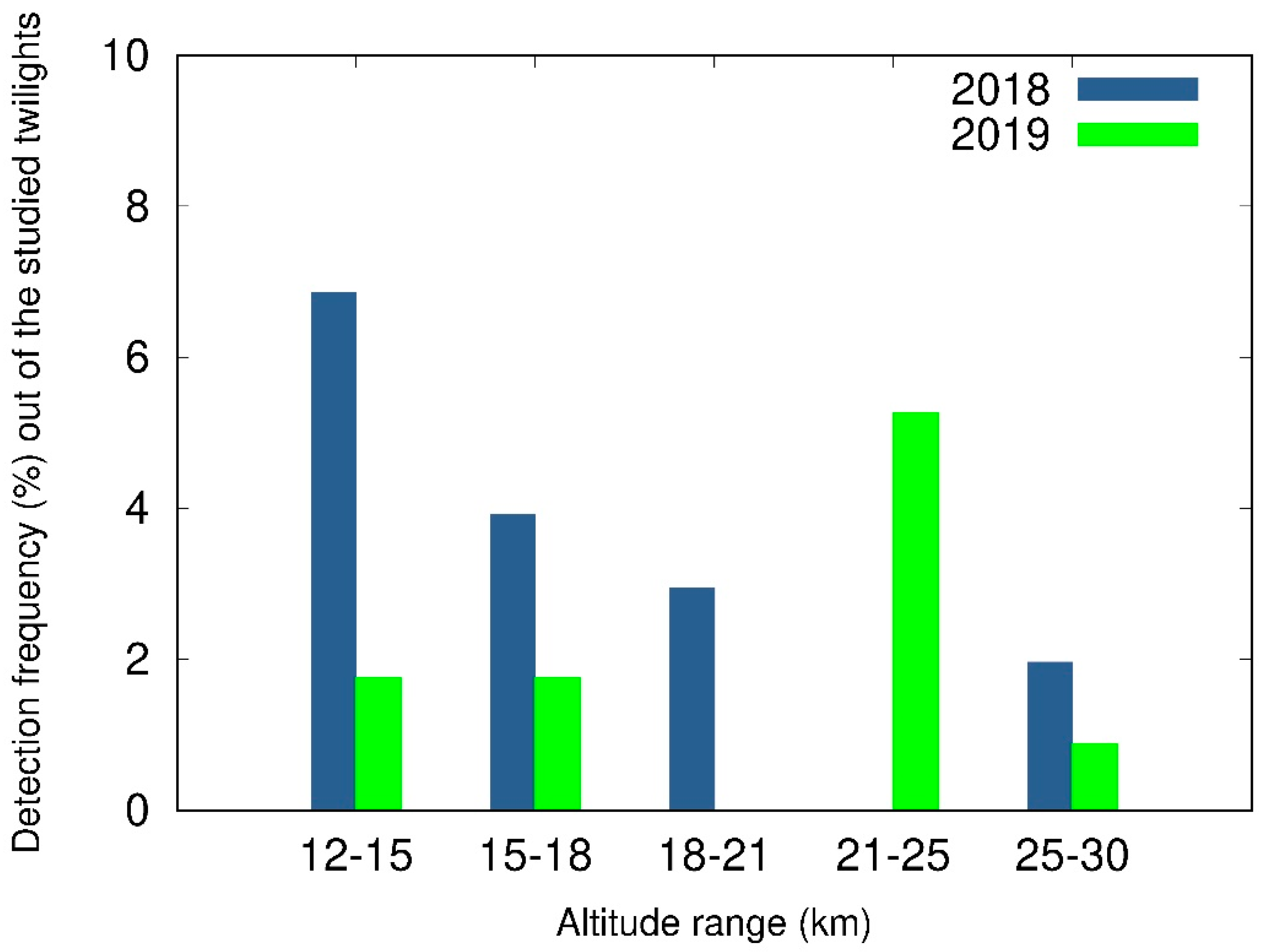
3.1. PSCs Detection at Belgrano II Station through Remote Sensing

To detect and characterize PSCs over Belgrano II, the CI evolution obtained from observations performed at zenith with the Vis DOAS instrument has been studied from mid-August to mid-October of 2018 and 2019. This period corresponds to the coldest period of the Austral winter, when the polar vortex over Antarctica is most stable, and thus the formation of PSCs is more probable [47,48]. Daily mean distance from the polar vortex edge to Belgrano II station, obtained from 1999 to 2011, shows that this station is continuously inside the vortex from beginning of June until the end of November [48]. Note that Vis scattered sunlight DOAS observations for the SZAs considered herein, are only available from 26 August 2018 and from 15 August 2019.
As shown with the RTM, the presence of PSC is evidenced as a maximum on the CI evolution during twilight. In order to emphasize this signature, the CI of each day is normalized using CI evolution of a considered Rayleigh day (RD, i.e., a day with no presence of tropospheric clouds or PSCs). Using meteorological observations performed on-site for the considered periods, we have chosen 24 September 2019 as RD for the normalization of the data. Among all clear days over Belgrano II for the considered period, experimental CI evolution observed on this day is the most similar to a modeled RD and presents one of the most stable behaviors (absence of clouds all along the day). Note that in previous works [35], the value of the CI at SZA = 90°, CI90, is used instead of CIRD for CI normalization. However, the presence of tropospheric clouds could produce a large value of CI90, sometimes as high as the relative maxima produced by PSCs. Thus, by normalizing with CI90, PSCs signatures could be masked and so their detection. In addition, by normalizing by the CI signal measured for a RD, the PSCs signature on the CI evolution is much more pronounced than by using CI90, making much easier the detection.
As concluded from the RTM simulations, the altitude of the PSC (hPSC) can be estimated from the SZA at which the CI maximum is presented (SZAmax). A relationship between hPSC and SZAmax have been obtained by fitting the model results with a second order polynomial (see Figure 5). These results indicate that clouds with altitudes below 12 km present CInorm maxima for SZA lower than 92°. Thus, a PSC detection case is considered in this work if the CInorm evolution presents a local maximum for SZA higher than 92°.
Figure 8 shows the temporal variation of atmospheric temperature profiles over Belgrano II, along with the altitudes of PSCs detected on years (a) 2018 and (b) 2019 (pink stars). As it can be observed, in 2019 the detection of PSCs practically stops on 12 September (Julian day 255), while in 2018 the presence of PSCs extends over the whole period studied. This is in a good agreement with the temperature data presented in the same figure. Note that in 2019 a sudden stratospheric warming event took place above Antarctica on September [54]. In Figure 8, white contour outlines the altitudes and time of temperatures lower than 195 K (−78 °C), where PSCs usually may form. Note that on 2 October 2018, a PSC has been detected outside this contour, at temperatures around 207.5 K (−65.5 °C), at an estimated altitude of 28.2 km. The formation of PSCs at these temperatures is very scarce (that must be seen as a singularity) but not impossible [3]. In addition, the error of the estimation of the PSC altitude increases with altitude (errors up to 3 km for the highest hPSC, and only 0.2 km for the lowest hPSC observed). The reason for that is that experimental measurements are more separated in time as higher is the SZA, since the intensity of the light reaching the instrument is lower as higher is this angle. Thus, a higher integration time has to be used to record the measurement. If error bars are estimated thought the SZA resolution at the maximum of CI, this PSC would be actually located between 28.2 − 1.8 and 28.2 + 2.9 km. Figure 8b shows that common temperature conditions for PSC formation (white contour) were only present until the first days of September 2019. In 2018, on the other hand, low temperatures remained present until the end of October. However, from the beginning of September 2018, altitude of the minimum temperature experimented a significant decrease. This feature can also be observed in our data. Figure 8 (pink stars) shows that PSCs are detected all over the considered period, but the hpsc of 2018 decreases notably from 12 September (except for an isolated case on 2 October), and PSCs detection in 2019 practically stops on that date. From 26 August to 15 October, a total number of 18 PSCs were detected in 2018, while in 2019 only 4 PSCs were detected during the same period. Thus, our observations confirm that the different temperature pattern during 2018 vs. 2019 above Belgrano during the polar sunrise resulted in less PSCs in 2019. Recent works have indeed confirmed 2019 as the year with the smallest Antarctic ozone hole on records [55,56].
To study the altitude of the PSCs in the considered periods, following the relationship between hPSC vs. SZAmax obtained with the model, PSCs detected on each year have been classified in five groups: hPSC = (12–15) km, hPSC = (15–18) km, hPSC = (18–21) km, hPSC = (21–25) km, and hPSC = (25–30) km. In 2018, most of the detected PSCs had altitudes below 15 km, with a frequency of occurrence of 7% out of the 102 twilights of the considered period (Figure 9). This frequency decreases with increasing altitude, being of only 2% for PSCs between 25 and 30 km. Note that the altitude of minimum temperature shown in Figure 8, for the considered period, decreases with time. On the contrary, most of the PSCs detected in 2019 had altitudes ranging from 21 to 25 km, with an occurrence frequency of 5% out of 114 twilights. The temporal evolution of lowest temperature in this case remains constant during most of August, and then decrease rapidly from the beginning to 12 September, approximately, which can be also observed in our results.

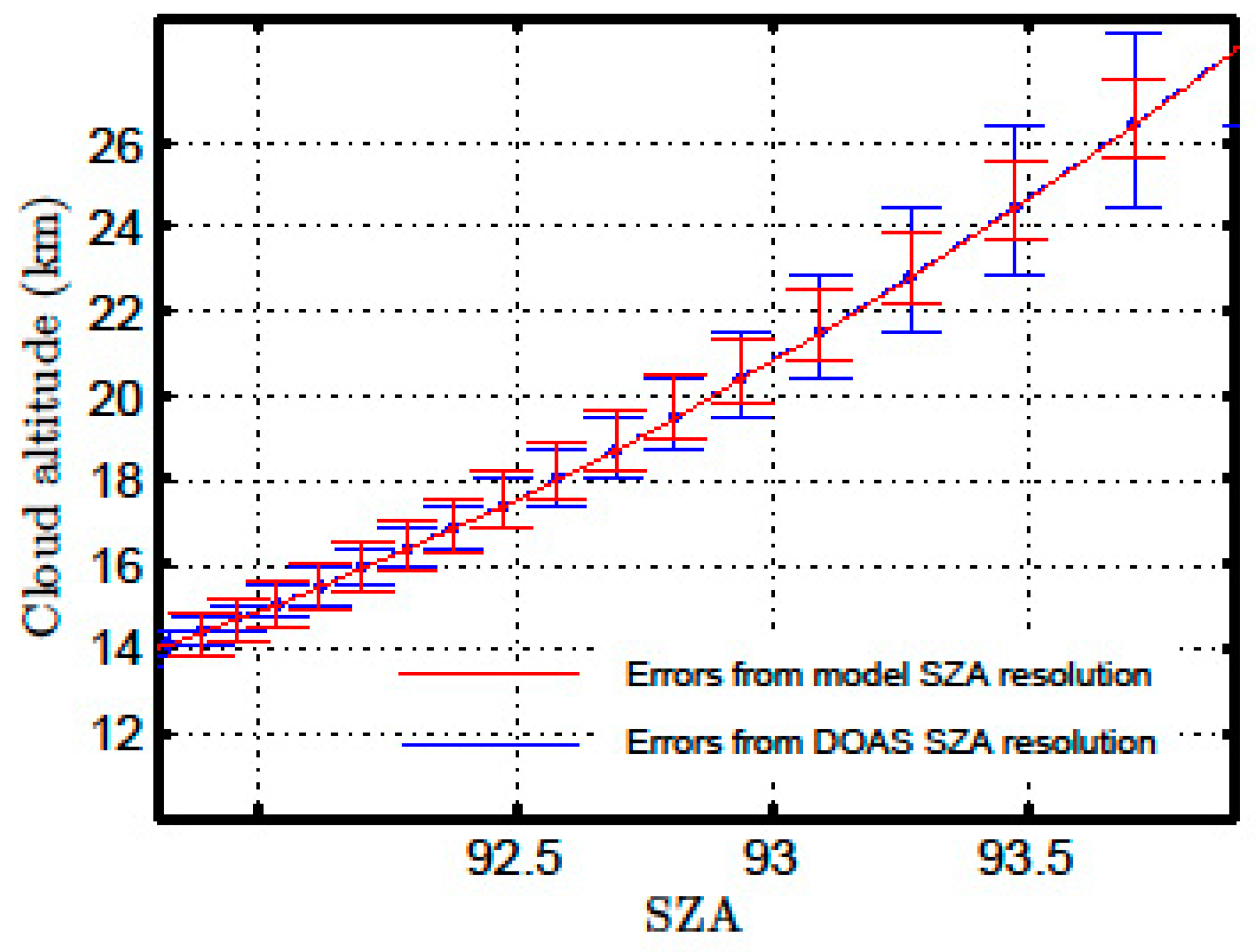
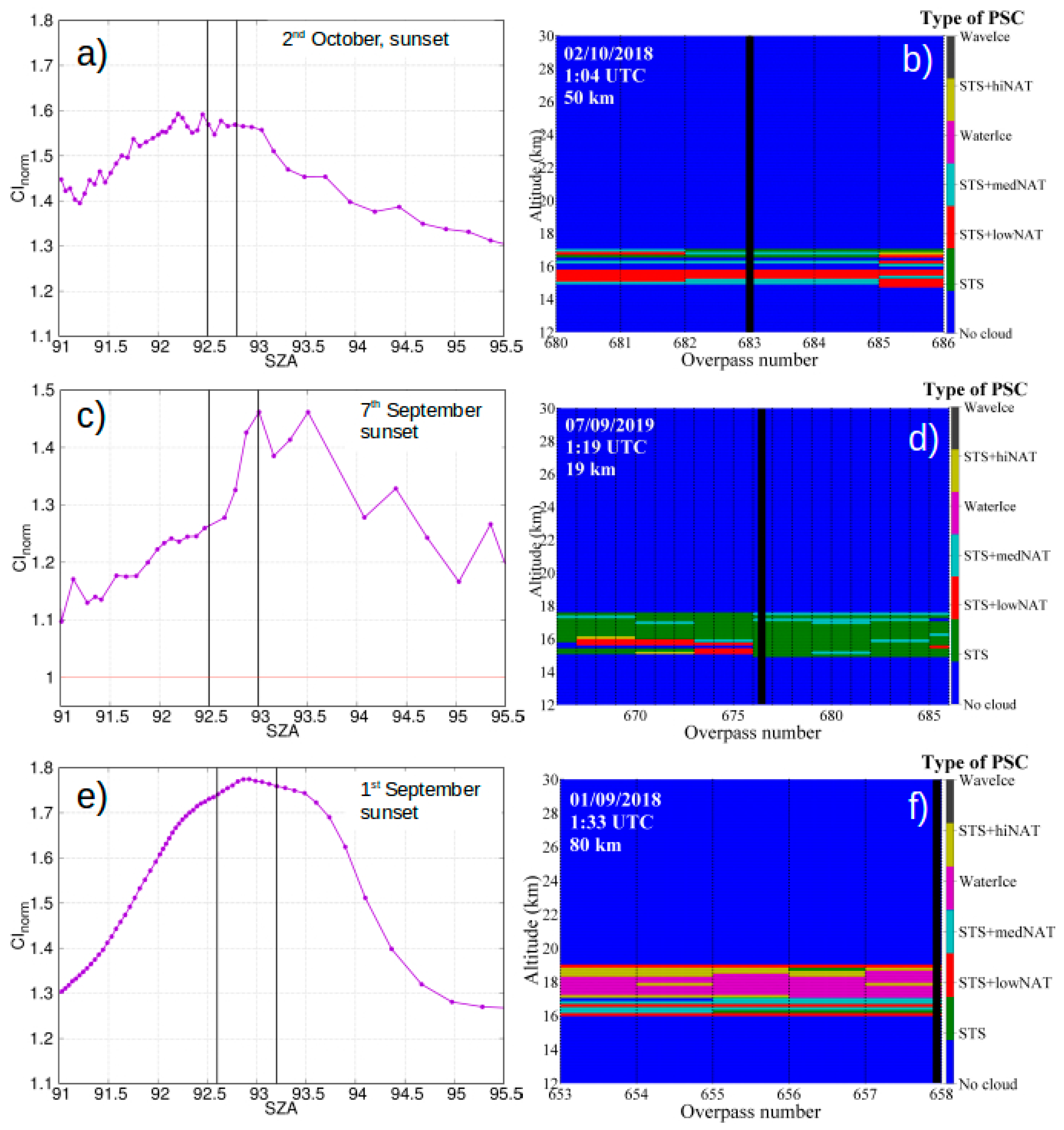
3.2. PSC Characterization in UV Spectral Range

As mentioned previously in Section 2.1, in addition to the shown Vis observations, NEVA II also measures spectra in the UV spectral range. In order to validate the CI approach for PSC detection in the UV range, similar simulations as in Section 2 were performed for λ1 = 401 nm and λ2 = 332.5 nm (wavelengths selected to minimize the absorption of gases in this range). Figure 10 shows, as example, the variation of SZAmax with PSC altitude computed for these two wavelengths, a cloud opacity τPSC = 0.2 and the gas profiles given in Figure 4 for October. Our results indicate that, due to the higher Rayleigh opacity in the UV wavelength range: (a) there is a change in the hPSC-SZA curve respect to the Vis case shown in Figure 5; (b) PSC clouds at altitudes lower than ~20 km cannot be detected in the UV spectral range (the simulations did not show any CI maximum in these case).
Although our simulations show that UV range is not the most appropriate for the detection of PSCs, observations in this range allows to cross validate between a PSC detection case above 20 km and the hPSC-SZA curves shown in Figure 5 (Vis channel) and Figure 10 (UV). Figure 11 shows, as example, CInorm signals measured on 2 October 2018 at the bands used in Figure 5 (Vis) and Figure 10 (UV). These CInorm signals, along with the hPSC-SZA curves, provide PSCs altitudes of 25.7 ± 1.8 km (UV) and 28.2 ± 1.8 km (Vis). The error bars were estimated thought the SZA resolution at the maximum of CI.
Therefore, we conclude that both spectrometers provide consistent PSC altitudes and that, although CInorm in UV range is not the most suitable parameter for PSC detection and characterization, it allows to validate the results given in the Vis spectral range (Figure 5).

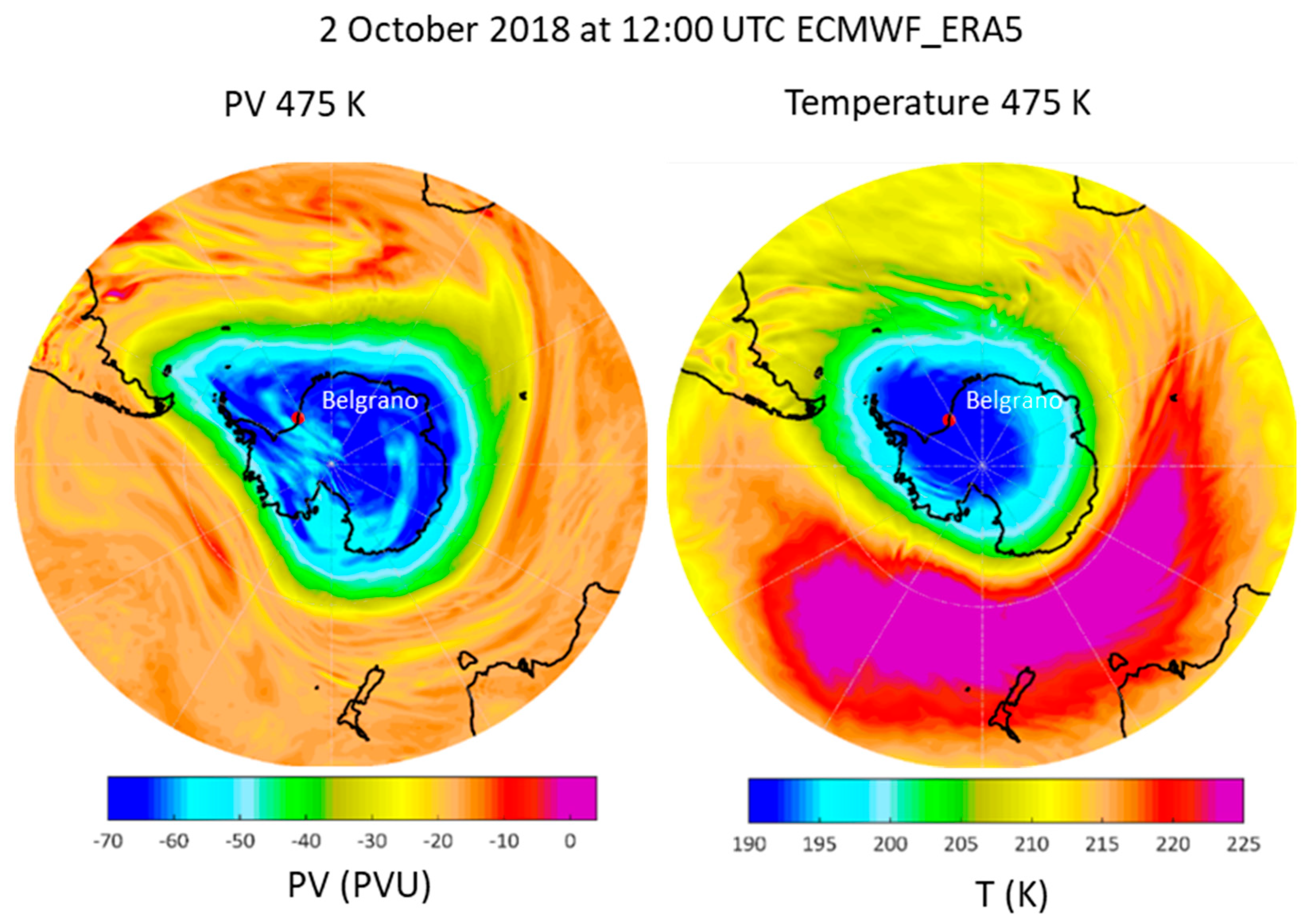
3.3. Comparison of Ground-Based and Satellite Observations

In this section, selected days are chosen for comparing the results obtained by the ground-based observations with those performed by CALIOP. As mentioned before, in the presence of a PSC, most of the scattered light reaching our instrument (pointing at zenith) comes from the cloud just above the light collector (i.e., zenith direction). Thus, the CALIOP data considered for this comparison exercise are for satellite overpasses close to the ground-based site (≤50 km). Note that the PSC-CALIOP product relates to nighttime orbits [19] while the ground-based instrument needs scattered skylight during twilight. Therefore, most of the times DOAS and CALIOP measurements are not simultaneous. However, this comparison, used here as a cross-check of the PSC detection method, relies on the geographical and temporal stability of the PSCs once formed inside a stable polar vortex (e.g., [4,22]). Based on this assumption, former studies have compared ground-based and satellite lidar observations within 100 km from the ground-based site (e.g., [4]). Thus, our distance threshold for ground-based/satellite comparison is indeed quite conservative since the horizontal extension of PSCs has been reported of up to 200 km in the less stable Arctic polar vortex [6].
For this cross-check, only PSCs detected by CALIPSO presenting a stable form over the satellite overpass have been taken into account. CALIPSO PSC detection cases under the presence of thick tropospheric clouds have been also discarded from this comparison. Under these conditions, we found a good agreement between the altitudes of the PSCs observed by CALIPSO and the PSCs detected in this work. In Figure 12, some examples of PSCs detected by CALIPSO are compared with the evolution of the CInorm obtained from our ground-based spectrometer. In these CI plots, the black lines indicate SZAs corresponding to altitudes of the base and the top of the PSCs as detected by CALIPSO (following the functions of Figure 5). These results indicate that PSC altitudes derived by both techniques are in good agreement. Note that only for Figure 12f the CALIPSO overpass exceeds the threshold of 50 km (80 km). This day, there are not overpasses within the 50 km from the station, but the CI shows a clear maximum. Thus, we looked for a possible overpass of the satellite that could observe this cloud, as it was confirmed. This supports also that the selected distance threshold between the satellite overpass and our research site, chosen in this work as 50 km, is a conservative value. This exercise strengthen the consistency of the results obtained by the CI with the ground-based instrumentation.

4. Conclusions

Based on the work of Sarkissian et al. 1991 [32], we have studied the evolution of a normalized CI during twilight to detect and characterize PSCs over the Belgrano II Antarctic station, during 2018 and 2019. In this work, we have shown that using a spectral range half-shorter than previous works, we are still able to detect PSCs and estimate their altitude. This means that instruments that are (or were) not meant initially for investigating PSCs, such as the ground-based UV/Vis spectrometers that belong to the NDACC network in both polar regions, or the MAX-DOAS instruments on board research vessels in the polar regions, could perform this sort of research. Concerning NDACC in polar regions, currently there are 14 stations with UV/VIS spectrometers and only six with lidars (https://www.ndacc.org/, accessed on 25 February 2021). Therefore, even though lidars provide more detailed information on the vertical PSC distribution than the UV/Vis spectrometers as the one used in this work, the method used in this work offers the possibility for other sort of instruments to contribute to a better understanding of the PSCs throughout both polar regions.
Regarding the novelty of the method presented in this study, it is worth noting that previous works using similar CI methods for the PSC detection were based on the results obtained by a single scattering RTM [32,35,36,37]. In this work, we have used a full spherical multiple scattering model which is more suitable for the large optical paths or high scattering media considered here than single scattering pseudo-spherical models. These simulations allow us to better characterize the effects of PSC on the CI signals computed from our instrument observations. Moreover, we have also defined which parameters can be determined by studying the CI evolution (i.e., altitude) and which ones cannot (i.e., optical properties), or which variables play a significant role on the observations. While the shape of the CI maximum depends, among other parameters, on the PSC particle properties or the presence of tropospheric clouds, the results shown in Section 2.4.3 indicate that the SZA of maximum CI mainly depends on the PSC altitude (even under the presence of tropospheric cloud). As a result, in our analysis only PSC altitude could be inferred.
Our CI approach has been applied to measurements performed at Belgrano II with an optical spectrometer measuring in the visible spectral range during the coldest days of the austral winter of 2018 and 2019. Results show that the frequency and altitude of the PSCs in 2019 were lower than in 2018, consistent also with the sudden stratospheric even of 2019. The detected PSCs and their estimated altitude inferred in this work are in good agreement with the temperature profiles of the ECMWF and with the PSCs observed by CALIPSO. In addition, a similar CI method at UV range has also been studied. Results show that the UV range is much more limited than the Vis to study PSCs since in the UV PSCs are detected only if they are located above an altitude of 20 kms. The UV range has been used herein to verify the method proposed for the visible spectral range.
Note, also, that zenith-DOAS instruments, like the one used in this study, are traditionally used to measure trace gases concentrations integrated over the optical path (known as differential Slant Column Densities [43]). Using the CI approach presented in this work, zenith-DOAS measurements can be used to relate the stratospheric polar chemistry they are originally targeted to investigate, with the presence of PSCs. In future works, we will perform such a study. We will also apply the detection and characterization of PSCs to a larger record of measurements (several years) for different polar stations, which will allow for a better spatial characterization of PSCs.

Author Contributions

Conceptualization, L.G.-M., D.T., C.P.-R. and M.Y.; methodology, L.G.-M. and D.T.; software, L.G.-M. and D.T.; validation, L.G.-M., D.T. and C.P.-R.; formal analysis, L.G.-M. and D.T.; investigation, L.G.-M., D.T., C.P.-R., M.Y. and J.A.A.; resources, M.Y. and H.O.; data curation, L.G.-M., D.T., C.P.-R., M.Y. and J.A.A.; writing—original draft preparation, L.G.-M., D.T. and C.P.-R.; writing—review and editing, L.G.-M., D.T., C.P.-R., M.Y. and J.A.A.; visualization, L.G.-M., D.T., C.P.-R. and J.A.A.; supervision, M.Y.; project administration, M.Y.; funding acquisition, M.Y. Please turn to the CRediT taxonomy for the term explanation. All authors have read and agreed to the published version of the manuscript.

Funding

This work was funded by the Spanish Ministry of Science and Innovation under the projects VHODCA (CTM2017-83199P).

Institutional Review Board Statement

Not applicable.

Informed Consent Statement

Not applicable.

Data Availability Statement

The data presented in this study are available on request from Margarita Yela.

Acknowledgments

The CALIOP-Calipso data were obtained through the Earthdata Search site from the NASA Langley Research Center–Atmospheric Science Data Center (doi: 10.5067/CALIOP/CALIPSO/CAL_LID_L2_PSCMask-Prov-V1-00_L2-001.00). The authors thank the ECMWF (European Centre for Medium-Range Weather Forecasts) for the ERA5 meteorological fields, and the AEMET (Spanish State Meteorological Agency) for granting access to the services of the ECMWF. The authors would also acknowledge the work done by the different technicians at the station of Belgrano.

Conflicts of Interest

The authors declare no conflict of interest.

References

  1. Spang, R.; Hoffmann, L.; Muller, R.; Grooß, J.U.; Tritscher, I.; Hopfner, M.; Pitts, M.; Orr, A.; Riese, M. A climatology of polar stratospheric cloud composition between 2002 and 2012 based on MIPAS/Envisat observations. Atmos. Chem. Phys. 2018, 18, 5089–5113. [Google Scholar] [CrossRef] [Green Version]
  2. Hanson, D.; Mauersberger, K. Laboratory studies of the nitric acid trihydrate: Implications for the south polar stratosphere. Geophys. Res. Lett. 1988, 15, 855–858. [Google Scholar] [CrossRef]
  3. Noel, V.; Hertzog, A.; Chepfer, H.; Winker, D.M. Polar stratospheric clouds over Antarctica from the CALIPSO spaceborne lidar. J. Geophys. Res. Atmos. 2008, 113, D02205. [Google Scholar] [CrossRef] [Green Version]
  4. Snels, M.; Scoccione, A.; Di Liberto, L.; Colao, F.; Pitts, M.; Poole, L.; Deshler, T.; Cairo, F.; Cagnazzo, C.; Fierli, F. Comparison of Antarctic polar stratospheric cloud observations by ground-based and space-borne lidar and relevance for chemistry-climate models. Atmos. Chem. Phys. 2019, 19, 955–972. [Google Scholar] [CrossRef] [Green Version]
  5. Larsen, N.; Knudsen, B.M.; Rosen, J.M.; Kjome, N.T.; Neuber, R.; Kyro, E. Temperature histories in liquid and solid polar stratospheric cloud formation. J. Geophys. Res. 1997, 102, 23505–23517. [Google Scholar] [CrossRef] [Green Version]
  6. Schreiner, J.; JSchreiner, J.; Voigt, C.; Weisser, C.; Kohlmann, A.; Mauersberger, K.; Deshler, T.; Kröger, C.; Rosen, J.; Larsen, N.; et al. Chemical, microphysical, and optical properties of polar stratospheric clouds. J. Geophys. Res. 2003, 108, 8313. [Google Scholar] [CrossRef]
  7. Von Hobe, M.; Bekki, S.; Borrmann, S.; Cairo, F.; D’Amato, F.; Di Donfrancesco, G.; Dörnbrack, A.; Ebersoldt, A.; Ebert, M.; Emde, C.; et al. Reconciliation of essential process parameters for an enhanced predictability of Arctic stratospheric ozone loss and its climate interactions (RECONCILE): Activities and results. Atmos. Chem. Phys. 2013, 13, 9233–9268. [Google Scholar] [CrossRef] [Green Version]
  8. Von Savigny, C.; Ulasi, E.P.; Eichmann, K.-U.; Bovensmann, H.; Burrows, J.P. Detection and mapping of polar stratospheric clouds using limb scattering observations. Atmos. Chem. Phys. 2005, 5, 3071–3079. [Google Scholar] [CrossRef]
  9. Vanhellemont, F.; Fussen, D.; Mateshvili, N.; Tétard, C.; Bingen, C.; Dekemper, E.; Loodts, N.; Kyrölä, E.; Sofieva, V.; Tamminen, J.; et al. Optical extinction by upper tropospheric/stratospheric aerosols and clouds: GOMOS observations for the period 2002–2008. Atmos. Chem. Phys. 2010, 10, 7997–8009. [Google Scholar] [CrossRef] [Green Version]
  10. Taylor, F.W.; Lambert, A.; Grainger, R.G.; Rodgers, C.D.; Remedios, J.J. Properties of Northern Hemisphere Polar Stratospheric Clouds and Volcanic Aerosol in 1991/2 from UARS/ISAMS Satellite Measurements. J. Atmos. Sci. 1994, 51, 3019–3026. [Google Scholar] [CrossRef] [Green Version]
  11. Massie, S.T.; Bailey, P.L.; Gille, J.C.; Lee, E.C.; Mergenthaler, J.L.; Roche, A.E.; Kumer, J.B.; Fishbein, E.F.; Waters, J.W.; Lahoz, W.A. Spectral signatures of polar stratospheric clouds and sulfate aerosol. J. Atmos. Sci. 1994, 51, 3027–3044. [Google Scholar] [CrossRef] [Green Version]
  12. Spang, R.; Remedios, J. Observations of a distinctive infra-red spectral feature in the atmospheric spectra of polar stratospheric clouds measured by the CRISTA instrument. Geophys. Res. Lett. 2003, 30, 1875. [Google Scholar] [CrossRef] [Green Version]
  13. Fischer, H.; Birk, M.; Blom, C.; Carli, B.; Carlotti, M.; von Clarmann, T.; Delbouille, L.; Dudhia, A.; Ehhalt, D.; Endemann, M.; et al. MIPAS: An instrument for atmospheric and climate research. Atmos. Chem. Phys. 2008, 8, 2151–2188. [Google Scholar] [CrossRef] [Green Version]
  14. Spang, R.; Riese, M.; Offermann, D. CRISTA-2 observations of the south polar vortex in winter 1997: A new data set for polar process studies. Geophys. Res. Lett. 2001, 28, 3159–3162. [Google Scholar] [CrossRef]
  15. Spang, R.; Remedios, J.J.; Kramer, L.J.; Poole, L.R.; Fromm, M.D.; Müller, M.; Baumgarten, G.; Konopka, P. Polar stratospheric cloud observations by MIPAS on ENVISAT: Detection method, validation and analysis of the northern hemisphere winter 2002/2003. Atmos. Chem. Phys. 2005, 5, 679–692. [Google Scholar] [CrossRef] [Green Version]
  16. Spang, R.; Remedios, J.J.; Tilmes, S.; Riese, M. MIPAS observation of polar stratospheric clouds in the Arctic 2002/2003 and Antarctic 2003 winters. Adv. Space Res. 2005, 36, 868–878. [Google Scholar] [CrossRef]
  17. Winker, D.M.; Vaughan, M.A.; Omar, A.; Hu, Y.X.; Powell, K.A.; Liu, Z.Y.; Hunt, W.H.; Young, S.A. Overview of the CALIPSO Mission and CALIOP Data Processing Algorithms. J. Atmos. Ocean. Technol. 2009, 26, 2310–2323. [Google Scholar] [CrossRef]
  18. Pitts, M.C.; Thomason, L.W.; Poole, L.R.; Winker, D.M. Characterization of Polar Stratospheric Clouds with spaceborne lidar: CALIPSO and the 2006 Antarctic season. Atmos. Chem. Phys. 2007, 7, 5207–5228. [Google Scholar] [CrossRef] [Green Version]
  19. Pitts, M.C.; Poole, L.R.; Thomason, L.W. CALIPSO polar stratospheric cloud observations: Second-generation detection algorithm and composition discrimination. Atmos. Chem. Phys. 2009, 9, 7577–7589. [Google Scholar] [CrossRef] [Green Version]
  20. Pitts, M.C.; Poole, L.R.; Dörnbrack, A.; Thomason, L.W. The 2009–2010 Arctic polar stratospheric cloud season: A CALIPSO perspective. Atmos. Chem. Phys. 2011, 11, 2161–2177. [Google Scholar] [CrossRef] [Green Version]
  21. Pitts, M.C.; Poole, L.R.; Lambert, A.; Thomason, L.W. An assessment of CALIOP polar stratospheric cloud composition classification. Atmos. Chem. Phys. 2013, 13, 2975–2988. [Google Scholar] [CrossRef] [Green Version]
  22. Campbell, J.R.; Sassen, K. Polar stratospheric clouds at the South Pole from 5 years of continuous lidar data: Macrophysical, optical, and thermodynamic properties. J. Geophys. Res. 2008, 113, D20204. [Google Scholar] [CrossRef]
  23. Adriani, A.; Deshler, T.; Gobbi, G.P.; Johnson, B.J.; Di Donfrancesco, G. Polar stratospheric clouds over McMurdo, Antarctica, during the 1991 spring: Lidar and particle counter measurements. Geophys. Res. Lett. 1992, 19, 1755–1758. [Google Scholar] [CrossRef] [Green Version]
  24. Adriani, A.; Deshler, T.; Di Donfrancesco, G.; Gobbi, G. Polar stratospheric clouds and volcanic aerosol during spring 1992 over McMurdo Station, Antarctica: Lidar and particle counter comparative measurements. J. Geophys. Res. Atmos. 1995, 100, 25877–25897. [Google Scholar] [CrossRef] [Green Version]
  25. Adriani, A.; Massoli, P.; Di Donfrancesco, G.; Cairo, F.; Moriconi, M.; Snels, M. Climatology of polar stratospheric clouds based on lidar observations from 1993 to 2001 over McMurdo Station, Antarctica. J. Geophys. Res. Atmos. 2004, 109, D24211. [Google Scholar] [CrossRef] [Green Version]
  26. Di Liberto, L.; Cairo, F.; Fierli, F.; Di Donfrancesco, G.; Viterbini, M.; Deshler, T.; Snels, M. Observation of polar stratospheric clouds over McMurdo (77.85° S, 166.67° E) (2006–2010). J. Geophys. Res. Atmos. 2014, 119, 5528–5541. [Google Scholar] [CrossRef] [Green Version]
  27. Córdoba-Jabonero, C.; Guerrero-Rascado, J.L.; Toledo, D.; Parrondo, M.; Yela, M.; Gil, M.; Ochoa, H.A. Depolarization ratio of polar stratospheric clouds in coastal Antarctica: Comparison analysis between ground-based Micro Pulse Lidar and spaceborne CALIOP observations. Atmos. Meas. Tech. 2013, 6, 703–717. [Google Scholar] [CrossRef] [Green Version]
  28. Santacesaria, V.; MacKenzie, A.R.; Stefanutti, L. A climatological study of polar stratospheric clouds (1989–1997) from LIDAR measurements over Dumont d’Urville (Antarctica). Tellus B 2001, 53, 306–321. [Google Scholar]
  29. David, C.; Bekki, S.; Godin, S.; Megie, G.; Chipperfield, M. Polar stratospheric clouds climatology over Dumont d’Urville between 1989 and 1993 and the influence of volcanic aerosols on their formation. J. Geophys. Res. Atmos. 1998, 103, 22163–22180. [Google Scholar] [CrossRef]
  30. David, C.; Keckhut, P.; Armetta, A.; Jumelet, J.; Snels, M.; Marchand, M.; Bekki, S. Radiosonde stratospheric temperatures at Dumont d’Urville (Antarctica): Trends and link with polar stratospheric clouds. Atmos. Chem. Phys. 2010, 10, 3813–3825. [Google Scholar] [CrossRef] [Green Version]
  31. Tesche, M.; Achtert, P.; Pitts, M.C. On the best locations for ground-based polar stratospheric cloud (PSC) observations. Atmos. Chem. Phys. 2021, 21, 505–516. [Google Scholar] [CrossRef]
  32. Sarkissian, A.; Pommereau, J.-P.; Goutail, F. Identification of polar stratospheric clouds from the ground by visible spectrometry. Geophys. Res. Lett. 1991, 18, 779–782. [Google Scholar] [CrossRef]
  33. Bohren, C.F.; Huffman, D.R. Absorption and Scattering of Light by Small Particles; John Wiley and Sons, Inc.: New York, NY, USA, 1983. [Google Scholar]
  34. Young, A.T. Rayleigh scattering. Appl. Opt. 1981, 20, 533–535. [Google Scholar] [CrossRef] [PubMed]
  35. Sarkissian, A.; Pommereau, J.; Goutail, F.; Kyro, E. PSC and volcanic aerosol observations during EASOE by UV-visible ground-based spectrometry. Geophys. Res. Lett. 1994, 21, 1319–1322. [Google Scholar] [CrossRef]
  36. Enell, C.-F.; Steen, A.; Wagner, T.; Frieß, U.; Platt, U. Occurrence of polar stratospheric clouds at Kiruna. Ann. Geophys. 1999, 17, 1457–1462. [Google Scholar] [CrossRef]
  37. Enell, C.F.; Stebel, K.; Wagner, T.; Frieß, U.; Pfeilsticker, K.; Platt, U. Detecting Polar Stratospheric Clouds with Zenith-Looking Photometers. Sodank. Geophys. Obs. Publ. 2003, 92, 55–59. [Google Scholar]
  38. Tran, T. Optical Depth Sensor for Measurement of Dust and Clouds in the Atmosphere of Mars: Radiative Transfer Simulations and Validation on Earth. Ph.D. Thesis, Université Versailles Saint-Quentin-en-Yvelines, Paris, France, 2005. [Google Scholar]
  39. Toledo, D.; Rannou, P.; Pommereau, J.; Sarkissian, A.; Foujols, T. Measurement of aerosol optical depth and sub-visual cloud detection us- ing the optical depth sensor (ODS). Atmos. Meas. Tech. 2016, 9, 455–467. [Google Scholar] [CrossRef] [Green Version]
  40. Toledo, D.; Rannou, P.; Pommereau, J.-P.; Foujols, T. The optical depth sensor (ODS) for column dust opacity measurements and cloud detection on martian atmosphere. Exp. Astron. 2016, 42, 61–83. [Google Scholar] [CrossRef]
  41. Toledo, D.; Arruego, I.; Apestigue, V.; Jimenez, J.; Gomez, L.; Yela, M.; Rannou, P.; Pommereau, J.-P. Measurement of dust optical depth using the solar irradiance sensor (SIS) onboard the ExoMars 2016 EDM. Planet. Space Sci. 2017, 138, 33–43. [Google Scholar] [CrossRef]
  42. Hönninger, G.; von Friedeburg, C.; Platt, U. Multi axis differential optical absorption spectroscopy (MAX DOAS). Atmos. Chem. Phys. 2004, 4, 231–254. [Google Scholar] [CrossRef] [Green Version]
  43. Platt, G.; Stutz, J. Differential Optical Absorption Spectroscopy (DOAS)—Principles and Applications; Springer Verlag: Heidelberg, Germany, 2008. [Google Scholar]
  44. Yela, M.; Gil-Ojeda, M.; Navarro-Comas, M.; González-Bartolomé, D.; Puentedura, O.; Funke, B.; Iglesias, J.; Rodríguez, S.; García, O.; Ochoa, H.; et al. Hemispheric asymmetry in stratospheric NO2 trends. Atmos. Chem. Phys. 2017, 17, 13373–13389. [Google Scholar] [CrossRef] [Green Version]
  45. Prados-Roman, C.; Gómez-Martín, L.; Puentedura, O.; Navarro-Comas, M.; Iglesias, J.; De Mingo, J.R.; Péreza, M.; Ochoa, H.; Barlasina, M.E.; Carbajal, G.; et al. Reactive bromine in the low troposphere of Antarctica: Estimations at two research sites. Atmos. Chem. Phys. 2018, 18, 8549–8570. [Google Scholar] [CrossRef] [Green Version]
  46. Parrondo, M.C.; Yela, M.; Gil, M.; von der Gathen, P.; Ochoa, H. Mid-winter lower stratosphere temperatures in the Antarctic vortex: Comparison between observations and ECMWF and NCEP operational models. Atmos. Chem. Phys. 2007, 7, 435–441. [Google Scholar] [CrossRef] [Green Version]
  47. Yela, M.; Parrondo, C.; Gil, M.; Rodriguez, S.; Araujo, J.; Ochoa, H.; Deferrari, G.; Diaz, S. The September 2002 Antarctic vortex major warmings as observed by visible spectroscopy and ozone soundings. Int. J. Remote Sens. 2005, 26, 3361–3376. [Google Scholar] [CrossRef]
  48. Parrondo, M.C.; Gil, M.; Yela, M.; Johnson, B.J.; Ochoa, H. Antarctic ozone variability inside the polar vortex estimated from balloon measurements. Atmos. Chem. Phys. 2014, 14, 217–229. [Google Scholar] [CrossRef] [Green Version]
  49. Hersbach, H.; Bell, B.; Berrisford, P.; Hirahara, S.; Horányi, A.; Muñoz-Sabater, J.; Nicolas, J.; Peubey, C.; Radu, R.; Schepers, D.; et al. The ERA5 global reanalysis. Q. J. R. Meteorol. Soc. 2020, 146, 1999–2049. [Google Scholar] [CrossRef]
  50. Chance, K.V.; Spurr, R.J.D. Ring effect studies: Rayleigh scattering, including molecular parameters for rotational Raman scattering, and the Fraunhofer spectrum. Appl. Optics 1997, 36, 5224–5230. [Google Scholar] [CrossRef] [PubMed] [Green Version]
  51. Anderson, G.P.; Clough, S.A.; Kneizys, F.X.; Chetwynd, J.H.; Shettle, E.P. AFGL Atmospheric Constituent Profiles (0.120 km); Tech. Rep., AFGL-TR-86-0110, Environemental Research Papers No. 954; Air Force Geophysics Laboratory, Hanscom Air Force Base: Bedford, MA, USA, 1986. [Google Scholar]
  52. Burrows, J.P.; Dehn, A.; Deters, B.; Himmelmann, S.; Richter, A.; Voigt, S.; Orphal, J. Atmospheric remote-sensing reference data from GOME: Part1. Temperature-dependent absorption cross-section of NO2 in the 231–794 nm range. J. Quant. Spectrosc. Radiat. Transf. 1998, 60, 1025–1031. [Google Scholar] [CrossRef]
  53. Molina, L.T.; Molina, L.J. Absolute absorption cross sections of ozone in the 185- to 350-nm wavelength range. J. Geophys. Res. 1986, 91, 14501–14508. [Google Scholar] [CrossRef]
  54. Safieddine, S.; Bouillon, M.; Paracho, A.C.; Jumelet, J.; Tencé, F.; Pazmino, A.; Goutail, F.; Wespes, C.; Bekki, S.; Boynard, A.; et al. Antarctic Ozone Enhancement During the 2019 Sudden Stratospheric Warming Event. Geophys. Res. Lett. 2020, 47, e2020GL087810. [Google Scholar] [CrossRef]
  55. Krummel, P.; Fraser, P. The 2019 Antarctic Ozone Hole. Report #12; Wednesday 13 November 2019; Climate Science Centre, CSIRO Oceans and Atmosphere: Aspendale, Australia, 2019. [Google Scholar]
  56. Amos, M.; Young, P.J.; Hosking, J.S.; Lamarque, J.-F.; Abraham, N.L.; Akiyoshi, H.; Archibald, A.T.; Bekki, S.; Deushi, M.; Jöckel, P.; et al. Projecting ozone hole recovery using an ensemble of chemistry-climate models weighted by model performance and independence. Atmos. Chem. Phys. 2020, 20, 9961–9977. [Google Scholar] [CrossRef]
Figure 1. Spatial distribution of PV (Pressure·Volume) and temperature in the Antarctic and surroundings at the 475 K isentropic level on 2 October 2018 at 12:00 UTC. The location of Belgrano II is indicated with a red dot over Antarctica. Edges of the vortex are usually considered at the highest PV gradients, which in this figure correspond to PV values around −40.
Remotesensing 13 01412 g001
Figure 2. (a) Simulated color index during twilight for a cloud opacity of τPSC = 0.4 and cloud altitude hPSC = 18, 22, 26, and 26 km, (b) Same as left panel but for hPSC = 22 km and τPSC = 0.05, 0.1, and 0.2.
Remotesensing 13 01412 g002
Figure 3. (a) Cloud phase functions computed using T-Matrix for different reff values and; (b) Simulated color index during twilight for the phase functions illustrated in previous panel and for hPSC = 22 km and τPSC = 0.2.
Remotesensing 13 01412 g003
Figure 4. Vertical profiles of (a) O3 and (b) NO2 concentrations at Belgrano II station during the months of August (blue), September (red) and October (black).
Remotesensing 13 01412 g004
Figure 5. Polar Stratospheric Clouds (PSC) altitude vs solar zenith angles (SZA) of maximum color index (CI) from simulations (blue) and its corresponding polynomial fitting (red), for the months of August (a), September (b) and October (c). The curves were computed for a PSC cloud opacity τPSC = 0.2, no tropospheric clouds and the gas profiles illustrated in Figure 4.
Remotesensing 13 01412 g005
Figure 6. SZAmax values obtained for different PSC altitudes under tropospheric cloud free conditions (red solid line) and when a tropospheric cloud layer with a total opacity of 1 is added at an altitude of 5 km (blue error bars). The errors were computed according to the model SZA resolution at the CI maximum.
Remotesensing 13 01412 g006
Figure 7. Comparison between the errors in cloud altitude of the Monte-Carlo radiative transfer model (RTM) (red) and the spectrometer (blue). In both cases the errors were computed from the SZA resolution at the maximum of CI.
Remotesensing 13 01412 g007
Figure 8. Temperatures profiles over Belgrano II obtained with ERA5 data reanalysis from the global meteorological model European Centre for Medium Range Weather Forecasts (ECMWF) (a) during 2018; and (b) during 2019. White contour outlines the altitudes and time of temperatures lower than −78 °C (195 K), where Polar Stratospheric Clouds usually may form. Pink stars correspond to the PSCs detected in this work.
Remotesensing 13 01412 g008
Figure 9. Occurrence frequency (out of the studied twilights) of derived altitudes in % (2018 in blue, 2019 in green) out of the number of studied twilights.
Remotesensing 13 01412 g009
Figure 10. Variation of the SZA of maximum CI with the cloud altitude in the UV spectral range. This curve was computed for λ1 = 401 nm and λ2 = 332.5 nm, a cloud opacity τPSC = 0.2, and the gas profiles illustrated in Figure 4 for the month of October. Simulations are shown in blue and the polynomial fit of the observations in red.
Remotesensing 13 01412 g010
Figure 11. CInorm evolution obtained from recorded spectra on 2 October 2018 (sunrise) for UV (violet) and visible (green) measurements. SZA corresponding to the CInorm maximums are marked by arrows.
Remotesensing 13 01412 g011
Figure 12. CInorm evolution vs. SZA obtained from our ground-based Vis spectrometer (left figures: a,c,e) and by Cloud-Aerosol-Lidar and Infrared Pathfinder Satellite Observations (CALIPSO) (right figures: b,d,f). The upper figures (a,b) correspond to observations performed on the sunset of 2 October 2018; the figures in the middle to observations performed on 7 September 2019; and the lower figures (e,f) to those on 1 September 2018. The color code of the CALIPSO figures correspond to the different types of PSCs as described in Section 2.2.
Remotesensing 13 01412 g012
Publisher’s Note: MDPI stays neutral with regard to jurisdictional claims in published maps and institutional affiliations.

