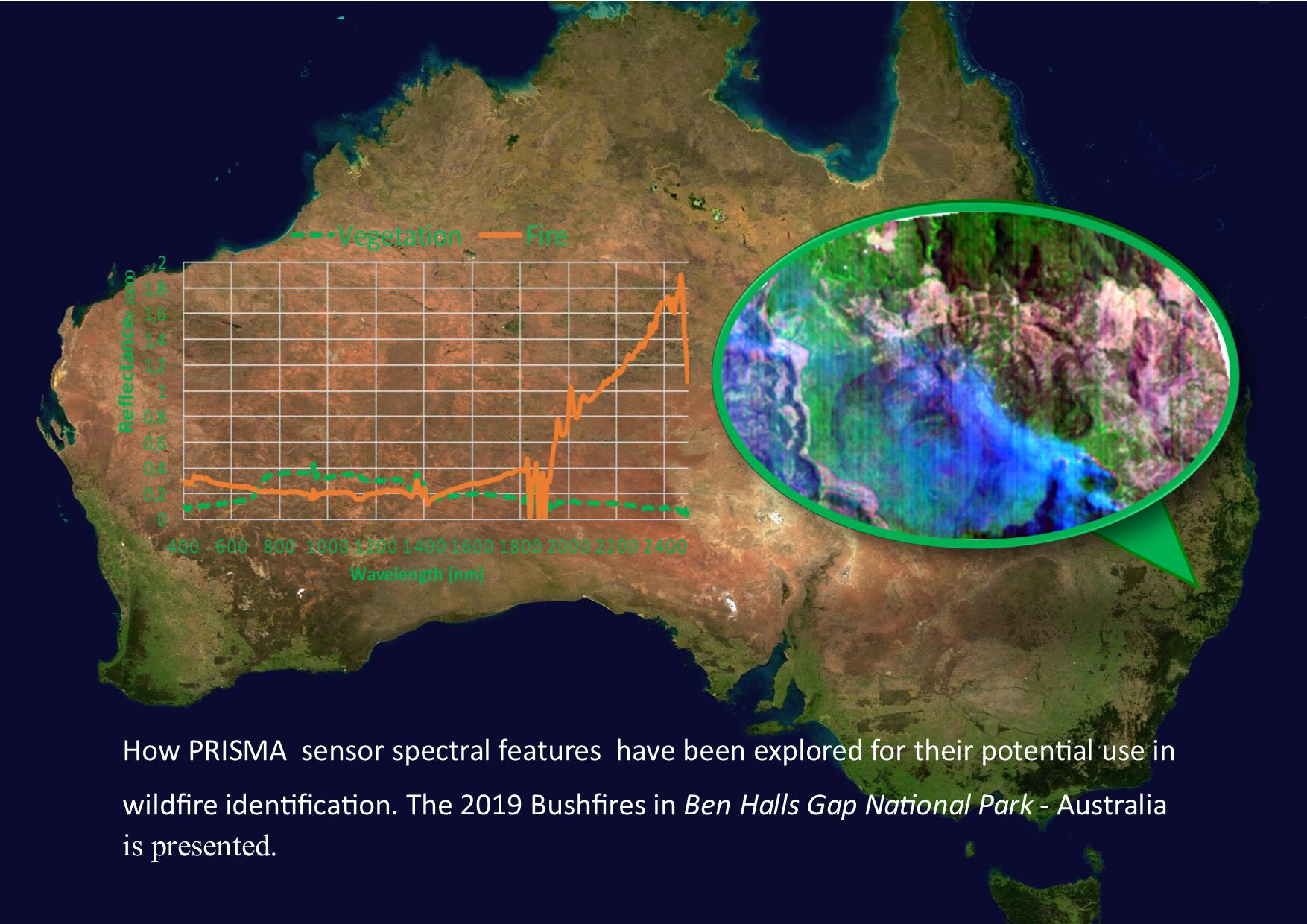
Exploring PRISMA Scene for Fire Detection: Case Study of 2019 Bushfires in Ben Halls Gap National Park, NSW, Australia

Abstract

Precursore IperSpettrale della Missione Applicativa (Hyperspectral Precursor of the Application Mission, PRISMA) is a new hyperspectral mission by the ASI (Agenzia Spaziale Italiana, Italian Space Agency) mission launched in 2019 to measure the unique spectral features of diverse materials including vegetation and forest disturbances. In this study, we explored the potential use of this new sensor PRISMA for active wildfire characterization. We used the PRISMA hypercube acquired during the Australian bushfires of 2019 in New South Wales to test three detection techniques that take advantage of the unique spectral features of biomass burning in the spectral range measured by PRISMA. The three methods—the CO₂-CIBR (continuum interpolated band ratio), HFDI (hyperspectral fire detection index) and AKBD (advanced K band difference)—were adapted to the PRISMA sensor’s characteristics and evaluated in terms of performance. Classification techniques based on machine learning algorithms (support vector machine, SVM) were used in combination with the visual interpretation of a panchromatic sharpened PRISMA image for validation. Preliminary analysis showed a good overall performance of the instrument in terms of radiance. We observed that the presence of the striping effect in the data can influence the performance of the indices. Both the CIBR and HFDI adapted for PRISMA were able to produce a detection rate spanning between 0.13561 and 0.81598 for CO₂-CIBR and that between 0.36171 and 0.88431 depending on the chosen band combination. The potassium emission index turned out to be inadequate for locating flaming in our data, possibly due to multiple factors such as striping noise and the spectral resolution (12 nm) of the PRISMA band centered at the potassium emission.

1. Introduction

Active wildfires are complex phenomena that involve heat transfer and high temperatures, peaking at around 1000 K for flaming and around 600 K for the smoldering phase [1,2]. Because of the high contrast with the ambient background temperature (300 K), most active fire remote-sensing applications rely on measurements of the Plankian thermal emission signature in the middle infrared (MIR) atmospheric window (3–5 µm), where solar radiation is lower than in the short-wave infrared (SWIR) window. Long-wavelength infrared (LWIR: 8–14 µm) regions can also be used to improve fire detection methods. [3].

Among other techniques, imaging spectroscopy in the visible and near-infrared (VNIR) and SWIR spectral ranges has been proved to have great potential for characterizing the fire disturbance continuum, which includes three phases: (1) pre-fire (fuel type and condition), (2) active fires (fire spread, intensity and emission) and (3) post-fire (burn severity) [4].

Several methods have been explored and tested for studying the pre- and post-fire phases [4] by using reflectance spectra, which highlight unique characteristics linked to the state of vegetation. For active fire characterization in the VNIR–SWIR hyperspectral range, [4,5] diverse aspects need to be considered. Because the data are generally acquired in the day time [4], to accurately detect a fire, the emitted radiance and reflected solar radiance background need to be properly separated. The spatial resolution of satellite hyperspectral sensors (typical 30 m) means that a fire can occupy a fraction of the pixel, weakening the radiance measured at the sensor down to a level similar to that of the solar radiance background [6]. Hyperspectral techniques developed for active fire characterization focus on fire detection [2,7,8,9] and temperature retrieval [6,10]. While great potential is reported in the literature concerning the use of airborne sensors, the exploitation [6,7] of imaging spectroscopy from space has been limited to sensors on just one satellite, EO1-Hyperion, operating between 2000 and 2017. A new generation of hyperspectral space missions such as the new Italian Precursore IperSpettrale della Missione Applicativa (PRISMA) mission and another planned (e.g., Environmental Mapping and Analysis Program -EnMap [11] and Copernicus Hyperspectral Imaging Mission-CHIME [12]) offer the opportunity to improve and exploit these methods.

This study analyzed, for the first time, the scene of a wildfire provided by the new PRISMA mission to test a range of fire detection indices. By using an approach similar to that developed by Waigl [10], we examined three diverse fire detection methods (CO₂- continuum interpolated band ratio (CIBR), hyperspectral fire detection index (HFDI) and advanced K band difference (AKBD) and explored PRISMA’s ability to characterize biomass burning. The metrics were originally developed for airborne sensors [2,5,6] and subsequently tested on data from space [10]. Because the detection performance depends on diverse aspects such as scene characteristics (e.g., the aspect and slope) [2,4,10] and sensor characteristics (e.g., the spectral resolution, central band positions, signal-to-noise ratio (SNR) and atmospheric effects), the metrics need to be adapted to the sensor. The PRISMA image (hypercube) was acquired within the New South Wales (NSW) region during the Australian bushfire. Bushfires are seasonal events in Australia caused by a combination of factors such as extreme heat, drought, natural climate variability and human activities [13,14].

Australia has experienced mega fires in the past, and a few in the current century—the Canberra bushfires (2003) and Black Saturday (2009) [15,16]—however, the 2019–20 bushfire season was the most widespread, extreme and catastrophic that Australia has ever experienced since European settlement [16]. Prolonged drought in conjunction with high maximum temperatures and strong winds [17,18] and the hydroclimatic variables and geomorphic characteristics (the surface soil moisture, wind speed, relative humidity, heat waves, dead and live fuel moisture and certain land cover types) [16] created the optimal conditions for the bushfires of 2019–2020 to ignite and spread. December 2019 was the warmest in 110 years of record for NSW and the monthly accumulated Forest Fire Danger Index [19] was the highest on record over most of the Australia including NSW [20].

The fires covered extensive areas of the eastern Australian seaboard, including approximately 7% (5.37 million hectares) of the land in New South Wales within the Rural Fire Service (RFS) fire ground perimeter (at 3 February 2020) [21,22].

The work reports the first results of active fire characterization over a study area in NSW affected by the Australian bushfires of 2019, realized by using PRISMA data on a selected case study. Detection maps were retrieved by adapting the three detection metrics to PRISMA spectral bands. The preliminary results, obtained for the Ben Halls Gap National Park case study, suggest, in accordance with the literature, that the HFDI performs better than CO₂-CIBR, while the results for the K-emission-based method for this case study results underperforming.

2. Materials and Methods

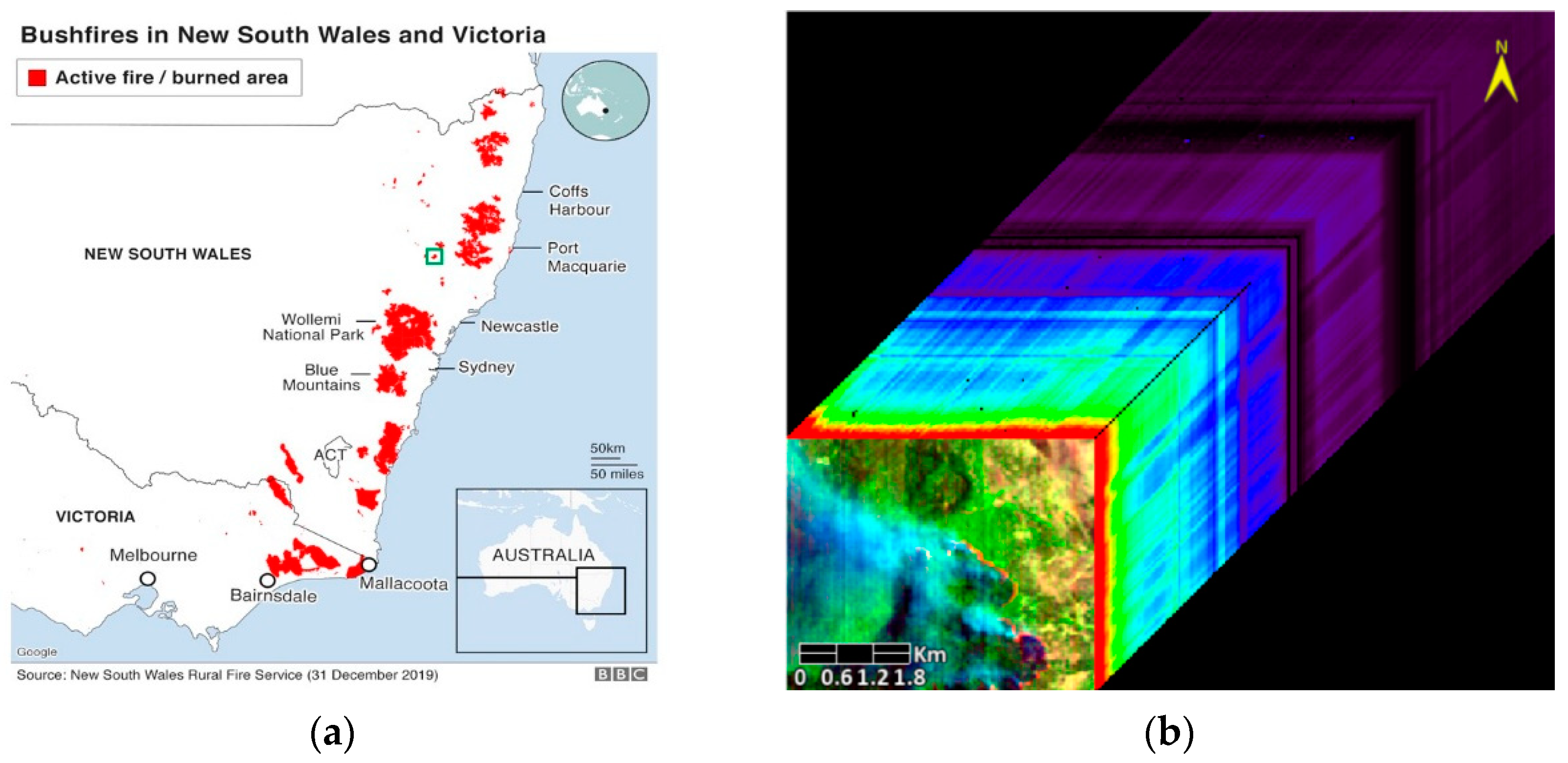
2.1. Case Study

To select the PRISMA hypercube, we searched the PRISMA catalogue [23] for images acquired in the eastern Australian seaboard between October 2019 and February 2020. We then selected the hypercube, acquired on 27 December 2020, in a cloud-free condition. The study was conducted on a subarea (region of interest (ROI)) of the hypercube with a size of 140 × 115 pixels and 212 bands depicting an active fire (Figure 1b) in New South Wales about 250 km north of Sydney in the Ben Halls Gap National Park (BHGNP) which covers 2500 ha, and is situated 60 km south-east of Tamworth and 10 km from the township of Nundle. The park is located at a comparatively high altitude that results in generally cool temperatures and high rainfall. Due to these characteristics, as reported in the BHGNP plan of management [24], wildfires were considered an unusual event at the time that plan was written; however, the simultaneous occurrence of high temperatures and wind speeds and low relative humidity that is required for high-intensity fire behavior, conditions rare for this region, occurred in 2019.

2.2. PRISMA Sensor

The Hyperspectral Precursor of the Application Mission, PRISMA, was launched on 22 March 2019 on board the(Vettore Europeo di Generazione Avanzata) VEGA rocket. The mission has a capacity to acquire up to 223 images per day with a scene of 30 km × 30 km. Generally, the acquisition is based on a priority list and on-demand acquisition request.

The PRISMA imaging payload includes an imaging spectrometer (hyperspectral camera) with VNIR (visible and near-infrared) and SWIR (shortwave infrared) detectors and a panchromatic (PAN) camera detector. The imaging spectrometer provides a continuum of spectral bands spanning between 400 nm and 2500 nm at a ground-sampling distance (GSD) of 30 m/pixel (

Table 1. PRISMA instrument characteristics [27].

Description	Value	Unit
Scene size	30 × 30	Km
Pixel size nadir	30 × 30	M
FOV	2.4	Degrees
Spectral range—VNIR	400–1010	Nm
Spectral range—SWIR	920–2505	Nm
Spectral range—PAN	400–700	Nm
Spectral resolution—VNIR	≤13	Nm
Spectral resolution—SWIR	≤14.5	Nm
Spectral resolution—PAN	≤13.5	Nm
Number of spectral bands—VNIR	66	-
Number of spectral bands—SWIR	174	-
Spatial resolution—VNIR-SWIR	30	m/px
Spatial resolution—PAN	5	m/px
SNR—VNIR	>160 (>450 at 650 nm)	-
SNR—SWIR	>100 (>360 at 1550 nm)	-
SNR—PAN	>240	-
Absolute radiometric accuracy	Better than 5%	-

). The PAN acquires the same area at 5 m/pixel.

The PRISMA hyperspectral instrument differs from previous space-imaging spectrometers because it uses an optical design based on a prism, rather than a grating, to obtain the dispersion of incoming radiation on a 2D focal plane. The advantages of prism-based spectrometers are their compact design and high efficiency [26]; the main disadvantage is the low dispersion [26]. The “instantaneous” spectral and spatial dimensions (across the track) of the PRISMA hyperspectral cube are directly determined by the 2D detectors, while the third dimension (along the track) is determined by the satellite motion (push broom) [27], to provide the 30 × 30 km scene.

2.3. PRISMA Scene

The PRISMA data are made available for free by the Italian Space Agency (ASI) [23,28]. The data are delivered in the HDF5 format with four options: (1) Level 1 (Hyperspectral/PAN) is radiometrically corrected and calibrated TOA (top of atmosphere) data; (2) Level 2B, the Geolocated at Ground Spectral Radiance Product (hyperspectral/PAN); (3) Level 2C, the Geolocated At-surface Reflectance Product (hyperspectral/PAN); and (4) Level 2D, a Geocoded version of the Level 2C product (hyperspectral/PAN). We used the LC1-PRISMA product acquired on 27 December 2019. The image processing was implemented by using the ENVI 5.5 (Harris Geospatial Solution, USA) software and consisted of three steps: (1) applying the scale factor 100 to convert the digital numbers of the L1 product to radiance expressed in Wm⁻²sr⁻¹μm⁻¹ [23,28]; (2) removing noisy bands and building the hyperspectral cube, by stacking the visible and SWIR data; (3) implementing the atmospheric correction and obtaining a reflectance spectrum; (4) producing spectral detection maps and implementing the code (in Matlab 2020b) for the semi-automatic processing of the CO₂-CIBR and HDFI. The hypercube was visually explored to identify the noisy bands affecting the spectra; specifically, the bands within two VNIR spectral intervals (402.2041–426.7687 nm and 972.3630–959.4313 nm) and two SWIR intervals (942.8875–969.7985 nm and 2456.2781–2496.8254 nm) were removed. Because, in our data, the L2 PRISMA reflectance product showed several artifacts in the SWIR that would affect the classification, we preferred to derive the reflectance by applying atmospheric correction to the L1 PRISMA product.

The atmospheric correction was realized by using the QUAC (quick atmospheric correction) available in ENVI 5.5 and applied to the whole PRISMA scene. The QUAC was chosen for several reasons: (a) the image is cloud-free and no cloud shadows are in the scene, and it works best with scenes that contain diverse materials such as soil, vegetation and manmade structures [29], as in our case; (b) the full set of metadata that would be used to implement first-principles radiative-transfer modelling (i.e., fast line-of-sight atmospheric analysis of hypercubes, FLAASH) could not be found in our data; (c) [30] generally found that the results for QUAC were within ±15% of those for FLAASH. The QUAC returns apparent reflectance integer data, with pixel values ranging from 0 to 10,000 (representing 0 to 100% reflectance) [29]. Due to the PRISMA spectral characteristics, the near-shortwave infrared (NIR-SWIR) option available for QUAC was selected, and the pixel values were divided by 10,000 to obtain values spanning between 0 and 1.0 [29]. Figure 2a shows PRISMA single-pixel reflectance spectra corresponding to diverse categories in the imagery.

2.4. Fire Detection Algorithms

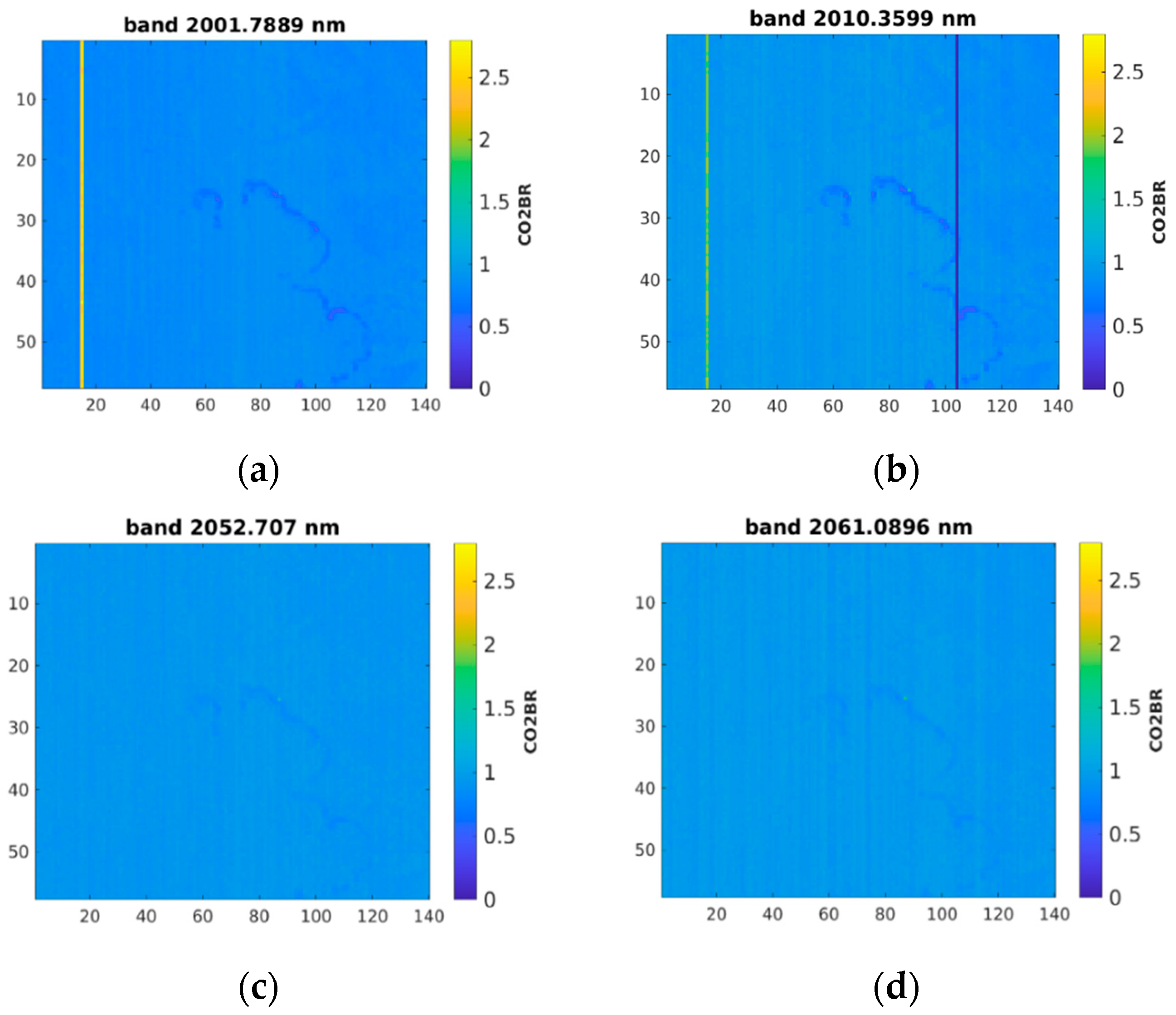
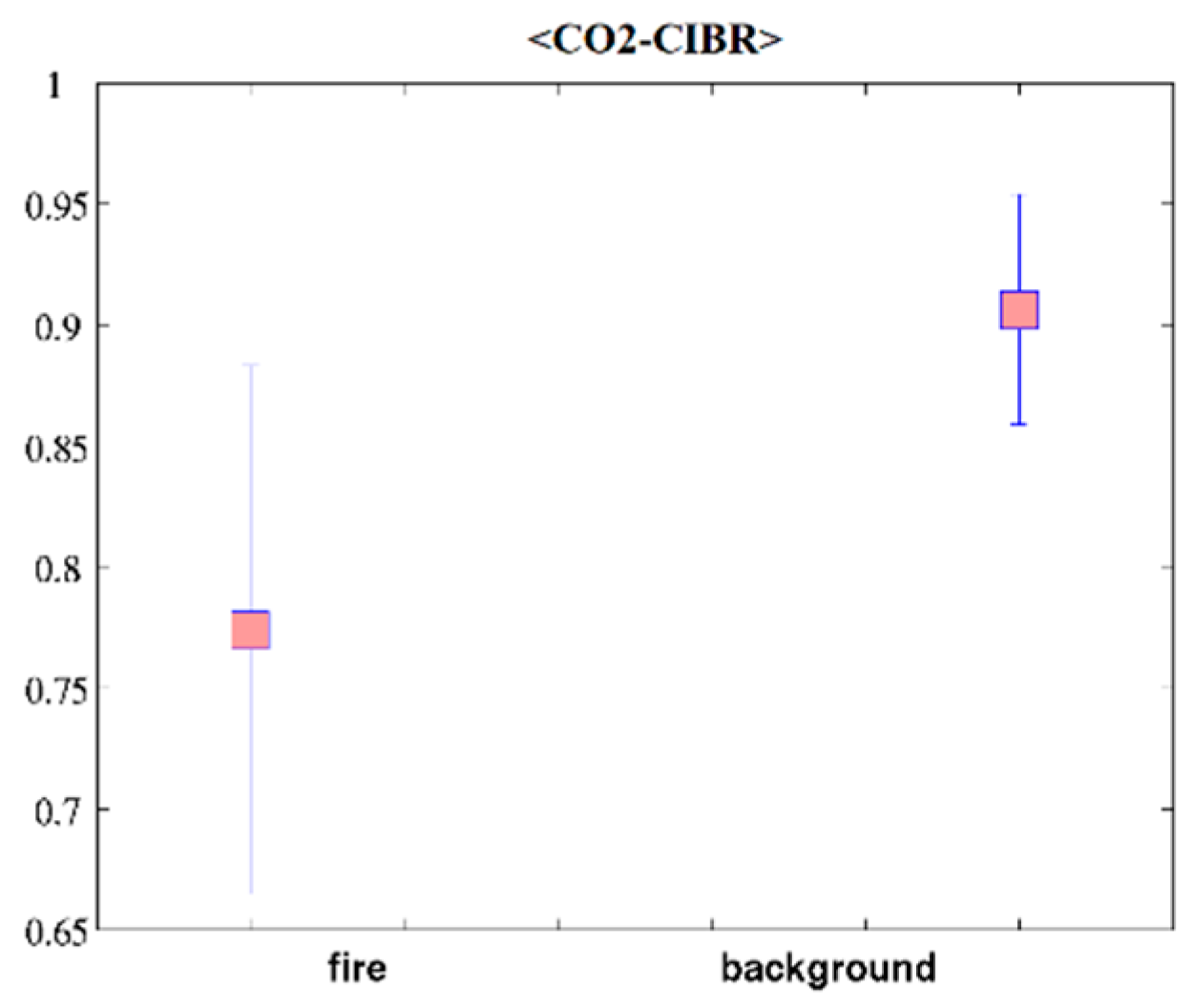
2.4.1. Carbon Dioxide Continuum-Interpolated Band Ratio (CO₂-CIBR)

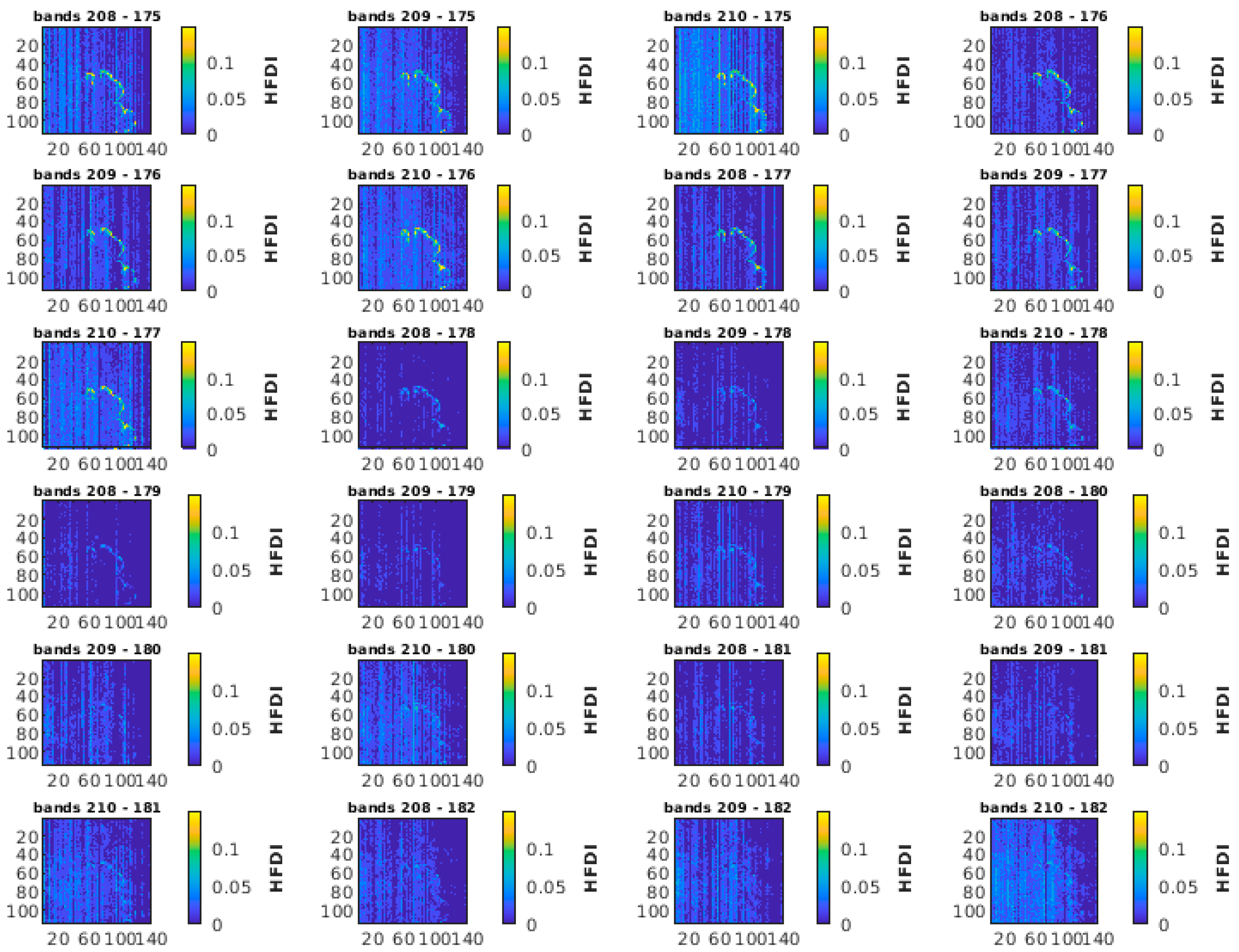
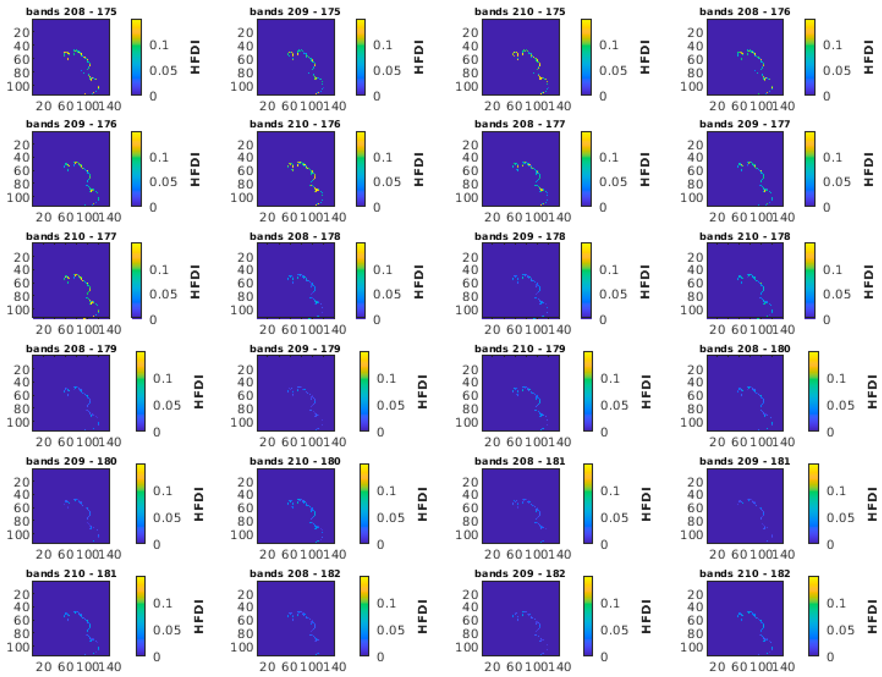
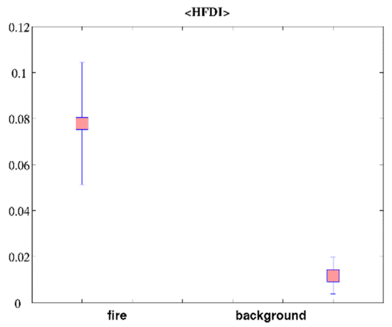
The continuum-interpolated band ratio (CIBR) [2,31] can be used to separate the dominantly emitted radiance from the dominantly reflected radiance and is described by Metric (1).

$$\mathrm{CIBR} =\frac{{\mathrm{L}}_{{\mathsf{\lambda }}_{\mathrm{m}}}}{\begin{array}{c}(\mathrm{w}2\ast {\mathrm{L}}_{{\mathsf{\lambda }}_2}+\mathrm{w}3\ast {\mathrm{L}}_{{\mathsf{\lambda }}_3})\end{array}}$$

(1)

where λ_m is the wavelength at which the absorption is the strongest, λ₂ and λ₃ are the “shoulder” wavelengths with no absorption, and w2 and w3 are weighting factors, where w2 + w3 = 1 and w2 is given by (2).

$$\mathrm{w}2=\frac{({\mathsf{\lambda }}_3 - {\mathsf{\lambda }}_{\mathrm{m}})}{\begin{array}{c}({\mathsf{\lambda }}_3-{\mathsf{\lambda }}_2)\end{array}}$$

(2)

For the carbon dioxide absorption features at 2010 nm were used by [2,6,10] to develop the CO₂-CIBR metric, which turned out to be successful with both airborne (airborne visible/infrared imaging spectrometer, AVIRIS) and EO1-Hyperion data. The PRISMA fire radiance spectra were explored (an example of the spectra is shown in Figure 2b) to select the wavelengths to be used to calculate the CIBRs. The minimum absorption (λ_m) was found for bands centered at 2001.79 nm, 2010.36 nm, 2052.70 nm and 2061.09 nm. For the shoulders, the PRISMA bands centered at 1984.49 nm and 2035.94 nm were selected as λ₂ and λ₃, and those at 2035.94 nm and 2086.04 nm, as λ₂ and λ₃.

The PRISMA central wavelengths and corresponding weighting factors that were used to calculate the CO₂-CIBR are reported in

Table 2. PRISMA wavelengths to be used to derive the diverse CO₂-continuum interpolated band ratio (CIBR)_PRISMA.

λm	λ2	λ3	W2	W3
2001.79	1984.49	2035.94	0.6640	0.3360
2010.36	1984.49	2035.94	0.4972	0.5028
2052.70	2035.94	2086.04	0.66538	0.33462
2061.09	2035.94	2086.04	0.49807	0.50193

.

2.4.2. HFDI

The authors of [6,10] reported fire detection more accurate than that realized with the CIBR by using the hyperspectral fire detection index (HFDI), a normalized difference index defined as

$$\mathrm{HFDI}=\frac{({\mathrm{L}}_{{\mathsf{\lambda }}_1} - {\mathrm{L}}_{{\mathsf{\lambda }}_2})}{\begin{array}{c}({\mathrm{L}}_{{\mathsf{\lambda }}_1}+{\mathrm{L}}_{{\mathsf{\lambda }}_2})\end{array}}$$

(3)

where L_λ1 and L_λ2 are the spectral radiances at two SWIR bands around 2430 nm and 2060 nm expressed in Wm⁻²sr⁻¹μm⁻¹. These two bands provided better performance when using AVIRIS spectral data [6]. In addition, [10] highlighted that this metric needs to be adapted to the sensor noise level around the spectral range 2400–2500 nm. Because the PRISMA sensor is very new and its derived products are under continuous evaluation, we derived the HFDI for a series of band combinations following an approach similar to that used by [10] for EO1-Hyperion to identify the best combination.

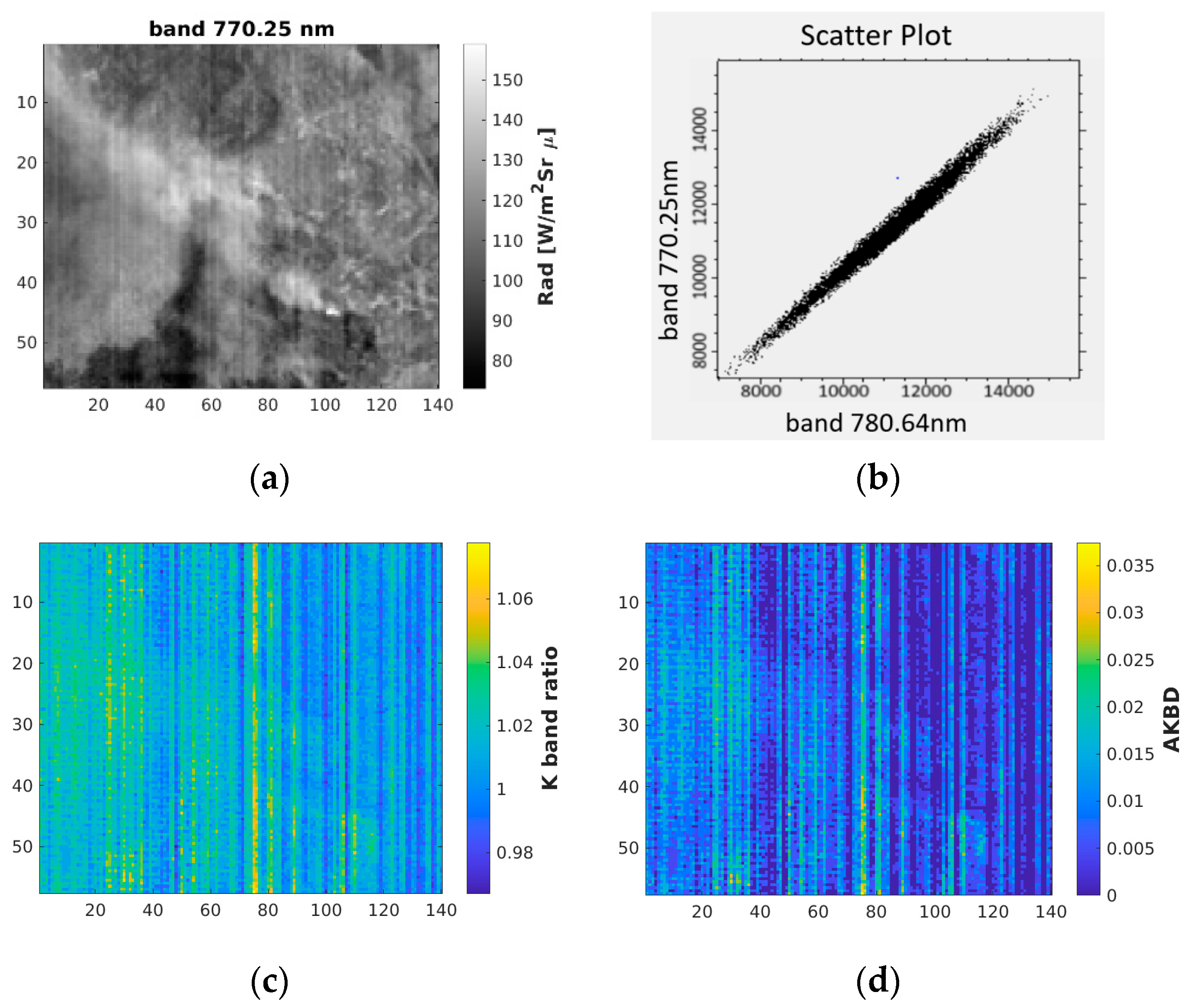
2.4.3. Potassium Emission

Trace elements such as potassium, sodium and phosphorus [32,33,34] present in the biomass ionized at flaming temperatures emit signals at specific wavelengths that can be detected in the spectrum measured by a spectrometer [5,7,10]. These signals have been used to locate wildfire flaming phases using laboratory and airborne sensors [5,7]; their ability to be used to detect flaming from space [2,5,10] depending on a range of factors warrants further exploration [10]. Because the K emission lines occur at two specific wavelengths (766.5 nm and 769.9 nm) [7], two metrics were developed: (1) the K emission index [6,10], defined by the ratio of the radiances measured at the K emission wavelength (770 nm) and at the proximal band (780 nm), not influenced by the emission and acting as the background; (2) the AKBD metric, a normalized difference between the K emission bands and the background bands [5,10].

2.5. Fire Reference for Comparison

In order to compare the detection performance of the metrics, the fire pixels need to be discriminated from non-fire pixels. To do this, we applied a supervised classification to the reflectance PRISMA scene, to select endmembers (the truth to be used to train the classification algorithm). Specifically, we selected 48 pixels representing smoke, 48 pixels for the bare soil class (bare soil/road/anthropic), 36 pixels for vegetation (high vegetation, bushes and low vegetation), 12 pixels for freshly burned areas, and 48 pixels for active fires. Of the ground truth, 83% was used for the training, while the remaining 17% was selected for the classification validation. The pixels were selected by exploring the false color composite (Figure 1b) and looking at the PRISMA spectral profile, which was comparable with the corresponding classes that can be found in the literature [10,35]. In addition, pan sharpening was attempted to fuse a panchromatic-camera, 5 m-resolution PRISMA product and L2C PRISMA (VNIR-SWIR) projected product to obtain higher-resolution images, to be used for fire pixel validation. The data were fused using the Gram–Schmidt pan sharpening function available in ENVI 5.5, and although the L2D data were relatively noisy, they were used to visually confirm the burning areas. The classification was implemented by using the support vector machine (SVM) [36,37]. The SVM is considered, along with the random forest classifier and artificial neural networks, one of the most effective supervised classification methods [38] for multidimensional, large-scale image data. The SVM method algorithms perform well on noisy data and small numbers of training pixels [38,39], are suitable for anomaly detection [40] and are usually more accurate than other classification algorithms [37,41].

The kernel type was set as polynomial, with the value set to 2 and the penalty parameter set to 200. The result is showed in Figure 3b.

The overall classification accuracy was 96.87%, with a K coefficient of 0.96. The class fire, which is was of interest in this study, resulted in commission (false positive) and omission (false negative) error of 0%).

Determining if there was good agreement with the other classes regarding this result was beyond the scope of this study. The classification was used to create a mask, with values equal to 1 corresponding to fire pixels and those equal to 0, the background (not burning pixels), for use in assessing the performance of the detection indices.

3. Results

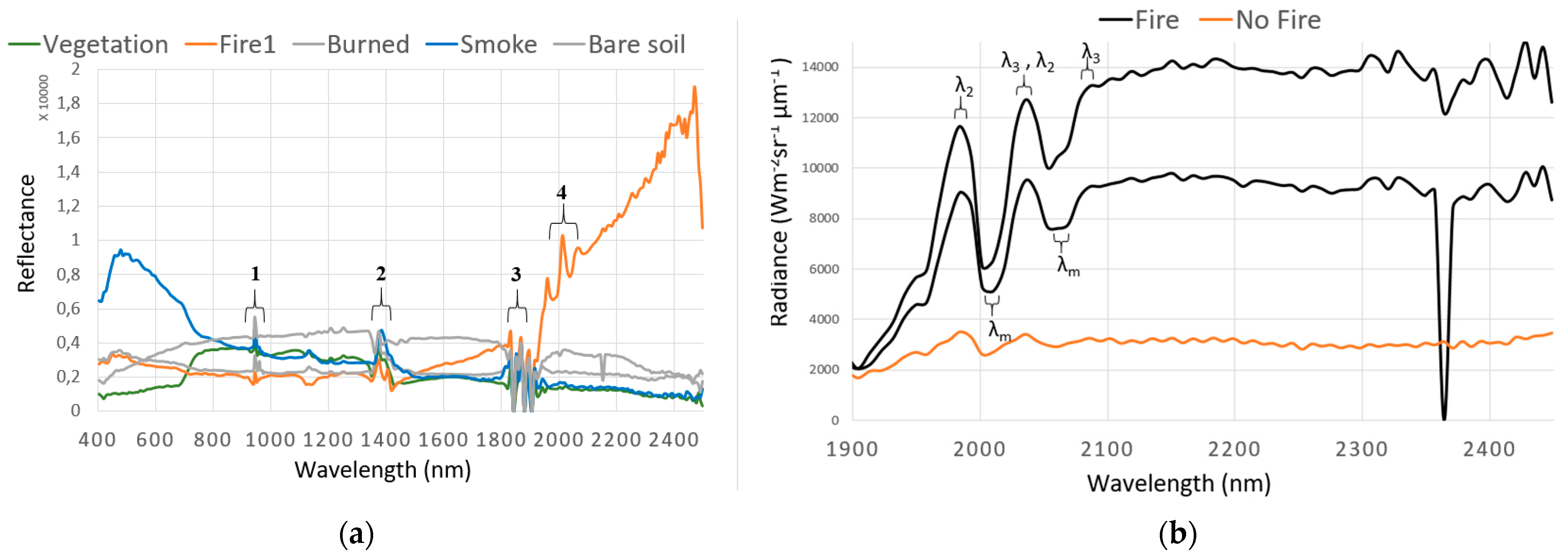
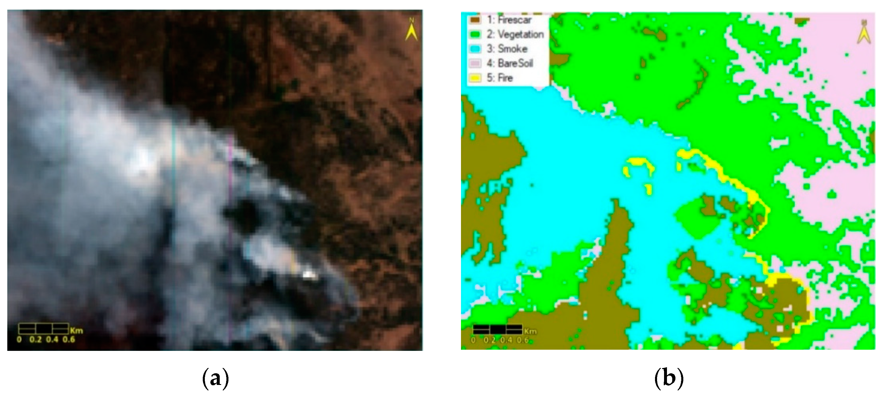
Fire Detection Analysis

The fire localization analysis was conducted for the three fire detection indices adapted to the PRISMA band features.

The detection rate was calculated by linear regression between the fire pixels derived by the specific indices and the ones resulting from the reference (the SVM-derived fire mask). A thresholding approach was used to identify the detected fire pixels. The cut-off ranges were obtained by automatically computing the minimum and maximum values for each index considering only pixels inside the “fire” class. (1) The cut-off minimum was obtained by subtracting two standard deviations (2σ) from the mean, and (2) the cut-off maximum, by adding one standard deviation (1σ) to the mean. The cut-off intervals were used to discriminate fire from background for each index frame.

The first index to be analyzed was the CO₂-CIBR. Figure 4 shows the CO₂-CIBR maps for the four band combinations. We can observe that, despite the striping noise, the front fire is recognizable. Specifically, it was better delineated when the absorption bands centered at 2001.79 nm and 2010.36 nm were used.

Table 3. CO₂-CIBR detection rate.

Band 1	Band 2	Band 3	λm (nm)	λ2 (nm)	λ3 (nm)	Cut-off Min	Cut-off Max	Detection Rate
169	167	173	2001.79	1984.49	2035.94	0.55094	0.74674	0.81598
179	167	173	2010.36	1984.49	2035.94	0.32421	0.85531	0.29205
175	173	179	2052.71	2035.94	2086.04	0.78086	0.89774	0.25083
176	173	179	2061.09	2035.94	2086.04	0.75938	0.93708	0.13561

shows the results obtained in terms of the detection rate. A detection rate of 0.81 and a cut-off ranging between 0.550 and 0.74674 were determined for the CO₂-CIBR having the minimum absorption band centered at 2001.36 nm, in agreement with the visual interpretation in Figure 4a.

Instead detection rate of 0.29 was obtained for the CO₂-CIBR centered at 2010.36 nm very low compared to what was suggested by visual interpretation.

A low detection rate, consistent with the visual interpretation, was obtained for the other two CO₂-CIBRs (Figure 4c,d). In these cases, the striping noise was relatively uniformly distributed and comparable with the signal.

To mitigate the effect of the noise on the single bands [10], the mean value of the CO₂-CIBR indices was calculated. The result (Figure 5) provides a cut-off of 0.7741 ± 0.1091, well separated from the mean background value (Figure 5).

The HFDI was retrieved by applying Equation (2) for the 24 possible band combinations (Figure 6).

Table 4. This table reports the PRISMA bands and corresponding wavelengths used to derive the HFDI, the used cut-off and the detection rate.

Band 1	Band 2	Central λ1 (nm)	Central λ2 (nm)	Cut-Off Min	Cut-Off Max	Detection Rate
208	175	2312.80	2052.70	0.08	0.19192	0.8223
209	175	2320.58	2052.71	0.08	0.19111	0.75852
210	175	2327.54	2052.72	0.08	0.21888	0.83235
208	176	2312.85	2061.08	0.05	0.17544	0.88431
209	176	2320.59	2061.09	0.08	0.17544	0.67228
210	176	2327.55	2061.10	0.08	0.20339	0.84063
208	177	2312.86	2069.49	0.05	0.16256	0.79732
209	177	2320.60	2069.50	0.05	0.15021	0.83295
210	177	2327.56	2069.51	0.08	0.17842	0.76144
208	178	2312.87	2077.70	0.05	0.092593	0.50731
209	178	2320.61	2077.71	0.05	0.080645	0.36171
210	178	2327.57	2077.72	0.05	0.10938	0.64754
208	179	2312.88	2086.04	0.05	0.075472	NaN 1
209	179	2320.62	2086.05	0.05	0.059289	NaN
210	179	2327.58	2086.06	0.05	0.088123	NaN
208	180	2312.89	2094.36	0.05	0.066667	NaN
209	180	2320.63	2094.37	0.05	0.058824	NaN
210	180	2327.59	2094.38	0.05	0.083969	NaN
208	181	2312.90	2102.49	0.05	0.065421	NaN
209	181	2320.64	2102.50	0.05	0.050000	NaN
210	181	2320.59	2102.51	0.05	0.073684	NaN
208	182	2327.55	2110.77	0.05	0.064516	NaN
209	182	2312.86	2110.78	0.05	0.058824	NaN
210	182	2320.60	2110.79	0.05	0.076923	NaN

¹ NaN (not a number).

reports the cut-off ranges and detection rates obtained for the 24 band combinations.

In this case, a bias value of 0.05 or 0.08 (Table 4) was added to the cut-off min in order to discriminate the “fire” from background. The results of the linear regression in terms of the detection rate are reported in Table 4. We can observe that nine HFDIs out of the 24 resulted in detection rates better than 0.76. The best performance was obtained by using the bands 2312.85 nm and 2061.08 nm, with a detection rate of 0.88. Twelve detection rates resulted in a “not a number” output.

To highlight the fire front, a mask was applied to the background (Figure 7).

The mean value of the HFDIs was calculated. The result provides a cut-off of 0.0778 ± 0.0265, well separated from the mean background value (Figure 8).

Finally, we calculated the potassium emission index by using the PRISMA band 44, centered at 770.25 nm (for the emission, Figure 9a) and the band 45 centered at 780.63 nm (for the background). The scatter plot obtained for the two bands shows a high correlation between the bands (Figure 9b). The results for the two indices are shown in Figure 9c,d. We can observe the prevalence of the striping effect over the signal. The fire is not recognizable when using the band ratio, and it is blurred and difficult to delineate when using the AKBD metric.

4. Discussion

We analyzed the three fire detection indices based on daytime acquisition by the new PRISMA sensor over the bushfires that occurred in Ben Halls Gap National Park in 2019. In our PRISMA subscene, both the CO₂-CIBR and HFDI indices were able to discriminate the fire front. Regarding the CO₂-CIBR, the best performance was obtained by using the band centered at 2001.79 nm (absorption) and those at 1984.49 nm and 2035.94 nm (the “shoulders”). However, when we look at the CO₂-CIBR calculated with the PRISMA bands (2010.36 nm, 1984.49 nm and 2035.94 nm) very close to the AVIRIS [10] ones (2010 nm, 1990 nm and 2040 nm), the obtained map (Figure 4b) and the detection rate (Table 3) look very different. The lower detection rate is due to the presence of a stripe whose values are comparable to those of fire. This needs to be further investigated in a range of PRISMA scenes.

The higher detection rate of the PRISMA CO₂-CIBR with a band combination (2001.79 nm, 1984.49 nm and 2035.94 nm) comparable to that (1981.86 nm, 2032.35 nm 2002.06 nm) used by [10] for the CO₂-CIBR for EO1-Hyperion is interesting found.

The results obtained with the HFDI agree with the literature [10], which indicates that the HFDI should perform better than the CO₂-CIBR. The best band combination turned out to be 2312.85 nm and 2061.08 nm, resulting in a detection rate of 0.88; this is very close to the AVIRIS one (2430 nm and 2061 nm) reported in [10]. When comparing the best-performing EO1-Hyperion combinations used in [10] with the “almost” corresponding PRISMA combination, we obtained NaN. In Table 4, it is possible to observe how the cut-off ranges for these combinations are too narrow to permit a distinction between fire and background. Even looking at the single HFDI images in Figure 6, it is evident that, from the thirteenth combination onward, the front of the fire blends into the background.

The potassium (K)-emission-based index underperformed compared to the other two indices. Diverse aspects need to be considered to interpret this result. The full width half maximum (FWHM) of PRISMA in the used bands is 12.7 nm, so the separation is challenged compared to that for the ≤10 nm FWHM of EO1-Hyperion or AVIRIS [10]. Another effect to take into account is the striping effect present in our data that affects each band in a different way. This effect is stronger or weaker depending on the signal present in the image. For example, in an absorption band, all the signal is absorbed and the striping is imaged. The K emission band is very close to the O₂ absorption band centered at 765 nm, and it can be weakened by the two combined effects. Furthermore, the type of combustion (i.e., crown) as well as the vegetation type can contribute, as diverse vegetation species contain various amounts of K [33]. Finally, the presence of smoke can attenuate the signal [10] as well as the spatial resolution (30 m/px) [9] if only a fraction of the pixel is flaming.

In agreement with the literature for the EO1-Hyperion, our first results show that the HFDI performs better, in terms of fire detection, than the CO₂-CIBR and AKBD. This is promising considering the difference in spectral resolution between PRISMA (~13 nm) and EO1-Hyperion (10 nm).

Future efforts should focus on the analysis of fires in diverse ecosystems (present in the scene or found in other PRISMA data), to determine if a common threshold can be found for retrieving the HFDI.

5. Conclusions

This study concerns a multimethod analysis for studying active land fires in New South West Australia that occurred during the 2019 bushfire season using hyperspectral techniques from space. We report the first case study of active fire characterization by using data from the new PRISMA space mission by the Italian Space Agency. The fire occurred in the Ben Halls Gap National Park during the bushfire season of 2019/2020 in Australia and was imaged by the PRISMA sensor. Firstly, we wanted to verify the ability of the PRISMA sensor to provide spectral features useful for characterizing phenomena, such as wildfires, different from those considered in its primary mission objectives; secondly, we tested three fire detection indices that relate the measured radiance to the intrinsic characteristics of the phenomena, such as the ionization of trace elements (AKBD index), carbon dioxide emissions (the CO₂-CIBR index) and radiance values in the SWIR bands (HFDI).

The indices were adapted to PRISMA spectral features. Atmospheric correction was implemented to transform radiance into reflectance; a supervised classification, using the SVM approach, was used to retrieve the detection rate.

The obtained reflectance spectra are representative of diverse classes present in the scene. The overall performance of the instrument in terms of the radiance in our data was good. However, the presence of the striping effect can influence the performance of the indices.

In terms of the detection performance, the results agree with the literature to date [10]. In addition, PRISMA resulted in improved CO₂-CIBR and HFDI performance compared to the EO1-Hyperion satellite [10].

The AKBD data resulted in underperformance. This is possibly due to multiple factors including the spectral resolution in the potassium band (12 nm), the striping noise, attenuation from the atmosphere and the spatial resolution.

The results are promising in terms of using PRISMA for active fire characterization using SWIR bands.

To close, it is relevant to mention that, due to the complexity of the hyperspectral sensors and the large number of data they collects, there is a gap between case studies and operational applications. In this context, synergies between future missions (i.e., EnMap, Chime, Surface Biology and Geology -SBG and Spaceborne Hyperspectral Applicative Land and Ocean Mission-SHALOM) and knowledge sharing will be very important for providing complementary information.

References

1. Kaufman, Y.J.; Justice, C.O.; Flynn, L.P.; Kendall, J.D.; Prins, E.M.; Giglio, L.; Ward, D.E.; Menzel, W.P.; Setzer, A.W. Potential global fire monitoring from EOS-MODIS. J. Geophys. Res. Space Phys. 1998, 103, 215–238. [Google Scholar] [CrossRef]
2. Dennison, P.E. Fire detection in imaging spectrometer data using atmospheric carbon dioxide absorption. Int. J. Remote Sens. 2006, 27, 3049–3055. [Google Scholar] [CrossRef]
3. Flannigan, M.D.; Haar, T.H.V. Forest fire monitoring using NOAA satellite AVHRR. Can. J. For. Res. 1986, 16, 975–982. [Google Scholar] [CrossRef]
4. Veraverbeke, S.; Dennison, P.; Gitas, I.; Hulley, G.; Kalashnikova, O.; Katagis, T.; Kuai, L.; Meng, R.; Roberts, D.; Stavros, N. Hyperspectral remote sensing of fire: State-of-the-art and future perspectives. Remote Sens. Environ. 2018, 216, 105–121. [Google Scholar]
5. Amici, S.; Wooster, M.J.; Piscini, A. Multi-resolution spectral analysis of wildfire potassium emission signatures using laboratory, airborne and spaceborne remote sensing. Remote Sens. Environ. 2011, 115, 1811–1823. [Google Scholar] [CrossRef]
6. Dennison, P.E.; Roberts, D.A. Daytime fire detection using airborne hyperspectral data. Remote Sens. Environ. 2009, 113, 1646–1657. [Google Scholar] [CrossRef]
7. Vodacek, A.; Kremens, R.L.; Fordham, A.J.; VanGorden, S.C.; Luisi, D.; Schott, J.R.; Latham, D.J. Remote optical detection of biomass burning using a potassium emission signature. Int. J. Remote Sens. 2002, 23, 2721–2726. [Google Scholar] [CrossRef]
8. Dennison, P.E.; Matheson, D.S. Comparison of fire temperature and fractional area modeled from SWIR, MIR, and TIR multispectral and SWIR hyperspectral airborne data. Remote Sens. Environ. 2011, 115, 876–886. [Google Scholar] [CrossRef]
9. Matheson, D.S.; Dennison, P.E. Evaluating the effects of spatial resolution on hyperspectral fire detection and temperature retrieval. Remote Sens. Environ. 2012, 124, 780–792. [Google Scholar] [CrossRef]
10. Waigl, C.F.; Prakash, A.; Stuefer, M.; Verbyl, D.; Dennison, P. Fire detection and temperature retrieval using EO-1 Hyperion data over selected Alaskan boreal forest fires. Int. J. Appl. Earth Obs. Geoinf. 2019, 81, 72–84. [Google Scholar] [CrossRef]
11. Guanter, L.; Kaufmann, H.; Segl, K.; Foerster, S.; Rogass, C.; Chabrillat, S.; Kuester, T.; Hollstein, A.; Rossner, G.; Chlebek, C.; et al. The EnMAP Spaceborne Imaging Spectroscopy Mission for Earth Observation. Remote Sens. 2015, 7, 8830–8857. [Google Scholar] [CrossRef] [Green Version]
12. Nieke, J.; Rast, M. Towards the Copernicus Hyperspectral Imaging Mission For The Environment (CHIME). In Proceedings of the IGARSS 2018–2018 IEEE International Geoscience and Remote Sensing Symposium, Valencia, Spain, 22–27 July 2018; pp. 157–159. [Google Scholar] [CrossRef]
13. Pitman, A.J.; Narisma, G.T.; McAneney, J. The impact of climate change on the risk of forest and grassland fires in Australia. Clim. Chang. 2007, 84, 383–401. [Google Scholar] [CrossRef]
14. Kumar, S.V.; Holmes, T.; Andela, N.; Dharssi, I.; Hain, C.; Peters-Lidard, C.; Mahanama, S.P.; Arsenault, K.R.; Nie, W.; Getirana, A. The 2019–2020 Australian drought and bushfires altered the partitioning of hydrological fluxes. Geophys. Res. Lett. 2021, 48, e2020GL091411. [Google Scholar] [CrossRef]
15. Weber, D.; Moskwa, E.; Robinson, G.; Bardsley, D.; Arnold, J.; Davenport, M. Are we ready for bushfire? Perceptions of residents, landowners and fire authorities on Lower Eyre Peninsula, South Australia. Geoforum 2019, 107, 99–112. [Google Scholar] [CrossRef]
16. Deb, P.; Moradkhani, H.; Abbaszadeh, P.; Kiem, A.S.; Engström, J.; Keellings, D.; Sharma, A. Causes of the Widespread 2019–2020 Australian Bushfire Season. Earths Futur. 2020, 8. [Google Scholar] [CrossRef]
17. Oloruntoba, R. Plans never go according to plan: An empirical analysis of challenges to plans during the 2009 Victoria bushfires. Technol. Forecast. Soc. Chang. 2013, 80, 1674–1702. [Google Scholar] [CrossRef]
18. King, A.D.; Pitman, A.J.; Henley, B.J.; Ukkola, A.M.; Brown, J.R. The role of climate variability in Australian drought. Nat. Clim. Chang. 2020, 10, 177–179. [Google Scholar] [CrossRef]
19. McArthur, A.G. Fire Behaviour in Eucalypt Forests. Forestry and Timber Bureau, Canberra. 1967. Available online: https://catalogue.nla.gov.au/Record/2275488 (accessed on 3 March 2021).
20. Australia in December 2019; Australian Government Bureau of Meteorology. Available online: http://www.bom.gov.au/climate/current/month/aus/archive/201912.summary.shtml (accessed on 30 March 2021).
21. Fire and the Environment 2019-20 Summary; Department of Planning, Industry and Environment: Parramatta, Australia, 2020; ISBN 978-1-922318-57-2. Available online: https://www.environment.nsw.gov.au/research-and-publications/publications-search/fire-and-the-environment-2019-20-summary (accessed on 27 October 2020).
22. NSW Rural Fire Service. Available online: http://www.rfs.nsw.gov.au/news-and-media/media-releases/dangerous-fire-conditions-extreme-fire-danger (accessed on 27 October 2020).
23. PRISMA Catalogue Web. Available online: www.prisma.asi.it (accessed on 1 December 2020).
24. Ben Halls Gap National Park Plan of Management. Available online: https://www.environment.nsw.gov.au/-/media/OEH/Corporate-Site/Documents/Parks-reserves-and-protected-areas/Parks-plans-of-management/ben-halls-gap-national-park-plan-of-management-020091.pdf (accessed on 27 October 2020).
25. BBC News. Available online: https://ichef.bbci.co.uk/news/320/cpsprodpb/0677/production/_110355610_nsw_vtr_fires_dec31_976-nc.png (accessed on 10 December 2020).
26. Smith, R.C. Astrophysical Techniques, Sixth Edition, by C.R. Kitchin. Contemp. Phys. 2014, 55, 359–360. [Google Scholar] [CrossRef]
27. Coppo, P.; Brandani, F.; Faraci, M.; Sarti, F.; Cosi, M. Leonardo Spaceborne Infrared Payloads for Earth Observation: SLSTRs for Copernicus Sentinel 3 and PRISMA Hyperspectral Camera for PRISMA Satellite. In Proceedings of the 15th International Workshop on Advanced Infrared Technology and Applications (AITA 2019), Florence, Italy, 17–19 September 2019; Volume 27, p. 1. [Google Scholar] [CrossRef] [Green Version]
28. Guarini, R.; Loizzo, R.; Facchinetti, C.; Longo, F.; Ponticelli, B.; Faraci, M.; Dami, M.; Cosi, M.; Amoruso, L.; De Pasquale, V.; et al. PRISMA hyperspectral mission products. In Proceedings of the IGARSS 2018–2018 IEEE International Geoscience and Remote Sensing Symposium, Valencia, Spain, 22–27 July 2018; pp. 179–182. [Google Scholar] [CrossRef]
29. Quick Atmospheric Correction (QUAC). Available online: https://www.l3harrisgeospatial.com/docs/quac.html (accessed on 15 December 2020).
30. Bernstein, L.S.; Jin, X.; Gregor, B.; Adler-Golden, S.M. The Quick Atmospheric Correction (QUAC) Code: Algorithm Description and Recent Upgrades. SPIE Opt. Eng. 2012, 51, 111719. [Google Scholar] [CrossRef]
31. Gao, B.-C.; Goetz, A.F.H. Determination of Total Column Water Vapor in the Atmosphere at High Spatial Resolution from AVIRIS Data Using Spectral Curve Fitting and Band Ratioing Techniques. In Imaging Spectroscopy of the Terrestrial Environment; SPIE: Bellingham, WA, USA, 1990; Volume 1298, pp. 138–149. [Google Scholar]
32. Hartley, T.N. Increasing the Potassium Use Efficiency of Crops. Doctoral Dissertation, University of York, York, UK, September 2017. Available online: http://etheses.whiterose.ac.uk/20019/ (accessed on 3 March 2021).
33. Clery, D.S.; Mason, P.E.; Rayner, C.M.; Jones, J.M. The effects of an additive on the release of potassium in biomass combustion. Fuel 2018, 214, 647–655. [Google Scholar] [CrossRef]
34. Díaz-Ramírez, M.; Frandsen, F.J.; Glarborg, P.; Sebastián, F.; Royo, J. Partitioning of K, Cl, S and P during combustion of poplar and brassica energy crops. Fuel 2014, 134, 209–219. [Google Scholar] [CrossRef]
35. McMorrow, J.N.; Coe, H.; McFiggans, G.; Dold, J.; Tantanasi, I.; Gareth, C.; Aylen, J.; Millin-Chalabi, G.; Agnew, C.; Amici, S. Wildfires@Manchester, Poster Royal Society. 2015. Available online: http://www.kfwf.org.uk/_assets/documents/RoySoc_FirePoster_UnivOf_Manchester_McMorrow_etal_5oct15.pdf (accessed on 10 December 2020).
36. Hsu, C.-W.; Chang, C.-C.; Lin, C.-J. A Practical Guide to Support Vector Classification. 2010. Available online: http://www.csie.ntu.edu.tw/~cjlin/papers/guide/guide.pdf (accessed on 5 October 2015).
37. Foody, G.M.; Mathur, A. A Relative Evaluation of Multiclass Image Classification by Support Vector Machines. IEEE Trans. Geosci. Remote Sens. 2004, 42, 1335–1343. [Google Scholar] [CrossRef] [Green Version]
38. Sabat-Tomala, A.; Raczko, E.; Zagajewski, B. Comparison of Support Vector Machine and Random Forest Algorithms for Invasive and Expansive Species Classification Using Airborne Hyperspectral Data. Remote Sens. 2020, 12, 516. [Google Scholar] [CrossRef] [Green Version]
39. Ghosh, A.; Fassnacht, F.E.; Joshi, P.K.; Koch, B. A framework for mapping tree species combining hyperspectral and LiDAR data: Role of selected classifiers and sensor across three spatial scales. Int. J. Appl. Earth Obs. Geoinf. 2014, 26, 49–63. [Google Scholar] [CrossRef]
40. Xiang, P.; Zhou, H.; Li, H.; Song, S.; Tan, W.; Song, J.; Gu, L. Hyperspectral anomaly detection by local joint subspace process and support vector machine. Int. J. Remote Sens. 2020, 41, 3798–3819. [Google Scholar] [CrossRef]
41. Amici, S.; Piscini, A.; Buongiorno, M.; Pieri, D. Geological classification of Volcano Teide by hyperspectral and multispectral satellite data. Int. J. Remote Sens. 2012, 34, 3356–3375. [Google Scholar] [CrossRef]
Figure 1. (a) Active fire/burned area map [25] for bushfires in New South Wales and Victoria on 31 December 2019. The green square in the map corresponds to Precursore IperSpettrale della Missione Applicativa (PRISMA) imaged area; (b) PRISMA subarea hypercube acquired on 27 December 2019. Red, Green, Blue (RGB), false color band composition with central wavelengths located at 1646.9205 nm, 8,548,984 nm and 579.1278 nm shows a derived fire front extension of about 5 km.
Remotesensing 13 01410 g001
Figure 2. (a) PRISMA reflectance spectra corresponding to five categories: vegetation, fire, smoke, bare soil and freshly burned. The black bracket number 1 indicates very near-shortwave infrared (VNIR-SWIR) bands overlapping; the brackets number 2 and 3 indicate atmospheric attenuation from water vapor that can occur at 1400 nm and 1900 nm respectively; the bracket number 4 indicates the CO2 absorption bands around 2000 nm. (b) Two PRISMA fire radiance spectra against the background (no fire) radiance show absorption bands around 2000 nm and 2010 nm (λm) and around 2050 nm and 2060 nm (λm), where CO2 absorption bands are expected. The positions of the wavelength corresponding to the “shoulders” are indicated as λ2 (shoulder at the left of λm) and λ3 (shoulder at the right of λm), respectively.
Remotesensing 13 01410 g002
Figure 3. (a) RGB visible composition of PRISMA region of interest shows a dense fire smoke originating from diverse locations; (b) classification result corresponding to the selected region of interest (ROI) by using the complete VNIR–SWIR PRISMA spectral range. The yellow pixels correspond to active fire; light blue corresponds to the smoke class; brown, to freshly burned; green is the vegetation; and light pink, bare soil.
Remotesensing 13 01410 g003
Figure 4. CO2-continuum interpolated band ratio (CIBR) maps. (a) CO2-CIBR derived for minimum absorption band centered at 2001.79 nm; (b) CO2-CIBR derived for minimum absorption band centered at 2010.36 nm; (c) CO2-CIBR derived for minimum absorption band centered at 2052.71 nm; (d) CO2-CIBR derived for minimum absorption band centered at 2061.09 nm.
Remotesensing 13 01410 g004
Figure 5. Separability of Ben Halls Gap National Park fire indices; mean value of the four CO2-CIBRs is 0.7741 ± 0.1091, and mean value of the background is 0.9664 ± 0.0477.
Remotesensing 13 01410 g005
Figure 6. Hyperspectral fire detection index (HFDI) maps for the twenty-four combinations.
Remotesensing 13 01410 g006
Figure 7. HFDI maps for all twenty-four combinations masked by support vector machine (SVM) classification to evidence fire front.
Remotesensing 13 01410 g007
Figure 8. Separability of Ben Halls Gap National Park fire indices HFDI mean value over the twenty-four combinations is 0.0778 ± 0.0265, and the background is 0.0117 ± 0.0080.
Remotesensing 13 01410 g008
Figure 9. (a) Gray color PRISMA imagery at 770.25 nm; (b) scatter plot for PRISMA bands at 770.25 nm vs. 780.64 nm, showing high correlation between band where potassium emission is expected and that for the background; (c) potassium emission band ratio; (d) advance K band difference (AKBD) normalized index map.
Remotesensing 13 01410 g009