Abstract
Three-dimensional (3D) building models play an important role in digital cities and have numerous potential applications in environmental studies. In recent years, the photogrammetric point clouds obtained by aerial oblique images have become a major source of data for 3D building reconstruction. Aiming at reconstructing a 3D building model at Level of Detail (LoD) 2 and even LoD3 with preferred geometry accuracy and affordable computation expense, in this paper, we propose a novel method for the efficient reconstruction of building models from the photogrammetric point clouds which combines the rule-based and the hypothesis-based method using a two-stage topological recovery process. Given the point clouds of a single building, planar primitives and their corresponding boundaries are extracted and regularized to obtain abstracted building counters. In the first stage, we take advantage of the regularity and adjacency of the building counters to recover parts of the topological relationships between different primitives. Three constraints, namely pairwise constraint, triplet constraint, and nearby constraint, are utilized to form an initial reconstruction with candidate faces in ambiguous areas. In the second stage, the topologies in ambiguous areas are removed and reconstructed by solving an integer linear optimization problem based on the initial constraints while considering data fitting degree. Experiments using real datasets reveal that compared with state-of-the-art methods, the proposed method can efficiently reconstruct 3D building models in seconds with the geometry accuracy in decimeter level.
1. Introduction
Three-dimensional (3D) building models play an important role in constructing digital cities and have numerous environmental applications in areas such as urban planning [1], smart city [2], environmental analysis [3], and other civil engineering [4]. In recent years, with the rapid development of aerial vehicles, cameras, and image-processing technologies, aerial oblique images have become a major data source for 3D city modeling [5,6]. Due to the time-consuming and labor-intensive nature of manual modeling processes, researchers in the photogrammetry, computer vision, and graphic communities have developed automatic building model reconstruction methods [7,8,9,10]. Due to the presence of occlusions in complex city scenes and noise in forward-intersecting point clouds, some building features (e.g., planes, edges) are degraded or even missed in the collected point clouds, which leads to unreliable recovery of the topological relationships [11].
To address this problem, various data- and model-driven methods (or their combination) have been proposed in recent years and substantial improvements in quality have been achieved [9,12,13,14]. However, for complex buildings with imperfect point coverage, it is difficult to automatically and efficiently reconstruct building models with desired Level of Detail (LoD) [15,16], hindering environmental simulation, spatial analysis, and other model-based applications. To solve this problem, in this paper, a novel framework which combines the rule-based and the hypothesis-based method is proposed for the efficient reconstruction of high-quality polygonal building models. Starting with the point clouds of a single building, the planar primitives and corresponding boundaries are extracted and regularized to obtain abstracted building counters, followed by a two-stage reconstruction. In the first stage, the regularity and adjacency of the building counters are used to recover the topological relationship between different primitives and produce an initial reconstruction. In the second stage, the topologies of ambiguous areas are removed and reconstructed by solving an integer linear optimization problem based on the initial reconstruction.
The major contributions of this paper are as follows:
- (1)
- A novel framework for 3D building reconstruction which combines the efficiency of traditional rule-based methods and the integrity of recently developed hypothesis-based methods.
- (2)
- A method for robust topology estimation that integrates the regularity and adjacency relationships between building primitives in 3D.
- (3)
- An effective solution that enforces initial reconstruction results and constraints to eliminate topological ambiguities.
The remainder of this paper is organized as follows. Section 2 provides a brief re-view of existing work on 3D building reconstruction from point clouds. In Section 3, the details and key steps of the proposed approach are presented. The performance of the proposed approach is evaluated in Section 4 using real photogrammetric point clouds from aerial oblique images. Discussion about the method and the experimental results are given in Section 5. Finally, we draw our conclusions in Section 6.
2. Related Works
According to the City Geography Markup Language (CityGML) model format adopted by the Open Geospatial Consortium, building models are divided into five LoDs, from LoD0 to LoD4 [17]. With the rapid developments in point-cloud collection and processing technologies, automatic building reconstruction methods for LoD0 and LoD1 building models are now relatively mature [18,19,20,21]. In past decades, researchers in the photogrammetry and computer vision communities have expended great effort on the (semi-)automatic reconstruction of LoD2 and even LoD3 building models [7,22,23,24].
Point clouds used for city reconstruction are almost obtained by Light Detection and Ranging (LiDAR) technology [25,26,27,28] or photogrammetry [5,6,7]. LiDAR point clouds usually have more precise coordinates and less noise compared with those generated by image matching. But the density of point clouds obtained through the Structure-from-Motion (SfM) and Multi-View Stereo (MVS) pipeline is higher in areas with sufficient textures. In general, methods for reconstructing 3D building models from point clouds can be categorized as data-driven [2,7,29], model-driven [30,31], or a combination of the two (also called hybrid-driven methods) [12,32,33]. Comparisons about them could be found in References [34,35]. As summarized in several previous works, model-driven methods that adopt top-down strategies require pre-defined hypothetical models, which hinders their application in free-form building reconstruction [35]. In contrast, data-driven methods that require top-down approaches have the potential to reconstruct complicated buildings. This kind of reconstruction pipeline normally includes three crucial steps: primitive extraction, regularization, and topology estimation. Given a point set, linear primitives such as planes [10], cylinders, spheres, and line segments [36] are first extracted using methods based on model-fitting (e.g., RANdom Sample Consensus (RANSAC) [37] or Hough transform [21,38]), region-growing [39], or clustering [40]. Then, these primitives or their boundaries are regularized using Manhattan hard or soft constraints [41,42,43]. Finally, at their core, data-driven methods [44] involve estimation and refinement of the adjacency relations between different primitives to construct final models without any topological conflicts [10,12]. Moreover, the hybrid-driven methods combine the primitive extraction step from the data-driven methods at the first step, then these primitives are used to form building models with pre-defined combination solutions.
As CityGML LoD2 building models mainly concern rooftop structures, air-borne laser scanning point clouds have become the major data source for those automatic reconstruction methods because of their accurate altitude measurements and fewer top-view occlusions [22,45,46]. By projecting 3D rooftops onto a two-dimensional (2D) horizontal plane, the topological relations between rooftop primitives are estimated by detecting ridge edges and jump edges [8,23,33], and these relations are maintained by a binary space partitioning (BSP) tree [23], an adjacency matrix [16,47], or a roof topology graph (RTG) [13,48]. Then, the subsets of primitives are used to form building models based on pre-defined rules such as graph edit operations [13], planar partitioning, and merging [23]. These are the so-called rule-based methods, which could be either data-driven or hybrid-driven. In practice, photogrammetric point clouds acquired through SfM and MVS pipelines are inherently noisier than those collected by laser scanning technology [49]. Cameras mounted on unmanned aerial vehicles are inevitably hampered by occluded areas during the image collection process, especially on the lower parts of buildings [50], which leads to unreliable geometric accuracy or missing data in the photogrammetric point clouds. Although some previous works have reported impressive results in the automatic reconstruction LoD2 building models, they may not be suitable for LoD3 building reconstruction from photogrammetric point clouds due to the inferior data quality and difficulty in representing more complicated topological relations in real 3D space [13,23,47,51].
Recently, researchers have tried to convert the model reconstruction problem into an optimal subset selection problem with hard constraints [10,14,52]. Given primitives detected from original point clouds, the object space is first divided into several segments to form a candidate pool. Then, different hypotheses about the building models are quantized by energy functions that measure their data fitness and rule fitness, with additional topological constraints, such as watertight. After that, by searching for the maximal (or minimal) values of the object functions, segments in the candidate pool are labeled as either selected or not to establish the final building models. These kinds of methods are referred as hypothesis-based methods in this paper, which could be either data-driven or hybrid-driven methods. One virtue of these kinds of methods is that they are robust when data are partially missing. In addition, with help from integer linear programming, manifold and watertight hard constraints can be embedded to avoid topological conflicts in the output models [10]. Hence, these methods have the potential to reconstruct LoD3 building models that contain more detailed structures [7].
However, with tile views, building façades are visible in the photogrammetric point clouds generated by aerial oblique images, which result in more planar primitives. The direct adoption of hypothesis-based reconstruction methods in such scenes may result in unreasonable computation costs when solving integer linear programming problems [10]. As noted by Wang et al. [35], global regularities between different primitives in buildings may reveal their topological relations. If this information could be properly explored and utilized to estimate building topologies, even partially, the recovered topological relations could stabilize the solution to decrease artifact and accelerate the problem-solving process by reducing the size of the candidate pool.
In order to utilize the intrinsic structure of buildings in architectural design to produce building models with preferred geometry accuracy while eliminating topological conflicts efficiently, a two-stage building reconstruction method that combines the traditional rule-based and the recently arisen hypothesis-based methods is proposed.
3. Method
3.1. Overview of the Proposed Approach
Starting from the photogrammetric point clouds of aerial oblique images for single buildings, Figure 1 shows the overall workflow of the proposed method. The photogrammetric point clouds could be produced from images with sufficient overlaps by existing SfM and MVS pipeline, and single buildings could be extracted from the point clouds manually or clipped according to existing 2D footprints.

Figure 1.
Overall workflow of the proposed method.
In the pre-processing steps, the planar primitives in the point clouds are extracted with simple parallel and orthogonal constraints using the existing RANSAC-based methods. Then, the extracted 3D planes which share the same normal orientations are grouped together. For each plane group, 3D points are projected to 2D space by translating their centroid to the origin point and rotating the normal of the plane to the positive direction of the Z-axis, and the consecutive boundary points of each plane are extracted using alpha-shapes. After that, the boundary points of an individual plane are simplified by shifting them along their refined normal vector to resist noise, and then grouped into piecewise smooth segments. Finally, the orientations of each segments in the same plane group are softly regularized to be parallel (or perpendicular) with each other or the normal orientation of the other group planes. So, the initial point clouds are abstracted by a set of planar polygons with mutual regularity. For details of the pre-processing step, please refer to the work by Xie et al. [43].
In Equation (1), Si represents the detected planar segments (n is the total number of segments), Pi is the point set which belong to segment Si, πi is the regularized base plane of Si, and Polyi is a regularized boundary polygon of Pi in plane πi.
Then, a two-stage reconstruction method is implemented. In the first stage, the adjacency relations between different polygons are estimated on the basis of spatial consistency and mutual regularity rules, even if only partial, to gain an initial reconstruction of the 3D polygonal building model. For areas not reconstructed in the first stage, inspired by the work of Nan and Wonka [10], hypotheses are posed regarding the final model based on the pairwise intersection in finite distances, followed by the selection of the optimal combination of candidates by solving a binary linear programming problem.
3.2. Adjacency Detection between Multiple Primitives
In this stage, the robust adjacency relations between different polygons are recovered in areas with sufficient data support. Specifically, as shown in Figure 2, two types of topological relations are identified: (1) the intersection of two planar primitives, which indicates an edge in the model, and (2) the intersection of three planar primitives, which indicates a vertex in the model.
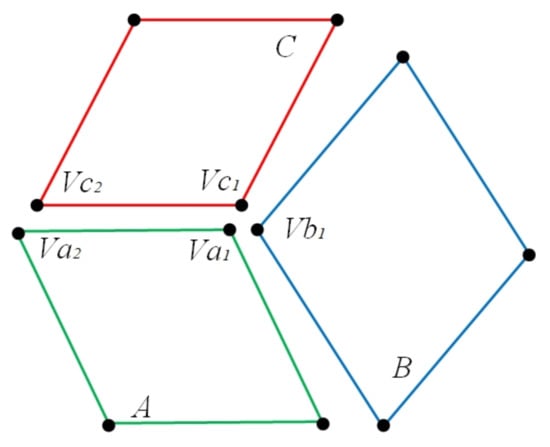
Figure 2.
Graphic illustration of the two types of topological relations. In polygons A, B, and C, if edge (Va1, Va2) matches edge (Vc1, Vc2), then the polygon pair (A, C) is considered to be pairwise adjacent. If vertices Va1, Vb1, and Vc1 are matched with each other, then polygon triplet (A, B, C) is considered to intersect at the common point of the three supporting planes.
Although photogrammetric point clouds can be noisy or partly missing, large planar structures that are well sampled are still reliable for fitting planes and recovering boundaries. Similar to the work by Arikan et al. [53], vertex–vertex matches (VVMs) and vertex–edge matches (VEMs) between two polygons are searched to determine their pairwise adjacency. To obtain robust estimations, the maximal search radius, as described by Arikan et al. [53], should be relatively low (in this paper, it is set to be twice the average point spacing).
Edge–edge matches are derived from VVMs and/or VEMs. In this work, the adjacency between two non-parallel polygons, Polyi and Polyj, is verified by finding at least one pair of edges from the two polygons that satisfy the following criteria:
- (1)
- The two edges are parallel or collinear.
- (2)
- Two VVMs, or one VVM and one VEM, or two VEMs are found for them.
Note that, if more than two edges are found to satisfy the first criteria, all of the possible combination pairs should be tested if they satisfy the second criteria of edge–edge matches. Then, to detect plane triplets of interest, an undirected graph G(V, E), as shown in Figure 3, is generated by setting each polygon as a vertex (the blue dots), with the edge between two vertices indicating matching relationships of the two polygons. As the intersection of three non-parallel polygons can be defined without ambiguity, the shortest closed cycles are searched in the graph G(V, E) [51], and those with the shortest walk of the three indicate an underlying intersection of a triplet of polygons if none are parallel (the red triangles).

Figure 3.
Graphic illustration of polygons and their matching relations. The blue dots represent polygons while the black lines between two dots indicate that they are matched with each other. The red triangles indicate the intersections of three non-parallel polygons.
3.3. Building Model Reconstruction with Initial Topology Constraints
In the previous stage, the adjacency relations between different planar primitives were partially recovered. A set of adjacent planar polygon pairs and a set of intersecting non-parallel polygon triplets are obtained. So, the topology relationship between different planar polygons is divide into two parts: the confident part and the ambiguous part.
In this stage, we incorporate these relations to produce candidate faces and constraints for generating the final building model. Unlike previous work which generates candidate faces by simply intersecting detected planar segments, we embed the recovered topological relations in this process to (1) generate more purposeful candidate faces, and (2) reduce the size of unknown parameters in the energy function. After that, the recovered topology is used to guide the candidate selection process as soft energy functions and hard constraints to obtain better reconstructed models with less artifact and in remarkable running time.
3.3.1. Candidate Deduction with Topological and Spatial Hints
Given a set of boundary polygons with base planes, use of their pairwise intersections is a simple strategy for generating redundant candidate faces. However, the drawback is that the number of candidate faces increases substantially with increases in the initial number of detected polygons. In addition, artifactual faces that are obviously invalid may survive in the reconstructed models. Instead of pairwise intersection of detected planar segments purely, in this paper, we conduct the candidate generation process based on three assumptions:
- (1)
- For adjacent polygon pairs, the candidate faces in each polygon plane might be bounded by their intersecting lines.
- (2)
- For adjacent non-parallel polygon triplets, the candidate faces in each polygon plane might be bounded by the two other intersecting planes.
- (3)
- The potential intersection points of different polygons might not be far away from their boundaries.
The overall workflow of this process is shown in Figure 4. The planar primitives are first pairwise intersected with each other within the scope of the enlarged bounding box to form over-redundant candidate faces. Then, the candidate faces in each plane are processed separately to eliminate part of them according to the detected topological relations in the previous steps and the spatial hints. After that, the union set of invalid candidates are removed. Finally, the remaining candidates in all planes are merged and those that do not satisfy the two-manifold rules are treated as outliers.
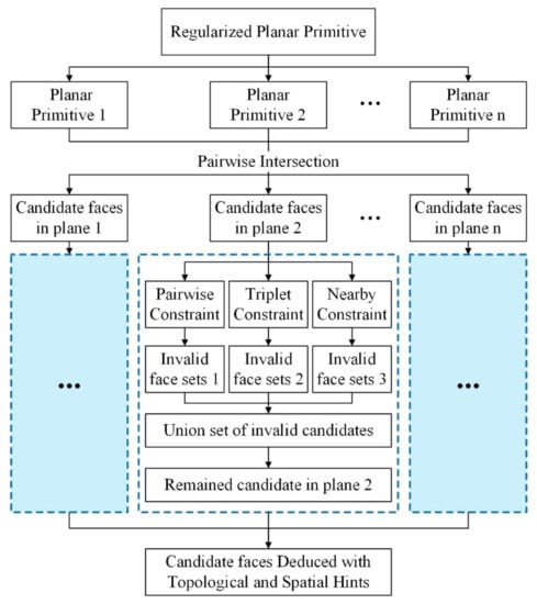
Figure 4.
Overall workflow of the proposed candidate face deduction method.
To swiftly eliminate invalid faces in a plane, π, we divide the candidate faces, FP, in π into three categories, which are marked by green, orange, and gray solid circles in Figure 5. The first category (FPCover) includes faces that share common areas with the detected primitives in the 2D space, these faces are highly confident candidates. The second category (FPNear) includes faces which are not far from the covering area of the detected primitives and are treated as potential candidates. The rest of the faces (FPInvalid) in this plane are labeled as invalid and should be rejected.

Figure 5.
Illustration of the three constraints used to reduce the number of candidate faces. (a): Pairwise Constraint; (b): Triplet Constraint; (c): Nearby Constraint. The red lines depict a simplified boundary polygon A in its supporting plane πA, and the blue lines which separate the plane into several candidate faces are the intersection of other planes in this plane. The green, orange, and gray solid circles indicate the status of the occupied faces as Cover, Near, and Invalid, respectively.
Based on the above assumptions, three types of constraints are used to classify the candidate faces obtained by brutal intersection, namely the pairwise constraint (PC), triplet constraint (TC), and nearby constraint (NC).
Pairwise Constraint: All matched polygon pairs, in which the current one involved should go through this process. As shown in Figure 5a, consider a polygon A with supporting plane πA. If a polygon pair (A, B) is matched in the previous steps, eA is the matched edge in polygon A, and the two supporting planes intersect at line lAB. Theoretically, if the two vertices of eA are both on the convex hull of polygon A, the candidate faces in πA should be bounded by lAB. Then, the candidate faces in πA are labeled as covered (green dot) and invalid (gray dot) respectively, according to their intersection relationship with polygon A. Note that the same process would be done for polygon B in its supporting plane πB. If both polygon A and polygon B are bounded by the intersection line lAB, a sharp edge is implicitly reconstructed in the building model.
Triplet Constraint: All matched polygon triplets, in which the current one involved should go through this process. As shown in Figure 5b, consider a polygon A with supporting planes πA, and a detected polygon triplet (A, B, C), whereby the projections of supporting planes of polygon B and C in πA are two lines, lAB and lAC. Thus, the intersection of lAB and lAC divides πA into four parts. Ideally, if polygon A is located in only one of the four parts, we could bound the candidate faces in πA by the boundaries of the intersecting lines. In practice, due to the presence of noise in point clouds and the errors accumulated in the processing steps, we consider polygon A to be in only one of the four parts when the area percentage of A in this part is larger than a given threshold (e.g., 95%). Then, the candidate faces in πA are restricted to being in this part only. The same verification procedure is also performed for polygons B and C in their supporting planes, respectively. The best situation is that all three polygons are bounded by the two other planes, and a corner point at which all three planes intersect is implicitly reconstructed to bound the building model.
Nearby Constraint: As shown in Figure 5c, for a given polygon A with supporting plane πA, a haphazard pairwise intersection may result in large numbers of invalid candidate faces. Firstly, faces that share common areas with polygon A in the 2D space (πA) are labeled as Covered. Then, the remained faces that share at least one edge with the candidate faces in the first category or at least one vertex that is close to (a distance lower than a given threshold, e.g., 2 m) the vertices of all of the polygons in the first category are labelled as Near. The rest of the faces in this plane are labeled as Invalid.
The union set of invalid candidate faces are rejected from the candidate pool and those that do not satisfy the two-manifold rules are also labeled as Invalid, so the recovered adjacency information in the Section 3.2 is embedded, so that the candidate faces in the confident part are concise and the redundant candidates are mainly in the ambiguous part.
3.3.2. Face Selection with Initial Constraints
In this step, a subset of candidate faces is selected to establish the final building model, which prefers some properties and satisfies certain constraints. To find the optimal configuration of candidate faces, similar to the PolyFit framework [10], we use a binary linear programming approach to quantify the favored properties of the reconstructed model while imposing certain hard constraints. The optimization model contains the binary variables shown in Equation (3) below, which was first developed by Nan and Wonka [10]:
where xf and xe indicate faces in the face pool (F) constructed by all of the candidate faces or an edge in the edge pool (E) that includes all of the associated edges of the faces in the face pool that is selected or not, and xes indicates whether the edge is sharp or not. In this work, four properties are favored:
Property 1: Faces supported by a large number of points are favored.
In Equation (4), p stands for the points in detected primitives, f donates a face of the candidate face pool (F), planef represents the regularized 3D plane that supports face f, projplane-f(p) is the 2D projection of a 3D point p onto the supporting plane of polygon A (πA), dis(p, planef) is the unsigned perpendicular distance from point p to πA, ε is a pre-defined distance tolerance, and num(•) is the size of the set.
Property 2: Faces with a high proportion of their area covered by supporting points are favored.
This property is quantified by the ratio of overlapped area in candidate face with the boundary polygon of the supporting points [10]. In Equation (5), P is a 2D polygon consisting of the boundary of the supporting points for face f and area(•) is the area of the closed polygon. Both of the areas are calculated in 2D space (the supporting plane of face f). Equations (4) and (5) are used to determine the degree to which the data fit the candidate faces, whereby the lower the values, the better the data fit.
Property 3: Intersecting faces in a PC or TC are preferably selected.
In Equation (6), Θ(•) is the confidence coefficient of face f and η is a non-negative constant (set as 1 in all the experiments in this paper) that increases the confidence coefficient values for certain faces.
Property 4: Sharp edges associated with two polygons in a PC or TC are favored.
This property is measured by the overlapped ratio of the sharp edge with the share section of the two matched edges. In Equation (7), e stands for an edge which connects two faces, eP1 and eP2 are the projections of two matched edges (if they matched as PC or TC) on the intersecting line of their corresponding planes, and length(•) represents the unsigned length of the segments. Longer overlapping ratio is preferred. Hence, the following energy function is defined:
The first term in Equation (8) measures the degree to which the properties fit the candidate faces, and the second term measures that for their related edges, ω stands for the corresponding weight. As given in Equation (9), the data fitting degree of a face is composed of two parts, one for point number (Epts), the other one for point coverage (Ecover). Larger number of inlier points and bigger area of face coverage is preferred. The denominator Θ(f) are used to give larger opportunities for faces involved in a PC or TC. In the paper, the weights of the three energy forms, Eedge, Eptd, and Ecovrt, are set as identical.
In addition, three constraints are imposed to strengthen the topologic and geometric features of the building model:
Constraint 1: An edge must be selected when one of its associated faces is selected.
Constraint 2: When an edge is selected, it connects only two candidate faces.
Constraint 3: The edges associated with two polygons in a PC or TC should be sharp.
Properties 1 and 2 and Constraints 1 and 2 are similar to those reported by Nan and Wonka [10] to ensure a watertight polygonal building model, whereas Properties 3 and 4 and Constraint 3 enforce the recovered topology described in Section 3.2 to realize favorable models. The above objectives and constraints are formulated as a binary linear programming problem that can be minimized using existing solvers [54]. Lastly, the selected faces are combined to yield the final building model.
4. Experimental Analysis
4.1. Test Data Description and Experimental Settings
To test the performance of the proposed methods, we made qualitative and quantitative comparisons of the reconstruction quality and computational cost of our method with those of some state-of-the-art (SOTA) methods. The photogrammetric point clouds of the aerial oblique images of typical buildings in Shenzhen, China, were incorporated in the experiments. The original images are captured from five directions (one vertical and four tilt views), so the building façades are (partially) visible. The image overlap is approximately 60% to 80%. Image orientation and dense image matching are accomplished by existing solutions in Context Capture. After that, point clouds of single buildings are manually extracted by drawing 2D bounding boxes. The major components of buildings are visible, and the roof structures are well-sampled. But there are also some missing and imperfect areas due to occlusions and unfavorable lighting conditions in the lower parts of the buildings. The point clouds are shown in Figure 6, while Table 1 lists basic information related to the test data.
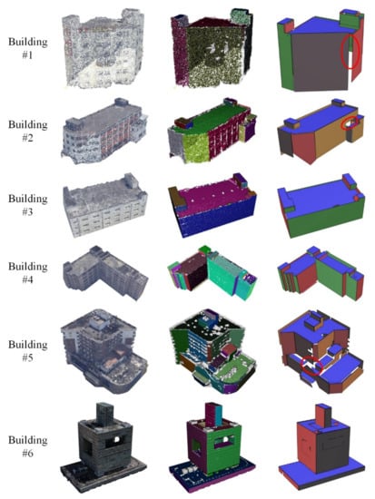
Figure 6.
Photogrammetric point clouds used in the experiments. The row numbers correspond to the building IDs. From left to right, the columns show the original point clouds, the segmented planar primitives, and the extracted outer boundaries of each primitive.

Table 1.
Basic information related to the test data.
Starting with the single point clouds of a building, we used the region-growing method to identify the planar segments. Then, the boundaries of the segments were traced and regularized to concisely abstract the initial building. As plane detection and regularization were beyond the scope of this study, we set the planar segments and their regularized boundaries as inputs in our experiments, which could be generated by an existing method [43]. Figure 6 shows the original point clouds, the detected planes, and the regularized boundaries. As shown in Figure 6, the regularized boundaries of detected planar primitives could preferably represent building outlines at large primitives which are well-sampled. Meanwhile, in areas with data insufficiency (e.g., under sampling or noisy), the recovered boundaries are rather ambiguous, and even some gaps occurred (as pointed out by the circles).
Because PolyFit [10] is the method most closely related to ours, we first qualitatively and quantitatively compared our method with PolyFit with respect to geometric quality and computational efficiency. Since the ground truth 3D models are not available in this area, geometric quality of reconstructed models was determined based on a visual comparison, cloud-to-mesh (C2M) distance statistics, and mesh-to-cloud (M2C) distance statistics. C2M distances are calculated by projecting the original points to their nearest faces in the 3D model, and M2C distances are estimated by first sampling the 3D model and then calculating the cloud-to-cloud distances between the sampled and original point clouds. For C2M distances, a lower value means better data fitting degree, meanwhile, for M2C distances, a lower value means fewer artifacts in the model. For both of the two values, the lower is the better. Besides, computational efficiency is determined by the recorded running time of each step in generating 3D building models. Comparisons with two other SOTA building model reconstruction methods are also presented.
4.2. Comparison with PolyFit
Figure 7, Figure 8, Figure 9, Figure 10, Figure 11 and Figure 12 show the intermediate candidates generated by the proposed and PolyFit methods, as well as the final reconstructed models. Table 2 provides basic information about the candidates and final results, along with the computational costs of the reconstruction process. At first glance, we can observe that the candidate faces generated by the proposed method are more concise than those produced by PolyFit. Some sharp edges and even some building corners were already reconstructed by the proposed adjacency-based topology detection method. As shown in Table 2, the number of candidate faces generated by PolyFit ranged from 1163 to 15,885, whereas those generated by the proposed method ranged between 138 and 2964, which again indicates the efficiency of the process of generating candidate faces by our method. Although the proposed method has to first estimate the adjacency relations before computing the candidate faces, the running time in this step (denoted as ADT in Table 2) is relatively fast compared with the computing times of candidate generation (CGT) and model generation (MGT). The total running times (TT) of PolyFit and our proposed method, as shown in Table 2 for all six tested buildings, reveals that our method is substantially faster. For simple buildings with fewer planar faces (e.g., Buildings #1, 2#, and 3#), although our method used only about 84.2% to 35.6% of the running time that PolyFit did, the computing times are both in the second level. As a building became more complicated, the running time for PolyFit increased dramatically because of the geometric growth in the number of candidate faces. For Building #5, PolyFit used more than 10 min, whereas our method only took 26.428 s, only 4.2% of the total time that PolyFit took. And for Building #6, PolyFit took about 37 min, whereas our method accomplished this task in 37.383 s, nearly 60 times faster than PolyFit.
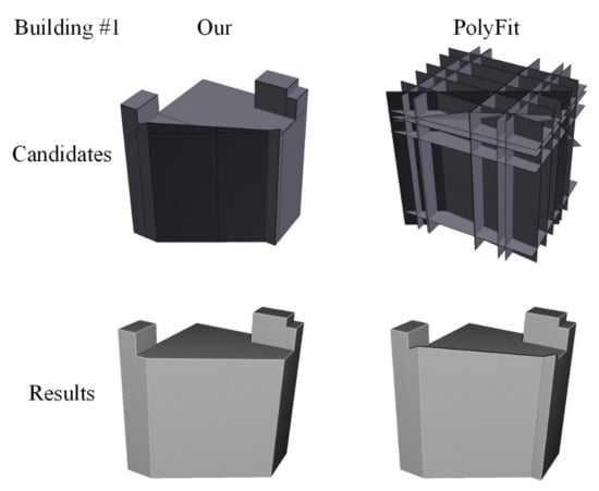
Figure 7.
Comparison of candidate faces and resulting models generated by the proposed method and PolyFit [10] for Building #1.
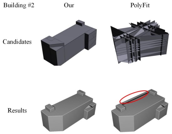
Figure 8.
Comparison of candidate faces and resulting models generated by the proposed method and PolyFit [10] for Building #2.
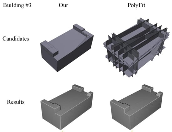
Figure 9.
Comparison of candidate faces and resulting models generated by the proposed method and PolyFit [10] for Building #3.
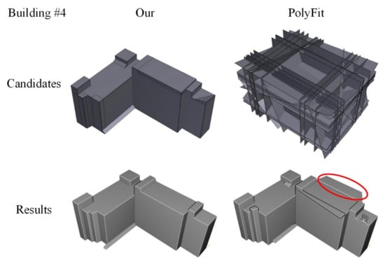
Figure 10.
Comparison of candidate faces and resulting models generated by the proposed method and PolyFit [10] for Building #4.
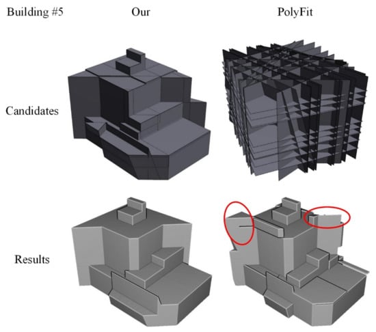
Figure 11.
Comparison of candidate faces and resulting models generated by the proposed method and PolyFit [10] for Building #5.
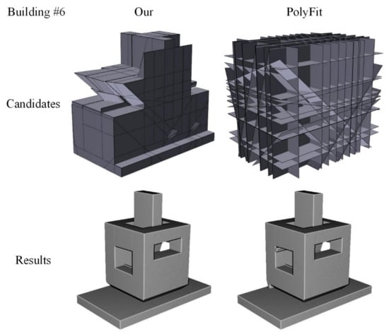
Figure 12.
Comparison of candidate faces and resulting models generated by the proposed method and PolyFit [10] for Building #6.
Table 2.
Quantitative statistics on data and computation cost. BID: Building ID; Can. No.: Number of Candidate faces; Res. No.: Number of resulting faces; ADT: Time for adjacency estimation; CGT: Time for candidate generation; MGT: Time for resulting Model Generation; TT: Total time.
In addition, in Buildings #2, #4, and #5, there are obvious artifacts in the final building models generated by PolyFit as compared with the original point clouds shown in Figure 6. This is a side effect of candidate generation based on the intersections of all potential planar segments. In contrast, by utilizing constraints derived from adjacency information, these artifacts are avoided or alleviated in both candidate generation and candidate selection stages. To verify the objective data fidelity of the reconstructed building models quantitatively, we calculated the mean values of the C2M and M2C distances, as shown in Figure 13. The mean C2M distances for the 3D models generated by PolyFit and the proposed method are all less than 0.30 m, and those for the same buildings are similar. However, for Buildings #2, #4, and #5, the M2C distances generated by PolyFit are significantly greater than those generated by the proposed method. Because greater M2C distances indicates greater data distortion in the final building models, we can infer that the 3D models generated by our method have better geometric accuracy, which also accords with the visual judgments shown in Figure 8, Figure 10 and Figure 11.
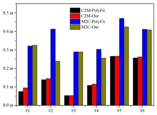
Figure 13.
Mean C2M and M2C distances from Buildings #1 to #6 generated by three-dimensional (3D) models from PolyFit [10] and the proposed method.
4.3. Comparison with Other SOTA Methods
To further evaluate the proposed method, we also conducted an experiment with two SOTA 3D building reconstruction methods, namely the 2.5D dual contouring method (2.5D DC) [55] and the structuring method [56]. As shown in Figure 14, all three methods were able to reconstruct the overall structure of buildings from point clouds. The structuring method also preserved some sharp features, such as the edges and corners of buildings in the models, although some artifactual meshes appeared because of insufficient sampling and data noise. The 2.5D DC method was able to reconstruct building roofs and protect planar structures to a certain degree, but it failed to reconstruct Building #6, which has a typical 3D structure. The mean values of M2C and C2M distances are shown in Figure 15. From Building #1 to Building #4, the C2M distances for all three methods are almost at the same level, ranging from 0.05 to about 0.15 m. Meanwhile, the C2M distance of the proposed method in Building #5 is larger than the two others. The reason is that some small primitives in the original point clouds are not detected and recovered. For Building #6, the C2M value of 2.5D DC is distinctively large since the façades of the building are not well-reconstructed. The mean values of M2C of the three methods are between 0.2 to 0.5 m. Note that, in these three methods, the proposed method is the only one which imposes watertight constraints, so some holes in the point clouds are filled in the output models (e.g., the bottom of the building), which inevitably leads to a higher value of M2C statistics. The situations in Figure 15 reveal that the models recovered by structuring and the proposed method could represent true 3D structures of buildings. Compared with those of the 2.5D DC and structuring methods, the 3D models produced by our proposed method were more concise, with the building surfaces briefly represented by several planar faces. As given in Table 3, the models generated by the proposed method are composed of less faces, over 90% to 99% of faces are reduced when compared with those generated by 2.5D DC and structuring, yielding a concise representation of the building structure which would benefit subsequent applications such as computational simulation in reducing computational costs. Although some small details were smoothed, the models generated by our method have better potential for further interactive editing, if needed, since the main structuring of buildings have been concisely represented without topological conflicts.
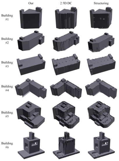
Figure 14.
Comparison of models generated by our proposed method, 2.5D DC method [55], and structuring method [56].

Figure 15.
Mean C2M and M2C distances from Buildings #1 to #6 generated by 3D models from 2.5D DC method [55], structuring method [56], and the proposed method.
Table 3.
Numbers of faces in the reconstructed models by our method, 2.5D DC method [55], and structuring method [56].
5. Discussion
As shown in Figure 7, Figure 8, Figure 9, Figure 10, Figure 11 and Figure 12, the candidates generated by PolyFit are quite superfluous, which makes it hard to recognize the building features (edges, corners) from the candidate faces; meanwhile, the candidates generated by the proposed method have incorporated some recovered topological information, so some of the building features could be visually discovered. Consider the information in Figure 14 and Table 3, one virtue of the proposed method is the concise representation of the original building point clouds with preferred geometry accuracy. In fact, this is also the virtue of PolyFit. Since our method combines the initial recovered topological information, which is obtained by the rule-based method, in the candidate generation and selection process, some unwanted artifacts are alleviated or avoided. The M2C values in Figure 13 also reveal this virtue. Besides, the running time of our method is substantially faster than the traditional hypothesis-based methods, such as PolyFit, especially when the complexity of the building increases. The main difference lies in the MGT process, where a lower ambiguity needs fewer computation times. For a dataset with lower noise and better coverage, it is more likely to extract intact building primitives and to obtain the high-quality regularized boundaries. In these cases, topology relations between primitives are easier to be detected, leading to better initial reconstructions and fewer candidates (see the examples in Figure 7, Figure 8 and Figure 9). Thus, the running times in the candidate selection process are less. In extreme cases with favorable data coverage and sampling density, if all the topological relations of building primitives have been recovered, the candidate faces generated accordingly should equal to the final output model, because there is only one selection combination from which conform all the properties in the energy equations and constraints. Conversely, if the building primitives are not well detected because of data quality (or some other reasons), the adjacency detection process may only work in a small part of areas. Then, the number of generated candidates of our algorithm would increase, leading to longer MGTs and, maybe, some unexpected artifactual structures in the building models. In the most unfortunate cases where no topology has been recovered in the first stage of our algorithm, the proposed method would degenerate to a pure hypothesis-based reconstruction method, similar to PolyFit.
6. Conclusions
In this work, we proposed a novel method for efficient reconstructing building models from photogrammetric point clouds obtained from aerial oblique images in a two-stage topology recovery process which combined the rule-based and the hypothesis-based methods. Given the point clouds of a single building, planar primitives and their corresponding boundaries are extracted and regularized to obtain abstracted building counters. In the first stage, the adjacency relations between different polygons are estimated based on their spatial consistency and mutual regularity to form initial reconstruction. In the second stage, the candidate faces of the building model are generated by the pairwise planar intersections along with three constraints, namely pairwise constraint, triplet constraint, and nearby constraint, derived from the recovered topology. Lastly, the optimal combination of candidate faces is selected by solving a binary linear programming problem that shapes the favored properties under certain constraints. An experimental comparison of our method with three SOTA methods revealed that the proposed method could efficiently reconstruct 3D building models in several seconds and produce concise models with preferred data fidelity and geometric accuracy at the decimeter level. Detailed comparison with PolyFit indicated the high efficiency of the proposed method in reconstructing complex building models and showed promising prospect for this method in 3D city environmental applications. The advantage of the proposed methods is the ability to handle point clouds with various noises in the reconstruction process. However, when the point clouds have large holes or extensively missing areas, the recovered models by our method may degenerate to those constructed by PolyFit, which is a disadvantage. Besides, if the density of the input point clouds is too low, the boundaries extracted from the building primitives may become unstable as well as the initial topology estimation. In future works, methods for incorporating multi-scale primitives and 2D features from oriented images should be developed to handle the situation with low point density and to achieve more detailed reconstruction.
Author Contributions
Conceptualization, L.X. and W.W.; methodology, L.X. and Q.Z.; software, L.X. and H.H.; validation, S.T., Y.L. and Y.Z.; formal analysis, Q.Z. and X.L.; supervision, R.G. All authors wrote the manuscript. All authors have read and agreed to the published version of the manuscript.
Funding
This work was supported by National Key R&D Program of China (2019YFB210310, 2019YFB2103104), the National Natural Science Foundation of China (No.42001407, No.41971341, No. 41971354, 41801392), the Open Fund of Key Laboratory of Urban Land Resources Monitoring and Simulation, MNR (KF-2019-04-042, KF-2019-04-019), the Guangdong Basic and Applied Basic Research Foundation (2019A1515110729, 2019A1515010748, 2019A1515011872), and the Open Research Fund of State Key Laboratory of Information Engineering in Surveying Mapping and Remote Sensing, Wuhan University (No. 20E02).
Acknowledgments
We would like to thank Liangliang Nan, Florent Lafarge and Qianyi Zhou for providing the source codes or executable programs for experimental comparison.
Conflicts of Interest
The authors declare no conflict of interest.
Abbreviations
| LoD | Level of Detail |
| CityGML | City Geography Markup Language |
| LiDAR | Light Detection And Ranging |
| SfM | Structure-from-Motion |
| MVS | Multi-View Stereo |
| RANSAC | RANdom Sample Consensus |
| BSP | Binary Space Partitioning |
| RTG | Roof Topology Graph |
| VVM | Vertex–Vertex Match |
| VEM | Vertex–Edge Match |
| PC | Pairwise Constraint |
| TC | Triplet Constraint |
| NC | Nearby Constraint |
| C2M | Cloud to Mesh |
| M2C | Mesh to Cloud |
References
- Tan, Z.; Lau, K.K.-L.; Ng, E. Planning strategies for roadside tree planting and outdoor comfort enhancement in subtropical high-density urban areas. Build. Environ. 2017, 120, 93–109. [Google Scholar] [CrossRef]
- Wang, S.; Cai, G.; Cheng, M.; Junior, J.M.; Huang, S.; Wang, Z.; Su, S.; Li, J. Robust 3D reconstruction of building surfaces from point clouds based on structural and closed constraints. ISPRS J. Photogramm. Remote Sens. 2020, 170, 29–44. [Google Scholar] [CrossRef]
- Badach, J.; Voordeckers, D.; Nyka, L.; Van Acker, M. A framework for air quality management zones—Useful GIS-based tool for urban planning: Case studies in Antwerp and Gdańsk. Build. Environ. 2020, 174, 106743. [Google Scholar] [CrossRef]
- Biljecki, F.; Stoter, J.; LeDoux, H.; Zlatanova, S.; Çöltekin, A. Applications of 3D city models: State of the art review. ISPRS Int. J. Geo-Inf. 2015, 4, 2842–2889. [Google Scholar] [CrossRef]
- Toschi, I.; Ramos, M.M.; Nocerino, E.; Menna, F.; Remondino, F.; Moe, K.; Poli, D.; Legat, K.; Fassi, F. Oblique photogrammetry supporting 3D urban reconstruction of complex scenarios. ISPRS Arch. 2017, XLII-1/W1, 519–526. [Google Scholar] [CrossRef]
- Yu, D.; Ji, S.; Liu, J.; Wei, S. Automatic 3D building reconstruction from multi-view aerial images with deep learning. ISPRS J. Photogramm. Remote Sens. 2021, 171, 155–170. [Google Scholar] [CrossRef]
- Liu, X.; Zhang, Y.; Ling, X.; Wan, Y.; Liu, L.; Li, Q. TopoLAP: Topology recovery for building reconstruction by deducing the relationships between linear and planar primitives. Remote Sens. 2019, 11, 1372. [Google Scholar] [CrossRef]
- Awrangjeb, M.; Gilani, S.A.N.; Siddiqui, F.U. An effective data-driven method for 3D building roof reconstruction and robust change detection. Remote Sens. 2018, 10, 1512. [Google Scholar] [CrossRef]
- Jarząbek-Rychard, M.; Borkowski, A. 3D building reconstruction from ALS data using unambiguous decomposition into elementary structures. ISPRS J. Photogramm. Remote Sens. 2016, 118, 1–12. [Google Scholar] [CrossRef]
- Nan, L.; Wonka, P. PolyFit: Polygonal Surface Reconstruction from Point Clouds. In Proceedings of the 2017 IEEE International Conference on Computer Vision (ICCV), Venice, Italy, 22–29 October 2017; pp. 2372–2380. [Google Scholar]
- Verdie, Y.; Lafarge, F.; Alliez, P. LOD generation for urban scenes. ACM Trans. Graph. 2015, 34, 1–14. [Google Scholar] [CrossRef]
- Xiong, B.; Elberink, S.O.; Vosselman, G. A graph edit dictionary for correcting errors in roof topology graphs reconstructed from point clouds. ISPRS J. Photogramm. Remote Sens. 2014, 93, 227–242. [Google Scholar] [CrossRef]
- Xu, B.; Jiang, W.; Li, L. HRTT: A hierarchical roof topology structure for robust building roof reconstruction from point clouds. Remote Sens. 2017, 9, 354. [Google Scholar] [CrossRef]
- Ochmann, S.; Vock, R.; Klein, R. Automatic reconstruction of fully volumetric 3D building models from oriented point clouds. ISPRS J. Photogramm. Remote Sens. 2019, 151, 251–262. [Google Scholar] [CrossRef]
- Gruen, A.; Schubiger, S.; Qin, R.; Schrotter, G.; Xiong, B.; Li, J.; Ling, X.; Xiao, C.; Yao, S.; Nuesch, F. Semantically enriched high resolution LoD3 building model generation. ISPRS Int. Arch. Photogramm. Remote Sens. Spat. Inf. Sci. 2019, XLII-4/W15, 11–18. [Google Scholar] [CrossRef]
- Wen, X.; Xie, H.; Liu, H.; Yan, L. Accurate reconstruction of the LoD3 building model by integrating multi-source point clouds and oblique remote sensing imagery. ISPRS Int. J. Geo-Inf. 2019, 8, 135. [Google Scholar] [CrossRef]
- Gröger, G.; Plümer, L. CityGML–Interoperable semantic 3D city models. ISPRS J. Photogramm. 2012, 71, 12–33. [Google Scholar] [CrossRef]
- Zhang, K.; Yan, J.; Chen, S.-C. Automatic construction of building footprints from airborne LiDAR data. IEEE Trans. Geosci. Remote Sens. 2006, 44, 2523–2533. [Google Scholar] [CrossRef]
- Zhao, Z.; Duan, Y.; Zhang, Y.; Cao, R. Extracting buildings from and regularizing boundaries in airborne LiDAR data using connected operators. Int. J. Remote Sens. 2016, 37, 889–912. [Google Scholar] [CrossRef]
- Chen, Q.; Wang, L.; Waslander, S.L.; Liu, X. An end-to-end shape modeling framework for vectorized building outline generation from aerial images. ISPRS J. Photogramm. Remote Sens. 2020, 170, 114–126. [Google Scholar] [CrossRef]
- Widyaningrum, E.; Gorte, B.; Lindenbergh, R. Automatic building outline extraction from ALS point clouds by ordered points aided hough transform. Remote Sens. 2019, 11, 1727. [Google Scholar] [CrossRef]
- Vosselman, G. Building reconstruction using planar faces in very high density height data. ISPRS Arch. 1999, 32, 87–94. [Google Scholar]
- Sohn, G.; Huang, X.; Tao, V. Using a binary space partitioning tree for reconstructing polyhedral building models from airborne LiDAR data. Photogramm. Eng. Remote Sens. 2008, 74, 1425–1438. [Google Scholar] [CrossRef]
- Yang, B.; Huang, R.; Li, J.; Tian, M.; Dai, W.; Zhong, R. Automated reconstruction of building LoDs from airborne LIDAR point clouds using an improved morphological scale space. Remote Sens. 2016, 9, 14. [Google Scholar] [CrossRef]
- Kurdi, F.T.; Awrangjeb, M.; Munir, N. Automatic filtering and 2D modeling of airborne laser scanning building point cloud. Trans. GIS 2021, 25, 164–188. [Google Scholar] [CrossRef]
- Kurdi, F.T.; Awrangjeb, M. Automatic evaluation and improvement of roof segments for modelling missing details using Lidar data. Int. J. Remote Sens. 2020, 41, 4702–4725. [Google Scholar] [CrossRef]
- Song, J.; Xia, S.; Wang, J.; Chen, D. Curved buildings reconstruction from airborne LiDAR data by matching and deforming geometric primitives. IEEE Trans. Geosci. Remote Sens. 2021, 59, 1660–1674. [Google Scholar] [CrossRef]
- Kulawiak, M.; Lubniewski, Z. Improving the accuracy of automatic reconstruction of 3D complex buildings models from airborne LiDAR point clouds. Remote Sens. 2020, 12, 1643. [Google Scholar] [CrossRef]
- Kim, K.; Shan, J. Building roof modeling from airborne laser scanning data based on level set approach. ISPRS J. Photogramm. Remote Sens. 2011, 66, 484–497. [Google Scholar] [CrossRef]
- Poullis, C.; You, S. Photorealistic large-scale urban city model reconstruction. IEEE Trans. Vis. Comput. Graph. 2008, 15, 654–669. [Google Scholar] [CrossRef]
- Henn, A.; Gröger, G.; Stroh, V.; Plümer, L. Model driven reconstruction of roofs from sparse LiDAR point clouds. ISPRS J. Photogramm. Remote Sens. 2013, 76, 17–29. [Google Scholar] [CrossRef]
- Lafarge, F.; Descombes, X.; Zerubia, J.; Pierrot-Deseilligny, M. Automatic building extraction from DEMs using an object approach and application to the 3D city modeling. ISPRS J. Photogramm. Remote Sens. 2008, 63, 365–381. [Google Scholar] [CrossRef]
- Cao, R.; Zhang, Y.; Liu, X.; Zhao, Z. 3D building roof reconstruction from airborne LiDAR point clouds: A framework based on a spatial database. Int. J. Geogr. Inf. Sci. 2017, 31, 1359–1380. [Google Scholar] [CrossRef]
- Tarsha Kurdi, F.; Landes, T.; Grussenmeyer, P.; Koehl, M. Model-driven and data-driven approaches using Lidar data: Analysis and comparison. ISPRS Arch. 2007, XXXVI W49A, 1682–1687. [Google Scholar]
- Wang, R.; Peethambaran, J.; Chen, D. LiDAR point clouds to 3D urban models: A review. IEEE J. Sel. Top. Appl. Earth Obs. Remote Sens. 2018, 11, 606–627. [Google Scholar] [CrossRef]
- Lin, Y.; Wang, C.; Cheng, J.; Chen, B.; Jia, F.; Chen, Z.; Li, J. Line segment extraction for large scale unorganized point clouds. ISPRS J. Photogramm. Remote Sens. 2015, 102, 172–183. [Google Scholar] [CrossRef]
- Schnabel, R.; Wahl, R.; Klein, R. Efficient RANSAC for point-cloud shape detection. Comput. Graph. Forum 2007, 26, 214–226. [Google Scholar] [CrossRef]
- Tarsha Kurdi, F.; Landes, T.; Grussenmeyer, P. Hough-transform and extended RANSAC algorithms for automatic detection of 3D building roof planes from LiDAR data. In Proceedings of the ISPRS Workshop on Laser Scanning 2007 and SilviLaser 2007, Espoo, Finland, 12–14 September 2007; Volume 36, pp. 407–412. [Google Scholar]
- Lari, Z.; Habib, A. An adaptive approach for the segmentation and extraction of planar and linear/cylindrical features from laser scanning data. ISPRS J. Photogramm. Remote Sens. 2014, 93, 192–212. [Google Scholar] [CrossRef]
- Lu, X.; Yao, J.; Tu, J.; Li, K.; Li, L.; Liu, Y. Pairwise linkage for point cloud segmentation. ISPRS Ann. 2016, III-3, 201–208. [Google Scholar]
- Sampath, A.; Shan, J. Building boundary tracing and regularization from airborne LiDAR point clouds. Photogramm. Eng. Remote Sens. 2007, 73, 805–812. [Google Scholar] [CrossRef]
- Li, M.; Nan, L.; Smith, N.; Wonka, P. Reconstructing building mass models from UAV images. Comput. Graph. 2016, 54, 84–93. [Google Scholar] [CrossRef]
- Xie, L.; Zhu, Q.; Hu, H.; Wu, B.; Li, Y.; Zhang, Y.; Zhong, R. Hierarchical regularization of building boundaries in noisy aerial laser scanning and photogrammetric point clouds. Remote Sens. 2018, 10, 1996. [Google Scholar] [CrossRef]
- Chen, D.; Wang, R.; Peethambaran, J. Topologically aware building rooftop reconstruction from airborne laser scanning point clouds. IEEE Trans. Geosci. Remote Sens. 2017, 55, 7032–7052. [Google Scholar] [CrossRef]
- Chen, D.; Zhang, L.; Mathiopoulos, P.T.; Huang, X. A Methodology for automated segmentation and reconstruction of urban 3D buildings from ALS point clouds. IEEE J. Sel. Top. Appl. Earth Obs. Remote Sens. 2014, 7, 4199–4217. [Google Scholar] [CrossRef]
- Benciolini, B.; Ruggiero, V.; Vitti, A.; Zanetti, M. Roof planes detection via a second-order variational model. ISPRS J. Photogramm. Remote Sens. 2018, 138, 101–120. [Google Scholar] [CrossRef]
- Sampath, A.; Shan, J. Segmentation and reconstruction of polyhedral building roofs from aerial lidar point clouds. IEEE Trans. Geosci. Remote Sens. 2010, 48, 1554–1567. [Google Scholar] [CrossRef]
- Elberink, S.O.; Vosselman, G. Building reconstruction by target based graph matching on incomplete laser data: Analysis and limitations. Sensors 2009, 9, 6101–6118. [Google Scholar] [CrossRef]
- Hu, H.; Chen, C.; Wu, B.; Yang, X.; Zhu, Q.; Ding, Y. Texture-aware dense image matching using ternary census transform. ISPRS Ann. 2016, III-3, 59–66. [Google Scholar]
- Wu, B.; Xie, L.; Hu, H.; Zhu, Q.; Yau, E. Integration of aerial oblique imagery and terrestrial imagery for optimized 3D modeling in urban areas. ISPRS J. Photogramm. Remote Sens. 2018, 139, 119–132. [Google Scholar] [CrossRef]
- Perera, G.S.N.; Maas, H.-G. Cycle graph analysis for 3D roof structure modelling: Concepts and performance. ISPRS J. Photogramm. Remote Sens. 2014, 93, 213–226. [Google Scholar] [CrossRef]
- Bauchet, J.-P.; Lafarge, F. Kinetic shape reconstruction. ACM Trans. Graph. 2020, 39, 1–14. [Google Scholar] [CrossRef]
- Arikan, M.; Schwärzler, M.; Flöry, S.; Wimmer, M.; Maierhofer, S. O-snap: Optimization-based snapping for modeling architecture. ACM Trans. Graph. 2013, 32, 6. [Google Scholar] [CrossRef]
- Gamrath, G.; Anderson, D.; Bestuzheva, K.; Chen, W.; Eifler, L.; Gasse, M.; Gemander, P.; Gleixner, A.; Gottwald, L.; Halbig, K.; et al. The SCIP Optimization Suite 7.0; Optimization Online; Zuse Institut: Berlin, Germany, 2020. [Google Scholar]
- Zhou, Q.-Y.; Neumann, U. 2.5D Dual Contouring: A robust approach to creating building models from aerial LiDAR point clouds. In Constructive Side-Channel Analysis and Secure Design, Proceedings of the 3rd International Workshop, COSADE, Darmstadt, Germany, 3–4 May 2012; Springer: Berlin, Germany, 2012. [Google Scholar]
- Lafarge, F.; Alliez, P. Surface reconstruction through point set structuring. Comput. Graph. Forum 2013, 32, 225–234. [Google Scholar] [CrossRef]


Publisher’s Note: MDPI stays neutral with regard to jurisdictional claims in published maps and institutional affiliations. |
© 2021 by the authors. Licensee MDPI, Basel, Switzerland. This article is an open access article distributed under the terms and conditions of the Creative Commons Attribution (CC BY) license (http://creativecommons.org/licenses/by/4.0/).