Article

Deep-Learning-Based Classification of Point Clouds for Bridge Inspection

Department of Architectural Engineering, Chung-Ang University, Seoul 06974, Korea
*
Author to whom correspondence should be addressed.
Remote Sens. 2020, 12(22), 3757; https://doi.org/10.3390/rs12223757
Submission received: 17 October 2020 / Revised: 11 November 2020 / Accepted: 13 November 2020 / Published: 16 November 2020
(This article belongs to the Special Issue 3D City Modelling and Change Detection Using Remote Sensing Data)

Abstract

:
Conventional bridge maintenance requires significant time and effort because it involves manual inspection and two-dimensional drawings are used to record any damage. For this reason, a process that identifies the location of the damage in three-dimensional space and classifies the bridge components involved is required. In this study, three deep-learning models—PointNet, PointCNN, and Dynamic Graph Convolutional Neural Network (DGCNN)—were compared to classify the components of bridges. Point cloud data were acquired from three types of bridge (Rahmen, girder, and gravity bridges) to determine the optimal model for use across all three types. Three-fold cross-validation was employed, with overall accuracy and intersection over unions used as the performance measures. The mean interval over unit value of DGCNN is 86.85%, which is higher than 84.29% of Pointnet, 74.68% of PointCNN. The accurate classification of a bridge component based on its relationship with the surrounding components may assist in identifying whether the damage to a bridge affects a structurally important main component.

Graphical Abstract

1. Introduction

Organization for Economic Cooperation and Development (OECD) countries spend a significant amount of money on infrastructure maintenance to prevent damage and resulting accidents [1]. For example, in 2014, the United States spent 235 million dollars, representing 57% of its infrastructure budget, on maintenance [2] while Japan spent a total of 1.99 billion yen (18.79 billion US dollars) on maintenance in 2017, which was 33% of its public works budget [3]. In South Korea, the deterioration of national infrastructure, much of which was constructed in the 1960s and 1970s, and the subsequent need to repair it is expected to increase [4]. Of the 28,945 infrastructure facilities in Korea, 10,070 are bridges, and 31% of all road bridges were more than 20 years old as of February 2020. Because the proportion of bridges 20 years old or higher will rapidly increase to 70% over the next decade, the number of bridges that require immediate repair due to damage to their main components (i.e., safety class C or lower) is expected to rise [5]. Accordingly, the Korea Ministry of Land, Infrastructure, and Transport is taking proactive measures by carrying out maintenance when damage is in its early stages rather than pursuing conventional reactive maintenance in which damage such as steel corrosion or cracks is repaired after deterioration [6]. Proactive maintenance is estimated to save 828.7 billion won in maintenance costs by 2030 [4]. Because more frequent inspections are required in order to repair early-stage damage, an automated detection method that does not require significant time or effort is required.
Conventional manual maintenance of bridges usually involves four stages. First, skilled workers detect cracks, steel corrosion, and other forms of damage using visual inspection, and the damage is inspected using simple tools such as a crack ruler. Second, the severity and location of the damage are directly recorded using two-dimensional (2D) inspection drawings. Third, the safety class of the damage is evaluated depending both on its severity and on which of the main and/or auxiliary components are damaged. Finally, repairs are carried out to prevent the loss of functionality and durability when the main components are damaged or when there is wide-ranging damage to the auxiliary components. This process, however, requires considerable time and effort because it involves manual inspection, while the damage is recorded in 2D drawings [7]. To overcome this problem, South Korea has established its first basic plan for infrastructure management and aims to introduce a smart maintenance system using unmanned aerial vehicles (UAVs) that acquire images of infrastructure facilities. It also plans to implement a process for recording and storing three-dimensional (3D) information from these facilities within the next five years [6]. Despite the benefits of automation, inspecting damage using images acquired by UAVs, recording the location and severity of the damage as 3D information, and subsequently evaluating the safety classes must still be conducted manually.
Several studies using computer vision to automate procedures currently performed manually have been conducted recently (e.g., [8,9,10,11,12,13,14,15,16,17,18,19,20,21,22]), including those that utilize 3D point cloud data and 2D image information to inspect damage to bridges. Studies utilizing 2D image information include those investigating bridge load estimation [8,9], strain measurement [10,11], displacement measurement [12,13,14], and concrete crack detection [7,15], while 3D point cloud data research has included bridge displacement measurement [16,17], deformation monitoring [18,19], and damage detection [20,21,22]. These studies have successfully identified and inspected damage to local areas but generally fail to identify whether this damage affects the main components, which can reduce the overall durability and functionality of the bridge. Therefore, an approach that can identify the location of damage in 3D space and classify the components involved is required. Some researchers (e.g., [23,24,25]) have attempted to classify 3D point cloud data into their respective components, but their results can only be applied to specific, simple bridge types (e.g., girder bridges with only horizontal and vertical components).
In the present study, we compare models that are capable of classifying components (e.g., abutments, piers, and girders) using point cloud data from various bridge types to allow automated maintenance that is not limited to specific types of bridge. This is achieved by segmenting the point cloud data for each classified bridge component using an optimal algorithm. The structure of the remainder of the paper is as follows. Section 2 presents a review of the research that has classified bridge components within the construction industry, while Section 3 describes the deep-learning models that are compared in this study. Section 4 presents the process used to compare the models, while Section 5 analyzes the comparison results and presents a summary, the limitations, and future research.

2. Related Work

Various studies have proposed methods for automatically inspecting damage in bridge maintenance procedures using 2D image information (e.g., [8,9,10,11,12,13,14,15]) or 3D point cloud data (e.g., [16,17,18,19,20,21,22]). However, identifying whether damage needs to be repaired using automatic inspection has not yet been possible, and the damaged area must be identified in 3D space to determine whether a main component is involved. The use of hard coding for bridge component classification has been suggested [23,24,26], but the segmentation of point cloud data has not been automated in these approaches, and they could only be applied to simple bridge types with perpendicular vertical and horizontal components and no complex shapes.
Segmenting components to automatically classify point cloud data from bridges using the region growing method [27,28] has been proposed. This approach extracts a curved surface and plane by extending seed points into a region until an edge is reached where the change in the vector reaches a certain threshold in the point cloud data, where the seeds are manually or automatically input. A region growing method [29] that transforms the point cloud data into an octree to increase the processing speed has also been proposed. However, when using this method, an object can be over-segmented into multiple regions instead of one due to occlusion.
Some studies have proposed model-based segmentation methods that prevent over-segmentation due to occlusion. Schnabel, et al. [30] proposed a random sample consensus (RANSAC)-based method that compares samples randomly extracted from the point cloud data with a 3D geometry model (e.g., a sphere or cylinder) to form a model at the position where the sum of the distance is minimized. Xu, et al. [31] modified this method into an octree with high processing speed for point cloud data acquired from a construction site. Laefer and Truong-Hong [32] proposed a method for filling occluded regions using a repeated pattern for a grid-like steel structure. However, these model-based methods cannot be applied to bridges that do not have a grid-like structure or a simple geometry (e.g., spherical or cylindrical).
Previous studies on automatically classifying bridge components have not been able to automatically process the segmentation of input data. They can process specific shapes but cannot segment component units or classify component types, thus they cannot be used for the purpose of automating maintenance because the component class that a segmented object belongs to cannot be identified. Kim, Yoon and Sim [25] proposed a framework for segmenting and classifying bridge components by applying the semantic segmentation of point cloud data using PointNet [33], a deep-learning-based algorithm in which data segmentation and classification are carried out simultaneously. PointNet can learn unstructured cloud data, but information on the local relationship between points is not learned and the data are independently learned [34]. The component types in a bridge can vary according to their relationship with surrounding components and the shape information of each component. Therefore, an algorithm capable of accurately classifying and segmenting each component and separating main from auxiliary components is needed to evaluate the safety class of a bridge.

3. Deep-Learning Algorithms

In this study, three deep-learning algorithms were selected to classify the components of bridges. The selection of the three deep-learning algorithms—PointNet, Point Convolutional Neural Network (PointCNN), and Dynamic Graph Convolutional Neural Network (DGCNN)—is based on the following common features:
-
They can handle semantic segmentation problems for point cloud data.
-
They can use irregular point cloud data without converting it into a regular format.
-
They use the same block sampling method introduced by Qi, Su, Mo and Guibas [33].
A brief introduction to each algorithm is given here, while a more detailed explanation can be found in the references [33,35,36,37].

3.1. PointNet

PointNet [33] was the first neural network architecture to directly receive point cloud data as input for learning. It directly uses point cloud data without converting the data into 3D voxels or 2D images at a specific time; this prevents the loss of original information and reduces unnecessary processing time. PointNet uses symmetric functions that output the same results regardless of the input order (i.e., addition and multiplication). As shown in Figure 1, the information for each point is output independently as the values of multiple channels using a multilayer perceptron (MLP), while the max-pooling layer, which is a symmetric function, extracts the largest value for each channel of all output point features independent of the order of the points to accumulate the global features from all input points. Therefore, PointNet can directly label input points by taking into consideration the features of each point and the features of the global shape of the input points.

3.2. PointCNN

PointCNN [35] is designed to learn the local correlation between points in space by generalizing the structure of a convolution neural network (CNN). PointCNN uses untransformed point cloud data in the same way that PointNet does, and it can learn regardless of the input order by generalizing the principle of grid CNNs applied to images and learn the correlation between adjacent points in space. For an image, a CNN generally reduces the input range for each convolution (conv) layer and increases the channels to recursively learn the correlation between evenly arranged data points and their surroundings (Figure 2a). PointCNN also reduces the number of input neighboring points for each layer and increases the channels to recursively learn the correlation with the surrounding points (Figure 2b) but instead uses x-conv, which inputs neighboring points using K-nearest neighbor (KNN), rather than general conv layers to input point cloud data with an irregular format.

3.3. DGCNN

DGCNN [36] is an architecture that can learn local correlations in the same way as a CNN. It also learns the correlations with adjacent points or points with similar features using a dynamic graph for each layer of the network. DGCNN also receives untransformed point cloud data as input similar to PointNet but replaces the MLP with a structure that learns information from adjacent points (Figure 3c). Unlike general CNN architecture, the architecture of DGCNN updates the graph to obtain adjacent points in feature-based Euclidean space for each layer (Figure 3a) and can thus learn edge vectors from different points. Unlike the case where general convolution layers learn the information for the surrounding points along with the center point, edge convolution learns the information for edge vectors directed from the features of the center point toward the features of the surrounding points (Figure 3b). Therefore, DGCNN can learn the features of a greater variety of data than other forms of conventional architecture designed for point clouds.

4. Methodology

4.1. Block Partitioning for Model Input

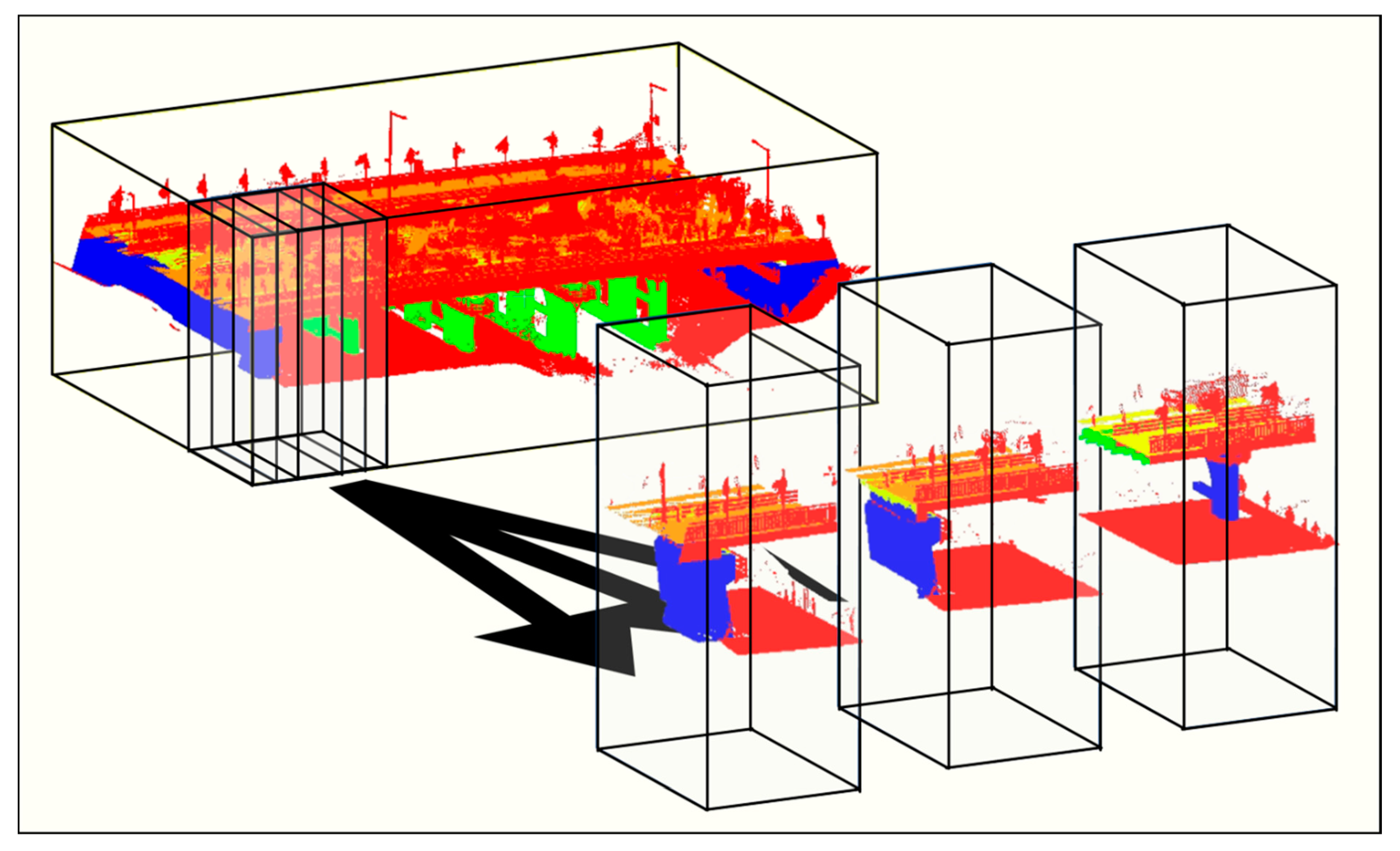
Unlike general 2D image data, point cloud data have an irregular arrangement in 3D space. Therefore, these data are generally converted into regular arrangements, such as 3D voxels or 2D images. Deep-learning algorithms such as PointNet, PointCNN, and DGCNN do not convert the data into regular arrangements, but perform the same process of partitioning the data into blocks of specific sizes. The point cloud data held in each block are free from data loss, and overlapping sections are present between the blocks. Therefore, the classification accuracy of the model can be improved via extensive learning. Point cloud data partitioned in block units retain their irregular arrangement for some sections of a bridge (Figure 4). The size and overlap of the blocks used in partitioning the point cloud data directly affect the number and density of the point cloud data input into the model; this is discussed in the experiments and results in Section 5.

4.2. Performance Measures

In this study, the performance of the semantic segmentation models was evaluated using overall accuracy (OA) and intersection over union (IoU). OA represents the labeling accuracy for all points, while IoU is obtained by measuring the ratio of the intersection and union between real labels and model labels. The two performance measures are calculated as follows:
OA = i = 1 N ( T P i / ( T P i + F N i ) ) / N
IoU = i = 1 N ( T P i / ( T P i + F P i + F N i ) )
where N indicates the number of component classes, and TP represents the number of points for which the real and labeled classification of a component are the same (i.e., true positives). FP represents the number of falsely labeled points that do not belong to a specific component (i.e., false positives), and FN represents the number of points that belong to a specific component but are not labeled as such (i.e., false negatives).

4.3. Cross-Validation

Simple substitution [38], holdout [39], bootstrap [40], and bolstered methods [41] can be used to validate classification models. Of these methods, k-fold cross-validation [42] is the most widely used. K-fold cross-validation uses k − 1 folds for learning and the remaining fold for validation. The average of the results obtained from repeating the aforementioned task k times with different folds each time was used to assess model performance.
In this study, three-fold cross-validation was employed with point cloud datasets of similar sizes. Because point cloud data have unique features and sizes, folds with similar sizes are required. An explanation of the data making up each fold is presented in Section 5.

4.4. Hyperparameter Tuning

The block size and overlap were obtained using three-fold cross-validation and a grid search. The evaluation criterion for the grid search was OA, which indicates the ratio of properly labeled data to total data. The range of the block sizes included multiples of 3 m (3 m, 6 m, 9 m, 12 m, and 15 m) so that the thickest pier (2.5 m) of the bridges from which the data were obtained was included within one block. The overlap ratio is based on the number of times the same point cloud is included in different blocks. For example, the same point cloud can be included in a different block four times (2 × 2) when the overlap ratio is 50%, and 25 times (5 × 5) when it is 80%, which can be entered as learning data in the deep learning model.

5. Experiment and Results

We used a Trimble TX8 laser scanner to acquire data from 27 scans on the average of the three bridges (Figure 5) to compare the performance of the models in classifying the components of the bridges. The errors in the point cloud data acquired at the level 1 stage of the Trimble TX8 equipment were within 2 mm [43]. The automatic plane-based registration method was used for the registration method, using Realworks of Trimble™ [44]. The three bridges from which the scan data were acquired were of different types: a Rahmen, girder, and gravity bridge (Figure 5). The dimension information of the bridges is given in Table 1. Because the bridges have different substructures, the component types making up the bridges are different; therefore, data similar to validation data must be included in the training data. The data from the three bridges were divided into six regions (Table 2), and three-fold cross-validation was employed.
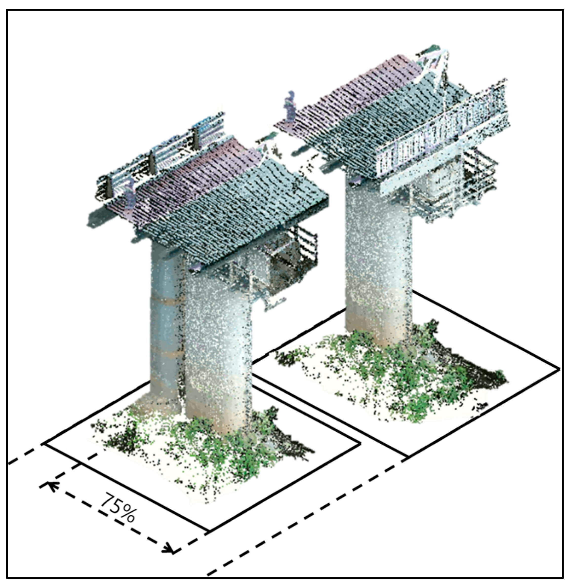
As mentioned in Section 4.1, a grid search and three-fold cross-validation were used to optimize the size and overlap ratio of the blocks input into the three classification models. Optimal values were selected using the grid search of two block-related hyperparameters from among the various parameters used in each model. The range of the block size included multiples of 3 m and the range of overlap ratio included were from 50% (2 × 2 times) to 80% (5 × 5 times). The overlap ratio indicates the extent to which one block and its adjacent blocks overlap (Figure 6), and sufficient training data for the models can be obtained when the overlap ratio increases. The values of hyperparameters not related to blocks are listed in Table 3. Table 4 shows the OA values according to the hyperparameters for each model. DGCNN had the highest OA (94.49%), while PointNet and PointCNN were less accurate at 93.83% and 92.55%, respectively.
As mentioned earlier, three optimized deep-learning models were used to classify the point cloud data of three bridges. Table 5 shows the prediction performance of each model for the validation set based on the IoU for the point cloud data belonging to their respective components. The mean IoU represents the mean of the IoU for all components; DGCNN had the highest mean IoU with 94.49%. The IoU for the abutments (i.e., the vertical components) of DGCNN was higher than that of PointNet by 18.81%. The IoU for the piers of PointNet was relatively high, but this is not because of their excellent classification performance, but because PointNet classified most vertical members as piers. The bridge component classification accuracy of DGCNN, which learns the relationship with the surrounding points along with the position and color information of each point, was higher than PointNet, which learns only the position and color information.
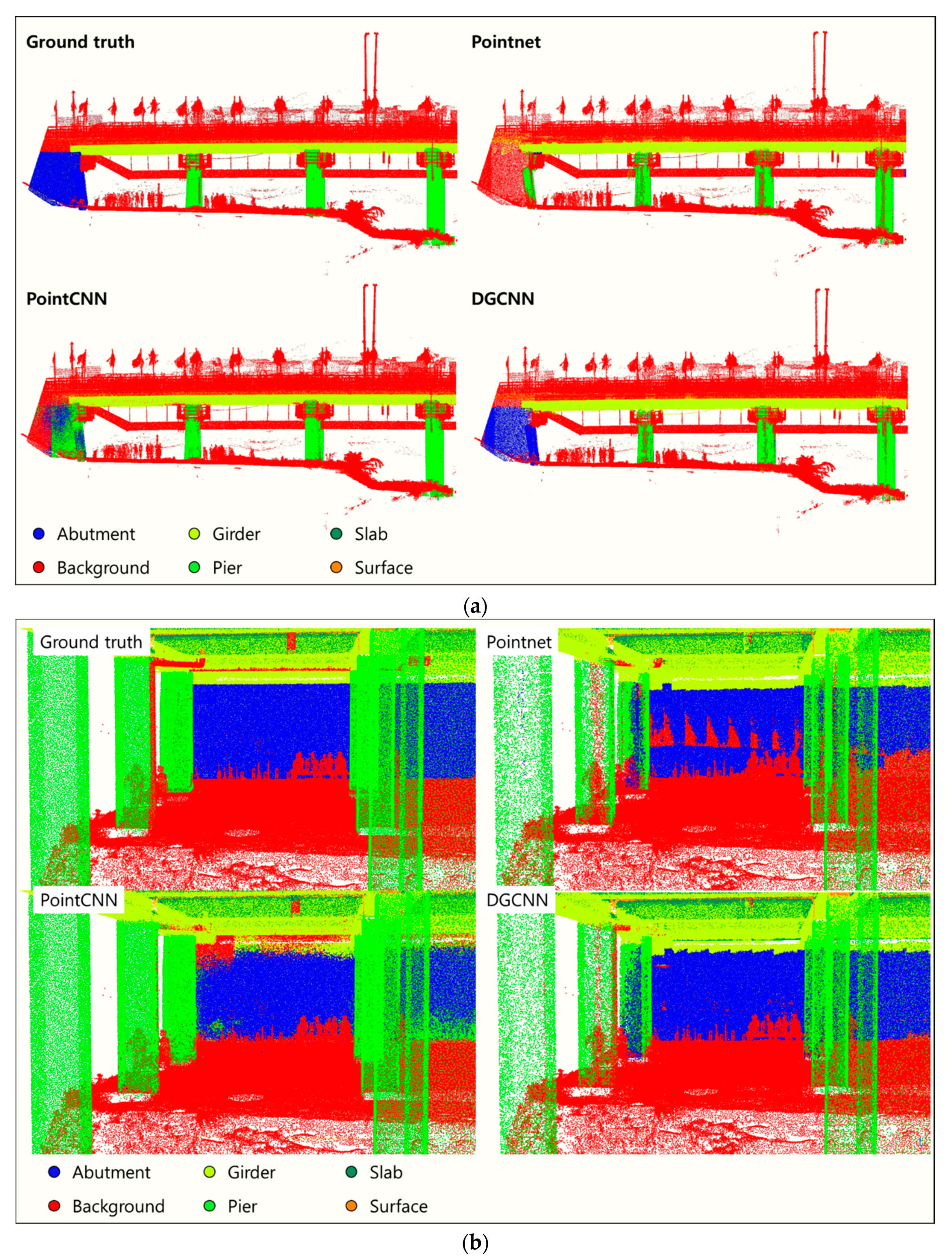
The qualitative results of the three classification models are presented in Figure 7. The color of each point represents the classified component (abutment, background, deck, girder, pier, slab, and surface). PointNet did not accurately classify the piers, abutments, and background located on the same z-axis, whereas the girders were distinguished based on specific z values. PointNet also could not classify the abutments and the columns (Figure 7a). The PointNet network, which learns only the independent features for each point and the global features using symmetric functions on the input points, did not learn the relationship with the surrounding points. In contrast, PointCNN learns the relationship with the adjacent points in the xyz coordinate system and thus accurately classified the background and the girders (i.e., the horizontal components) as well as the piers and abutments (i.e., the vertical components). However, it did not accurately classify the piers and abutments that did not have large differences in the local features (Figure 7a). DGCNN accurately classified the components that were separated from each other such as the piers and abutments because it learned the relationships with points adjacent to each other in xyz space and that were similar based on its self-updated features. However, as shown in Figure 7b, because various self-updated features were used, the edges between the piers and the background were relatively less accurate than with PointCNN.

6. Conclusions

In this study, three deep learning models—PointNet, PointCNN, and DGCNN—were compared to classify the components of bridges. Point cloud data were acquired from a Rahmen bridge, a girder bridge, and a gravity bridge to determine the best performing model for use with various bridge types. Three-fold cross-validation was employed, and OA and IoU were used as performance measures.
DGCNN exhibited higher accuracy (OA: 94.49%; mIoU: 86.85%) than PointNet (OA: 93.83%; mIoU: 84.29%) and PointCNN (OA: 92.55%, mIoU: 76.78%), which has been used in the construction industry. Unlike PointNet, which only learns the global features of the input points and the information of each point, DGCNN, which also learns the information for neighboring points, produced features suitable for the classification of various bridge components as defined by the relationship with the surrounding components.
Accurately classifying bridge components based on their relationship with the surrounding components can assist in identifying whether a structurally important main component is damaged. Thus, the proposed method has the potential for use in automating the storage of information in 3D space that was originally recorded in 2D drawings and in evaluating the safety class of a bridge based on damage information for its main components. However, because the same bridges were used in the learning and validation datasets due to the small number of bridges tested, sufficient data for bridges of the same form need to be procured to establish separate training and validation datasets in future research. In addition, the main regions of each bridge need to be identified for automated bridge safety inspection.

Author Contributions

Conceptualization, H.K. and C.K.; Data curation, H.K. and C.K.; Formal analysis, H.K.; Funding acquisition, C.K; Investigation, H.K. and C.K.; Methodology, H.K. and C.K.; Project administration, C.K.; Resources, H.K. and C.K.; Software, H.K.; Supervision, C.K; Validation, H.K. and C.K.; Visualization, H.K.; Writing—original draft, H.K. and C.K.; Writing—review & editing, C.K. All authors have read and agreed to the published version of the manuscript.

Funding

This study was supported by the Basic Science Research Program through the National Research Foundation of Korea funded by the Ministry of Education (NRF-2018R1D1A1B07049846) and the Chung-Ang University GRS (graduate research scholarship) in 2020.

Conflicts of Interest

The authors declare no conflict of interest.

References

  1. Rothballer, C.; Lam-Frendo, M.; Kim, H. Strategic Infrastructure Steps to Operate and Maintain Infrastructure Efficiently and Effectively; Forum, I.W.E., Ed.; World Economic Forum: Geneva Canton, Switzerland, 2014. [Google Scholar]
  2. Musick, N.; Petz, A. Public Spending on Transportation and Water Infrastructure, 1956 to 2014; Congressional Budget Office, Ed.; US Congressional Budget Office: Washington, DC, USA, 2015. [Google Scholar]
  3. Japanese Public Finance Fact Sheet; Japanese Ministry of Finance (Ed.) Japanese Ministry of Finance: Tokyo, Japan, 2017.
  4. Strategies for National Infrastructure Intelligence for Innovative Growth. (Smart SOC); Korea National Information Society Agency (Ed.) Korea National Information Society Agency: Seoul, Korea, 2017. [Google Scholar]
  5. Korea Infrastructure Safety Corporation Status of Public Facility Safety Management; Korea Infrastructure Safety Corporation: Seoul, Korea, 2020.
  6. The First Basic Plan for Infrastructure Management; Korea Ministry of Land, Infrastructure and Transport (Ed.) Construction Policy Institute of Korea: Seoul, Korea, 2019.
  7. Yang, Y.-S.; Wu, C.-l.; Hsu, T.T.; Yang, H.-C.; Lu, H.-J.; Chang, C.-C. Image analysis method for crack distribution and width estimation for reinforced concrete structures. Automat. Constr. 2018, 91, 120–132. [Google Scholar] [CrossRef]
  8. Chen, Z.; Li, H.; Bao, Y.; Li, N.; Jin, Y. Identification of spatio-temporal distribution of vehicle loads on long-span bridges using computer vision technology. Struct. Control Health Monit. 2016, 23, 517–534. [Google Scholar] [CrossRef]
  9. Pan, Y.; Wang, D.; Shen, X.; Xu, Y.; Pan, Z. A novel computer vision-based monitoring methodology for vehicle-induced aerodynamic load on noise barrier. Struct. Control Health Monit. 2018, 25, e2271. [Google Scholar] [CrossRef]
  10. Dutton, M.; Take, W.A.; Hoult, N.A. Curvature monitoring of beams using digital image correlation. J. Bridge Eng. 2014, 19, 05013001. [Google Scholar] [CrossRef] [Green Version]
  11. Hoult, N.A.; Take, W.A.; Lee, C.; Dutton, M. Experimental accuracy of two dimensional strain measurements using digital image correlation. Eng. Struct. 2013, 46, 718–726. [Google Scholar] [CrossRef]
  12. Lydon, D.; Lydon, M.; Taylor, S.; Del Rincon, J.M.; Hester, D.; Brownjohn, J. Development and field testing of a vision-based displacement system using a low cost wireless action camera. Mech. Syst. Signal Process. 2019, 121, 343–358. [Google Scholar] [CrossRef] [Green Version]
  13. Lee, J.; Lee, K.-C.; Jeong, S.; Lee, Y.-J.; Sim, S.-H. Long-term displacement measurement of full-scale bridges using camera ego-motion compensation. Mech. Syst. Signal Process. 2020, 140, 106651. [Google Scholar] [CrossRef]
  14. Yoon, H.; Shin, J.; Spencer, B.F., Jr. Structural displacement measurement using an unmanned aerial system. Comput.-Aided Civil Infrastruct. Eng. 2018, 33, 183–192. [Google Scholar] [CrossRef]
  15. Kim, H.; Ahn, E.; Cho, S.; Shin, M.; Sim, S.-H. Comparative analysis of image binarization methods for crack identification in concrete structures. Cem. Concr. Res. 2017, 99, 53–61. [Google Scholar] [CrossRef]
  16. Kim, K.; Sohn, H. Dynamic displacement estimation by fusing LDV and LiDAR measurements via smoothing based Kalman filtering. Mech. Syst. Signal Process. 2017, 82, 339–355. [Google Scholar] [CrossRef]
  17. Lee, J.; Lee, K.C.; Lee, S.; Lee, Y.J.; Sim, S.H. Long-term displacement measurement of bridges using a LiDAR system. Struct. Control Health Monit. 2019, 26, e2428. [Google Scholar] [CrossRef]
  18. Cabaleiro, M.; Riveiro, B.; Arias, P.; Caamaño, J. Algorithm for the analysis of deformations and stresses due to torsion in a metal beam from LIDAR data. Struct. Control Health Monit. 2016, 23, 1032–1046. [Google Scholar] [CrossRef]
  19. Jaafar, H.A.; Meng, X.; Sowter, A.; Bryan, P. New approach for monitoring historic and heritage buildings: Using terrestrial laser scanning and generalised Procrustes analysis. Struct. Control Health Monit. 2017, 24, e1987. [Google Scholar] [CrossRef]
  20. Dai, K.; Li, A.; Zhang, H.; Chen, S.E.; Pan, Y. Surface damage quantification of postearthquake building based on terrestrial laser scan data. Struct. Control Health Monit. 2018, 25, e2210. [Google Scholar] [CrossRef]
  21. Law, D.W.; Silcock, D.; Holden, L. Terrestrial laser scanner assessment of deteriorating concrete structures. Struct. Control Health Monit. 2018, 25, e2156. [Google Scholar] [CrossRef]
  22. Sánchez-Rodríguez, A.; Riveiro, B.; Conde, B.; Soilán, M. Detection of structural faults in piers of masonry arch bridges through automated processing of laser scanning data. Struct. Control Health Monit. 2018, 25, e2126. [Google Scholar] [CrossRef]
  23. Zhao, Y.-P.; Vela, P.A. Scan2BrIM: IFC Model Generation of Concrete Bridges from Point Clouds. In Proceedings of the Computing in Civil Engineering 2019: Visualization, Information Modeling, and Simulation, American Society of Civil Engineers, Atlanta, GA, USA, 17–19 June 2019; pp. 455–463. [Google Scholar]
  24. Lu, R.D.; Brilakis, I.; Middleton, C.R. Detection of Structural Components in Point Clouds of Existing RC Bridges. Comput.-Aided Civil Infrastruct. Eng. 2019, 34, 191–212. [Google Scholar] [CrossRef] [Green Version]
  25. Kim, H.; Yoon, J.; Sim, S.H. Automated bridge component recognition from point clouds using deep learning. Struct. Control Health Monit. 2020, 27, e2591. [Google Scholar] [CrossRef]
  26. Ma, L.; Sacks, R.; Kattel, U.; Bloch, T. 3D Object Classification Using Geometric Features and Pairwise Relationships. Comput.-Aided Civil Infrastruct. Eng. 2018, 33, 152–164. [Google Scholar] [CrossRef]
  27. Dimitrov, A.; Gu, R.; Golparvar-Fard, M. Non-uniform B-spline surface fitting from unordered 3D point clouds for as-built modeling. Comput.-Aided Civil Infrastruct. Eng. 2016, 31, 483–498. [Google Scholar] [CrossRef]
  28. Walsh, S.B.; Borello, D.J.; Guldur, B.; Hajjar, J.F. Data processing of point clouds for object detection for structural engineering applications. Comput.-Aided Civil Infrastruct. Eng. 2013, 28, 495–508. [Google Scholar] [CrossRef]
  29. Vo, A.-V.; Truong-Hong, L.; Laefer, D.F.; Bertolotto, M. Octree-based region growing for point cloud segmentation. ISPRS J. Photogramm. Remote Sens. 2015, 104, 88–100. [Google Scholar] [CrossRef]
  30. Schnabel, R.; Wahl, R.; Klein, R. Efficient RANSAC for point-cloud shape detection. Comput. Graph. Forum 2007, 26, 214–226. [Google Scholar] [CrossRef]
  31. Xu, Y.; Tuttas, S.; Hoegner, L.; Stilla, U. Voxel-based segmentation of 3D point clouds from construction sites using a probabilistic connectivity model. Pattern Recognit. Lett. 2018, 102, 67–74. [Google Scholar] [CrossRef]
  32. Laefer, D.F.; Truong-Hong, L. Toward automatic generation of 3D steel structures for building information modelling. Autom. Constr. 2017, 74, 66–77. [Google Scholar] [CrossRef]
  33. Qi, C.R.; Su, H.; Mo, K.C.; Guibas, L.J. PointNet: Deep Learning on Point Sets for 3D Classification and Segmentation. Proc. Cvpr. IEEE 2017, 77–85. [Google Scholar] [CrossRef] [Green Version]
  34. Zhang, J.; Zhao, X.; Chen, Z.; Lu, Z. A Review of Deep Learning-Based Semantic Segmentation for Point Cloud. IEEE Access 2019, 7, 179118–179133. [Google Scholar] [CrossRef]
  35. Li, Y.Y.; Bu, R.; Sun, M.C.; Wu, W.; Di, X.H.; Chen, B.Q. PointCNN: Convolution On X -Transformed Points. Adv. Neur. Inf. 2018, 31, 820–830. [Google Scholar]
  36. Wang, Y.; Sun, Y.B.; Liu, Z.W.; Sarma, S.E.; Bronstein, M.M.; Solomon, J.M. Dynamic Graph CNN for Learning on Point Clouds. Acm Trans. Graphic 2019, 38. [Google Scholar] [CrossRef] [Green Version]
  37. Bello, S.A.; Yu, S.; Wang, C.; Adam, J.M.; Li, J. deep learning on 3D point clouds. Remote Sens. 2020, 12, 1729. [Google Scholar] [CrossRef]
  38. Braga-Neto, U.; Hashimoto, R.; Dougherty, E.R.; Nguyen, D.V.; Carroll, R.J. Is cross-validation better than resubstitution for ranking genes? Bioinformatics 2004, 20, 253–258. [Google Scholar] [CrossRef] [PubMed]
  39. Efron, B.; Tibshirani, R.J. An Introduction to the Bootstrap; CRC Press: Boca Raton, FL, USA, 1994. [Google Scholar]
  40. Kim, J.-H. Estimating classification error rate: Repeated cross-validation, repeated hold-out and bootstrap. Comput. Stat. Data Anal. 2009, 53, 3735–3745. [Google Scholar] [CrossRef]
  41. Braga-Neto, U.; Dougherty, E. Bolstered error estimation. Pattern Recognit. 2004, 37, 1267–1281. [Google Scholar] [CrossRef]
  42. Stone, M. Cross-validatory choice and assessment of statistical predictions. J. R. Stat. Soc. Ser. B (Methodol.) 1974, 36, 111–133. [Google Scholar] [CrossRef]
  43. Datasheet—Trimble TX8 Laser Scanner. Available online: https://de.geospatial.trimble.com/sites/geospatial.trimble.com/files/2019-03/Datasheet%20-%20Trimble%20TX8%20Laser%20Scanner%20-%20English%20A4%20-%20Screen.pdf (accessed on 6 November 2020).
  44. Trimble RealWorks|Trimble Geospatial. Available online: https://geospatial.trimble.com/products-and-solutions/trimble-realworks (accessed on 6 November 2020).
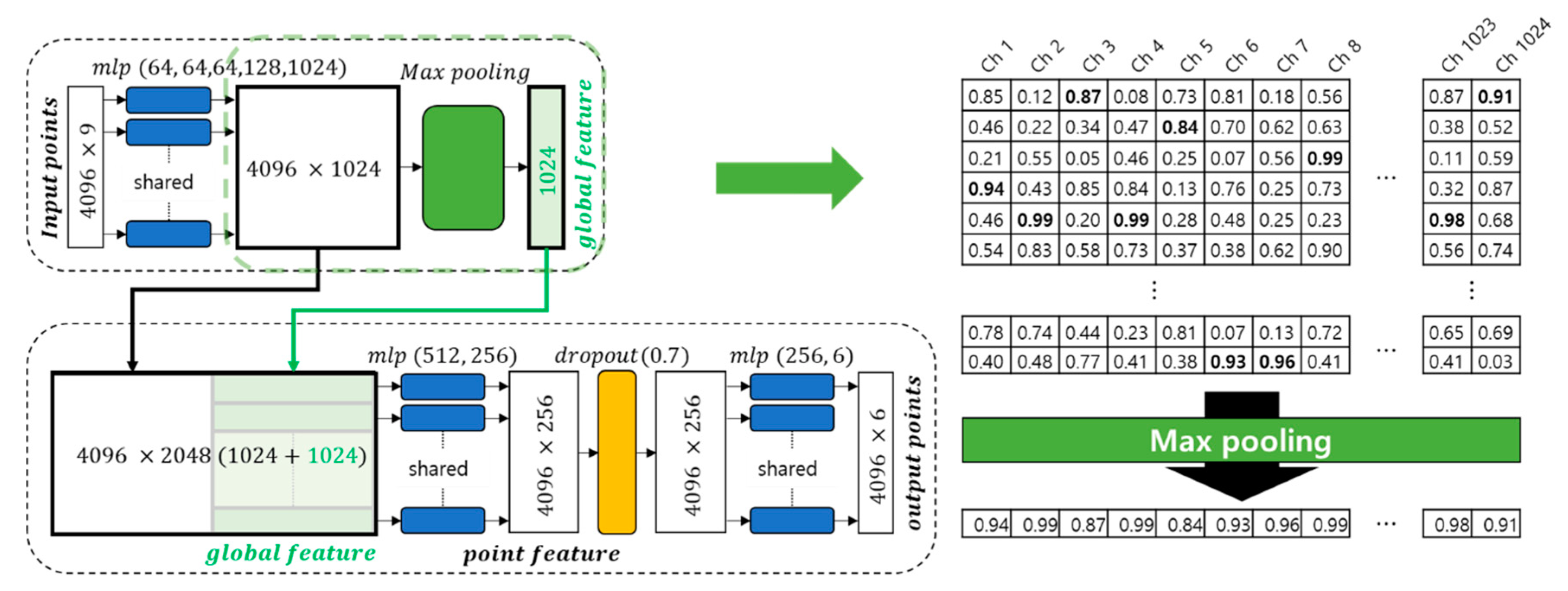
Figure 1. Max-pooling in the semantic segmentation network of PointNet.
Remotesensing 12 03757 g001
Figure 2. (a) Hierarchical convolution on regular grids and (b) point clouds.
Remotesensing 12 03757 g002
Figure 3. The (a) dynamic graph, (b) edge features, and (c) semantic segmentation network of Dynamic Graph Convolutional Neural Network (DGCNN).
Remotesensing 12 03757 g003
Figure 4. Partitioning of blocks from bridge point clouds.
Remotesensing 12 03757 g004
Figure 5. 3D reconstruction of full-scale bridges.
Remotesensing 12 03757 g005
Figure 6. Overlap ratio of the block partitions (75%).
Remotesensing 12 03757 g006
Figure 7. Segmentation results for (a) bridge 3–1 and (b) bridge 2–1.
Remotesensing 12 03757 g007
Table 1. Dimensions of the bridges.
BridgeLengths of the Piers along the Longitudinal Direction (m)Width (m)Length (m)
Bridge140.0035.73282.23
Bridge210.0041.4267.28
Bridge37.0029.6587.45
Table 2. Folds for the data.
FoldTrainValidation
1Bridge 1–2, Bridge 2–1, Bridge 2–2, Bridge 3–1Bridge 1–1, Bridge 3–2
2Bridge 1–1, Bridge 1–2, Bridge 2–2, Bridge 3–2Bridge 2–1, Bridge 3–1
3Bridge 1–2, Bridge 2–1, Bridge 2–2, Bridge 3–1Bridge 1–2, Bridge 2–2
Table 3. Hyperparameter tuning for the three models.
ModelHyperparameterValue
PointNetEpoch60
Batch size36
Learning rate0.001
PointCNNEpoch60
Batch size8
Learning rate0.001
DGCNNEpoch60
Batch size12
Learning rate0.001
Table 4. Performance comparison of the semantic segmentation models according to block parameter variation.
Block Size50%66%75%80%
PointNet
3 m70.09%79.99%88.96%93.83%
6 m65.65%67.17%69.48%68.31%
9 m60.30%64.46%63.41%65.60%
12 m61.14%59.68%62.32%64.89%
15 m58.25%56.51%55.42%61.22%
DGCNN
3 m84.69%89.67%93.44%94.49%
6 m69.58%76.36%75.62%87.03%
9 m54.73%64.12%74.12%69.53%
12 m55.08%59.33%61.97%63.00%
15 m58.16%63.10%52.47%59.41%
PointCNN
3 m91.25%89.57%91.04%91.39%
6 m92.55%91.58%91.94%92.00%
9 m91.14%91.07%90.49%91.23%
12 m89.79%91.41%91.12%90.71%
15 m90.64%90.85%91.14%90.19%
Table 5. Segmentation results for the bridges in the cross-validation for each class.
IoUPointNetPointCNNDGCNN
Abutment55.47%30.87%73.78%
Slab97.90%95.69%96.39%
Pier92.22%75.45%79.11%
Girder90.96%92.18%91.71%
Surface80.59%78.45%88.38%
Background88.62%88.06%91.74%
Mean IoU84.29%76.78%86.85%
Publisher’s Note: MDPI stays neutral with regard to jurisdictional claims in published maps and institutional affiliations.