1. Introduction
Optical satellite remote sensing images have been applied on varied applications. To better exploit these images and improve image resolution, researchers have turned their attention to super resolution reconstruction (SRR) methods, which turn low-resolution (LR) images into high-resolution (HR) ones. To simplify expression and clarify the distinction from HR images, the results predicted by SRR methods from LR images are called super resolution (SR) images.
In that SRR task exists an ill-posed problem [
1]: the methods for this task must spare no effort to exploit prior knowledge. Some methods take prior knowledge by establishing degradation models [
2], some others are based on sparse representation and learn a dictionary for transforming between LR patches and HR patches [
3,
4]. However, the lack of learning ability limits the performance of these methods. Therefore, Dong et al. introduced a convolutional neural network (CNN) of high learning ability into SRR tasks and proposes the SRCNN [
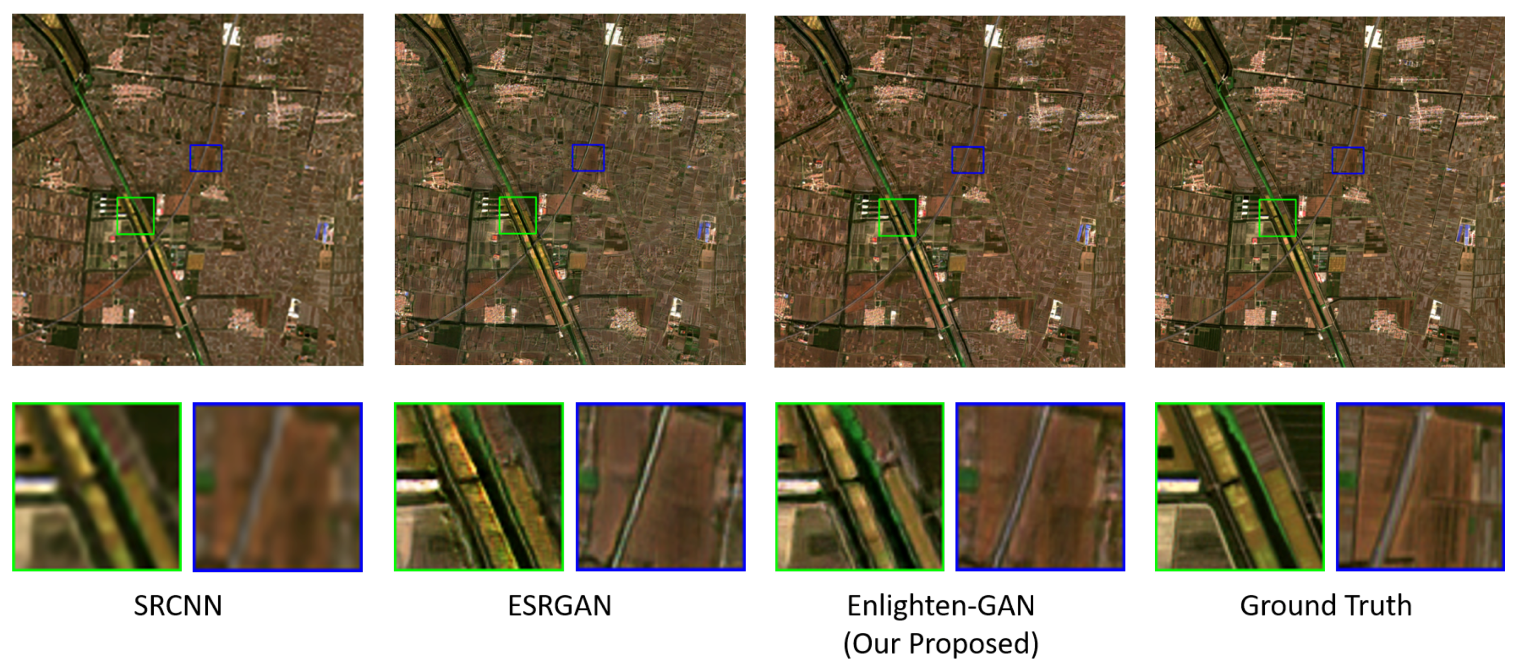
5]. However, this method adopts pixel loss to optimize network, and leads to overly smooth results as pixel loss does not take perceptual quality into account, as shown in the first column of
Figure 1. Despite the usage of residual learning [
6,
7,
8], recursive learning [
9], dense connection [
10,
11], attention mechanism [
8,
12], and deep learning architectures to boost performance, the results from pixel-loss-based methods still suffer from the aforementioned issue. Thus, Johnson et al. adopted the perceptual loss to measure semantic similarity [
13]. Sajjadi et al. adopted texture loss focusing on gradient similarity defined with Gram matrix [
14]. Their results surpass the previous ones, but are still of obvious margin compared with real HR images.
Generative adversarial networks (GANs) have been proved to be effective for generating realistic images thanks to the adversarial loss. Ledig et al. first utilized GAN for SRR task and designed the SRGAN [
1,
15]. Subsequently, ESRGAN improved it with Residual-in-Residual Dense Block (RRDB), relativistic discriminative loss, and perceptual loss without activation [
16]. The results from GAN-based methods are realistic and satisfying applied on natural images.
Remote sensing images have huge viewport and variable scene, posing challenges to SRR tasks. As shown in the left patch in the second column of
Figure 1, ESRGAN produces artifacts such as the unpleasing yellow line at the right end of the field in the left patch and the white road in the right patch, which is actually gray. Variable scenes and complicated environment in mid-resolution remote sensing images exceedingly affect their judgment. Orienting to remote sensing images, Lei et al. proposed the LGCNet, with a skip connection structure similar to Kim et al.’s work [
17]. Moreover, Jiang et al. designed the EEGAN to purify the high-frequency map and suppress image noise [
18]. Nevertheless, these networks are trained and tested on sub-meter resolution images, which is of clear object contour. Currently, there is no SRR method designed for mid-resolution images.
There is another distinctive issue in remote sensing images in that remote sensing images are highly variable, while the networks can only process small size images limited by memory. In most deep learning applications, the image is cropped into patches and processed separately. Afterwards, these patches are merged into a whole. However, a casual merging strategy leaves a seam line between adjacent patches in the predicted images.
According to the aforementioned issues, in this paper, we propose an SRR method called Enlighten-GAN that primarily focuses on mid-resolution remote sensing images. The Enlighten-GAN struggles to induce network converging to a stable and reliable point by varied means. Our main contributions are listed below.
We design a novel Enlighten-GAN with an enlighten block. The enlighten block benefits the network by setting an easier target to ensure it receives effective gradient. Owing to the varied scale reconstructed results, the enlighten block gains even higher generalization ability. Our proposed Enlighten-GAN proves itself in our comparison experiments on Sentinel-2 images, exceeding the state-of-the-art methods.
We introduce and employ a Self-Supervised Hierarchical Perceptual Loss for training rather than the conventional perceptual loss defined with VGGNet [
15], which is more suitable for SRR-like tasks. We conduct ablation experiment to verify its effectiveness.
To address the merging issue, we propose a clipping-and-merging method with a learning-based batch internal inconsistency loss, by which the seam lines in the predicted large-scale remote sensing images are dismissed.
The remainder of our paper is organized as follows. In
Section 2, we overview the previous SRR methods and GAN variants, for better demonstrating the idea of our paper. In
Section 3, we introduce how our proposed Enlighten-GAN works and improves performance.
Section 4 validates the utility of our works, followed by
Section 5 which concludes our study.
3. Methodology
The SRR methods aim to turn a H × W pixel image into
sH ×
sW, where
s refers to the upsampling scale. We set
s to 4 like most methods do [
1,
5,
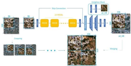
16] to ensure the fairness of the performance comparison. Due to the limitation of memory, we crop the given images with overlaps between patches, predict the SR outputs with our GAN network, and eventually merge them carefully at original position into a whole. To take a closer look at our method, we further discuss our network architecture, loss function, and image merging strategy in the followings.
3.1. Enlighten-Gan
ESRGAN outperforms the other SRR methods when applied on natural images [
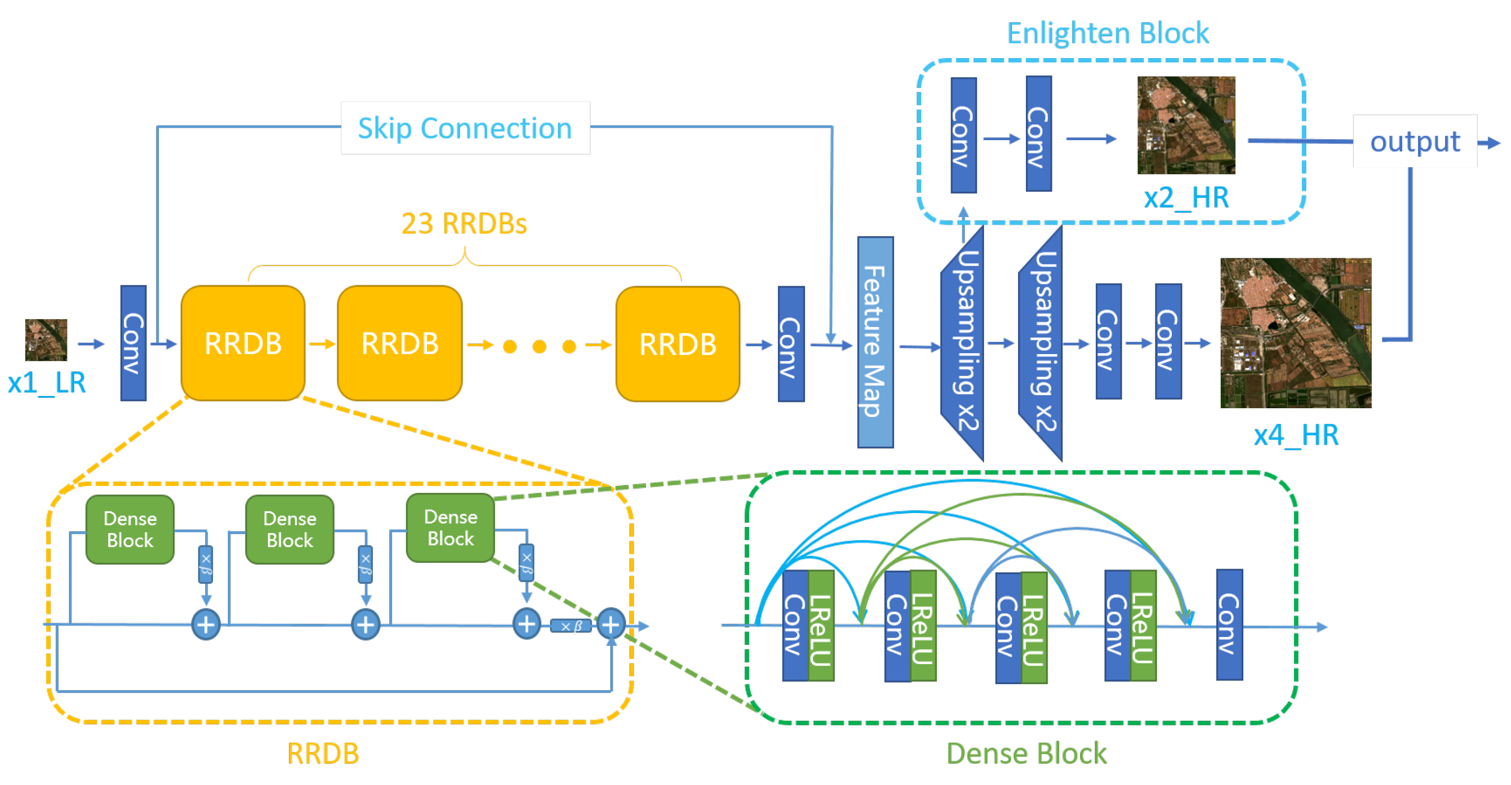
16]. Therefore, we take it as our baseline network when designing the Enlighten-GAN. We modified it with the enlighten block and the 1-Lipschitz metrics for stable results in the remote sensing images SRR task. The proposed Enlighten GAN consists of a generative model as shown in
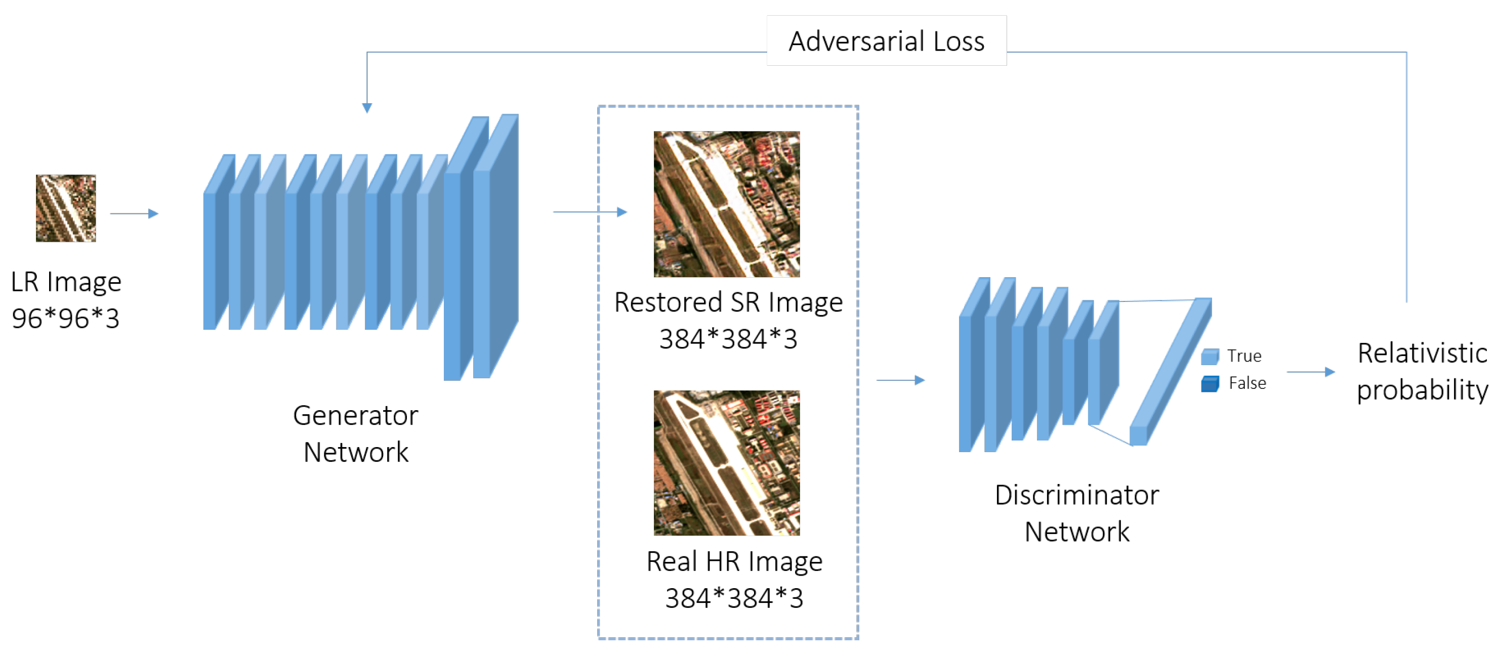
Figure 3 and a discriminative model as shown in
Figure 4.
The generative model adopts an LR image as input and attains both a 2-times and 4-times HR image as output. After one convolutional layer, 23 basic units named Residual-in-Residual Dense Block (RRDB) are arranged to recursively learn the detail from images. Each RRDB contains three dense blocks with densely skipping connections and no batch normalization. Subsequently, a skip connection extracts the features from high- and low-level layers into a feature map, based on the idea of residual learning [
7]. So far, we employed a similar structure to the ESRGAN to extract high-dimension feature maps. We apply this feature map to predict SR images by nearest neighbor interpolation and convolution operation. Besides 4-times outputs, we propose the enlighten block to produce 2-times upsampling results as an easier target. This block enables the feature maps obtained from skip connection to receive a meaningful gradient and learn high-frequency information at an easier and a harder mode alternatively. It prioritizes the network to have more generalization ability owing to its multi-output structure. Thus, the generated HR images from the G are realistic and natural.
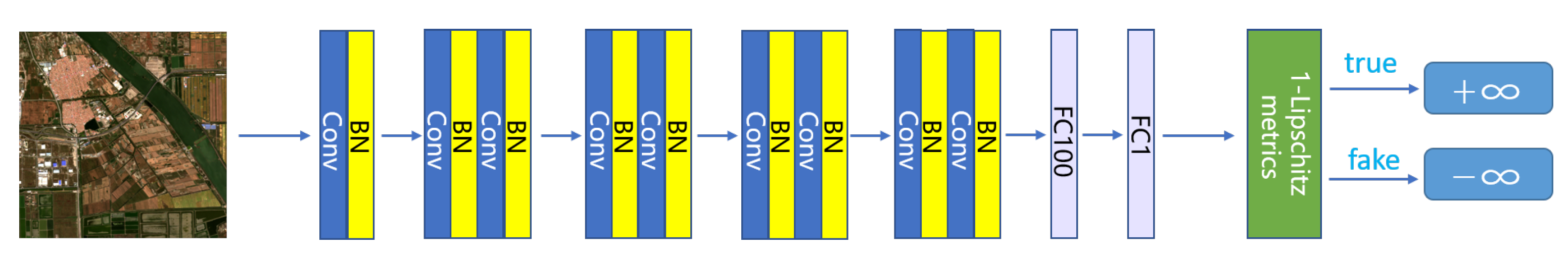
The discriminative model distinguishes the image between true or fake, provides the adversarial loss for generative network, and thus promotes the quality of generated images. The architecture of the D is brief yet effective. Both synthesized images from the G and real-world images are fed into this network. Inspired by VGGNet, the pipeline involves sequential convolutional and batch normalization layers, ending with a fully connected layer to predict the possibility of the given image being true. To pursue a stable convergence, we adopted non-activated 1-Lipschitz metrics
f as output rather than directly predicting possibility, inspired by WGAN [
20]. This modification guides the real-world sample to contribute gradient to our networks, and thus attains a better performance. Notably, when calculating adversarial loss, we focus on the optimization of the 4-times result rather than both results, so that only one discriminative network needs to be trained. The more details of architecture are shown in
Figure 4.
3.2. Model Optimization
To optimize our designed models, we collected sets of mid-resolution remote sensing images, and downsampled them by 4 times to obtain the LR and HR image pairs as training and validation datasets. The loss function for optimizing our network consists of generative and discriminative loss.
As there are two SR images as result, denoted as
I and
I, we should separately optimize them, and thus form our generative loss function as follows:
where
Loss and
Loss represent pixel loss and perceptual loss, respectively. The pixel loss is defined as the L2-distance between the ground truth and fake images, while perceptual loss parameterized by
refers to the distance calculated by feature maps of them. Though some found that the L2-distance pixel loss tends to neglect slight differences and thus lead networks to produce blurred yet safe results in CNN networks [
26], we observed that it performed well in the GAN structure with the supplement of adversarial loss and perceptual loss. Notably, the loss for the 2-times output part is parameterized by
to balance the weight between multi-outputs. Our generative loss function ends with the adversarial loss,
Loss parameterized by
. It refers to 1-Lipschitz metrics
f predicted by the D and encourages the G to produce more misleading thus better results. Experiments show the Wasserstein loss predicted by 1-Lipschitz metrics conducts a stable training procedure.
As seen from Equation (
1), the perceptual loss item requires effective feature maps to describe the semantic information of images. Previous methods adopted outputs of the layer before fully connected layer in the VGGNet pretrained on ImageNet [
16]. However, when validating this idea on remote sensing images, we found networks trained without perceptual loss get a better performance, unexpectedly. We attribute it to applying a classification model to predict feature maps on SRR task. As matter of a fact, classification models tend to attach attention to high-level features rather than pixel-level details. Further, the pooling layers in the VGGNet discard high-frequency information the SRR methods recovered, which is exactly the divergence between SR images and HR images. These factors affect the effectiveness of predicted feature maps. Thus, we proposed the Self-Supervised Hierarchical Perceptual Loss, which employs an autoencoder network instead of a classification model to predict feature maps. The autoencoder aims to recover itself from feature maps [
31]. Theoretically, the predicted feature maps retain all details from images in order to recover themselves, and thus can be implied to be more reliable.
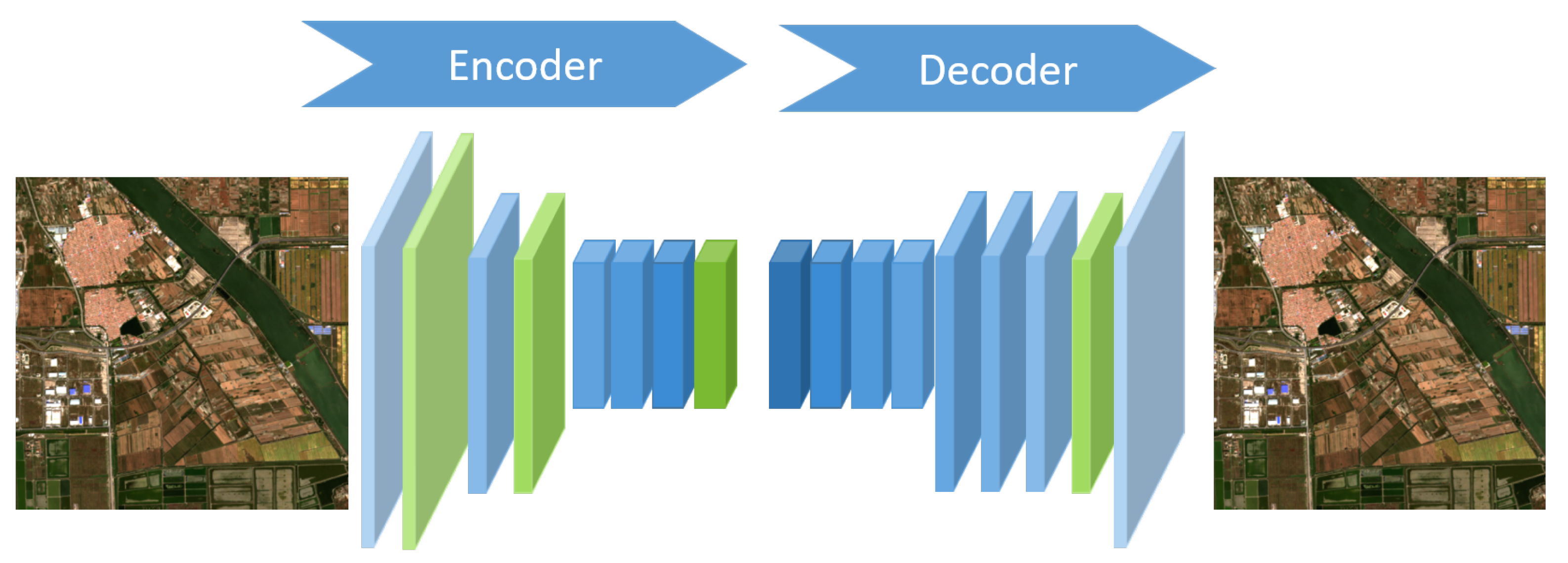
We build and train a novel and brief autoencoder, constructed by the convolutional layers and the ReLU layers without batch normalization layer. The autoencoder consists of an encoder and a decoder. The encoder pools the inputs into small size and high-dimension feature maps by nearest neighbor interpolation. Using bilinear interpolation, the decoder recovers feature maps back to images the same as the input. The reconstructed output of the autoencoder is supposed to as similar to the inputs as possible. The whole architecture of autoencoder is shown in
Figure 5.
Though we replace the max-pooling layer, which partly discards location information, the autoencoder network still retains a pooling layer for thrift memory occupation. Therefore, we summarize features from varied layers to compose a perceptual loss hierarchically. Specifically, we select the features of layers 3, 8, 17, 34 in our autoencoder, which have been marked in green as perceptual features. This assures the proposed perceptual loss to contain both semantic and pixel-level information. As the variance of each feature map should describe the discrepancy between images as opposed to layers, we normalize the deviation of perceptual feature from each layer to 1 and sum their corresponding perceptual loss up.
As for the optimization of D, we expect it to correctly distinguish between real and fake data. Furthermore, due to the diversity of samples, the weights of the G change significantly due to its high gradient, so we take the advantages of a gradient penalty [
20] to avoid a complete change in one batch, and formed the discriminative loss as follows:
where the
Loss refers to predicted 1-Lipschitz metrics
f when the sample is fake, and the
Loss refers to the otherwise situations. The last item refers to the gradient penalty, where the
g refers to the gradient flow of each weight parameter for loss function. In summary, each image pair contributes gradient by generative and discriminative loss function aforementioned. However, considering patches merging issue, there should be a further batch inconsistency loss to improve performance, which is discussed in following sections.
3.3. Patches Clipping-And-Merging Method
As deep learning networks can only accept small size images limited by memory, we crop images into patches to fit the network more often than not. To ensure the seam line between patches is natural and realistic, we crop patches with overlaps as most remote sensing deep learning applications do. The predicted SR patches should pose in their original area to compose the entire SR image, which brings diversity on how to address pixel value in overlaps. The high-level semantic tasks choose to take the average value of each patch. However, the average operation influences the clarity of images, against the purpose of improving image quality. On the other hand, as the overlap involves information from two patches, there is pixel value discontinuity between the overlapping and non-overlapping areas. These two phenomena get even worse when the overlaps of adjacent patches go more inconsistent, and get disappear as they come to the same. As long as the difference exists, roughly changing the overlapping rate or merging them in a weighted way cannot solve them both.
Thus, we design the clipping-and-merging method with the batch internal inconsistency loss to handle large-scale remote sensing images. First, as we found the patches inconsistency is source for image stitching problem, we encourage network to produce batch consistent results. We take 25% as the overlapping rate, as empirically we found it guides the two adjacent patches to getting similar receptive fields in the overlaps. Specifically, we crop the 168 × 168 sized images into 2 × 2 parts, namely, 96 × 96 sized patches, forming four overlaps of 24 pixels. We process these 4 patches as a batch into networks. Furthermore, we introduce the inconsistency loss, and thus the generative loss for this batch comes to
where the
Loss refers to Equation (
1), to measure the distance between SR images and HR images. The inconsistency loss,
Loss, represents the L2 distance in each overlap between patches and is parameterized with
. This loss urges the network to predict similar results based on similar receptive fields as we designed.
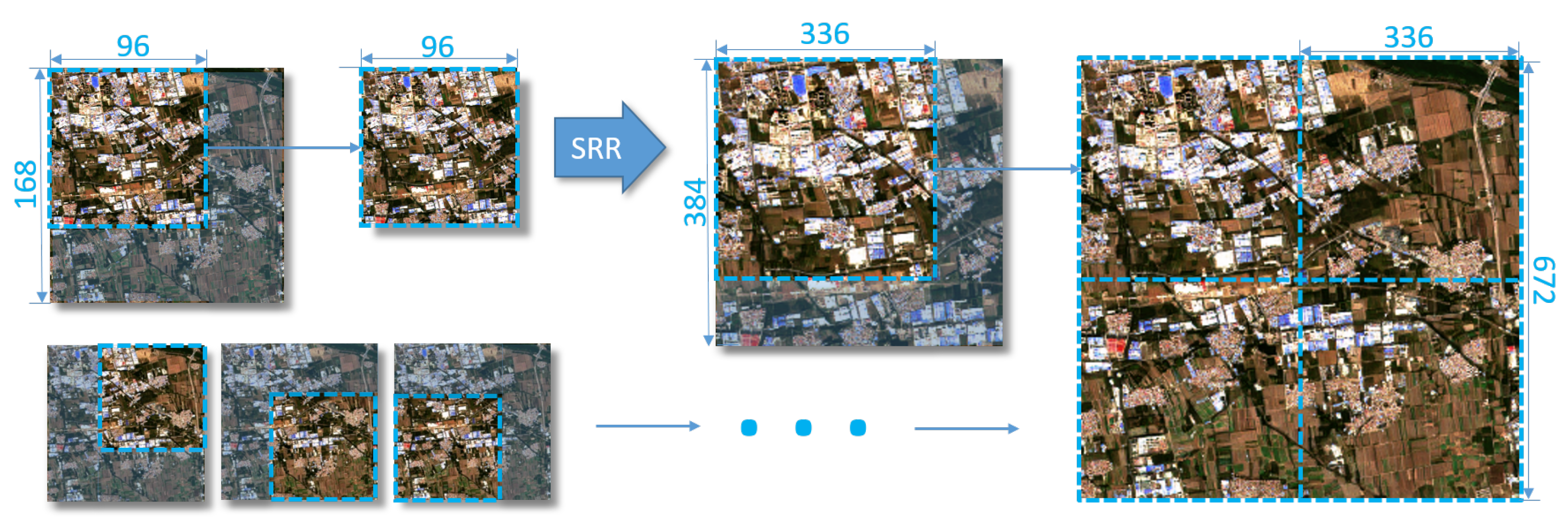
To completely dismiss the risk of blurred phenomena from average operation, we adopt the clipping-and-merging method to predict large-scale remote sensing images. We crop the images into patches with overlaps as mentioned above, restore SR patches separately, and clip these patches before merging until no overlap left, as shown in
Figure 6. Specifically, the out-half side of overlap in each cropped patch is clipped and discarded, while the inside and reliable half is retained. The overlap in the predicted result is composed from two neighbor patches half by half. Experiments show that images predicted by our method leave no visual seam line.
4. Experiment
Based on the structure mentioned above, we conduct experiments with the Enlighten-GAN on mid-resolution remote sensing images. Concrete implementation details and experiment results are discussed in this section.
4.1. Implement Details
The experimental dataset is generated from Sentinel-2 images. Sentinel-2 is a mid-resolution imaging satellite carrying a multispectral imager for land monitoring. It can provide images of vegetation, soil and water cover, inland waterways, and coastal areas, as well as emergency rescue services. Sentinel-2 takes multispectral images at a height of 786 km, covering 13 spectral bands and a width of 290 km. We select bands 2, 3, and 4, representing blue, green, red bands, respectively, of 10-meter resolution to generate images for training and testing.
Thus, we train our model on two 10,980 × 10,980 size RGB images with rich texture and details information. These images are cropped into 423 images in size of 672 × 672 pixels. Among these images, we split them into 323 images for training and 100 images for testing. Those images are downsampled by 4 times to 168 × 168 pixels, and thus constitute the LR and HR image pairs. As mentioned before, we applied the cropping-and-clipping method to crop images into 4 patches with overlapping rate of 0.25, namely, 96 × 96 pixels patches as the same with the input size of the G, and feed them into networks as a batch. When testing, we directly feed the 168 × 168 size images into network and attain the SR images, since the testing procedure costs less memory occupation than training does. Moreover, we took advantages of data augmentation operations online on the dataset for the generalizability of model, such as 90-degree rotation randomly several times.
Before training the Enlighten-GAN, we prepared the autoencoder in advance for the calculation of Self-Supervised Hierarchical Perceptual Loss. We trained the autoencoder for 200 epochs on the same dataset. The learning rate is set to 1 × 10 as initial and get cosine-annealed during training.
For our proposed Enlighten-GAN, we trained the G for 3 epochs with
,
equal to 0, namely, only content loss remaining, to initially enable the G to produce reasonable images, forming a balance between the G and the D for a stable training procedure. Afterwards, we further train the G and the D with the
,
, and
set to 0.001, 0.006, and 0.25, respectively, in Equation (
1); the
set to 10 in Equation (
2); and the
set to 0.25 in Equation (
3) for 200 epochs. We used Adam optimizer [
32] for training with an initial learning rate of 1 × 10
. After 100 epochs, the learning rate is cut to 0.1 times of the previous value. The trained G is used for mid-resolution remote sensing SRR task, and we only retain the 4-times upsampling results.
Our method was trained and tested all on the Supercomputing Center of Wuhan University with CPUs of Intel(R) Xeon(R) E5-2640 v4 and GPUs of Nvidia Tesla V100 16 GB. The autoencoder took 17 h to be trained, while the Enlighten-GAN took 15 h.
4.2. Image Quality Assessment
Although visual quality has the final call, we still need a robust and reliable image quality assessment metric for weighing slight changes in the evaluation of SRR methods. Some previous works took Peak Signal to Noise Ratio (PSNR) as their metrics. After normalizing the images ranging from 0 to 1, The PSNR is formed as
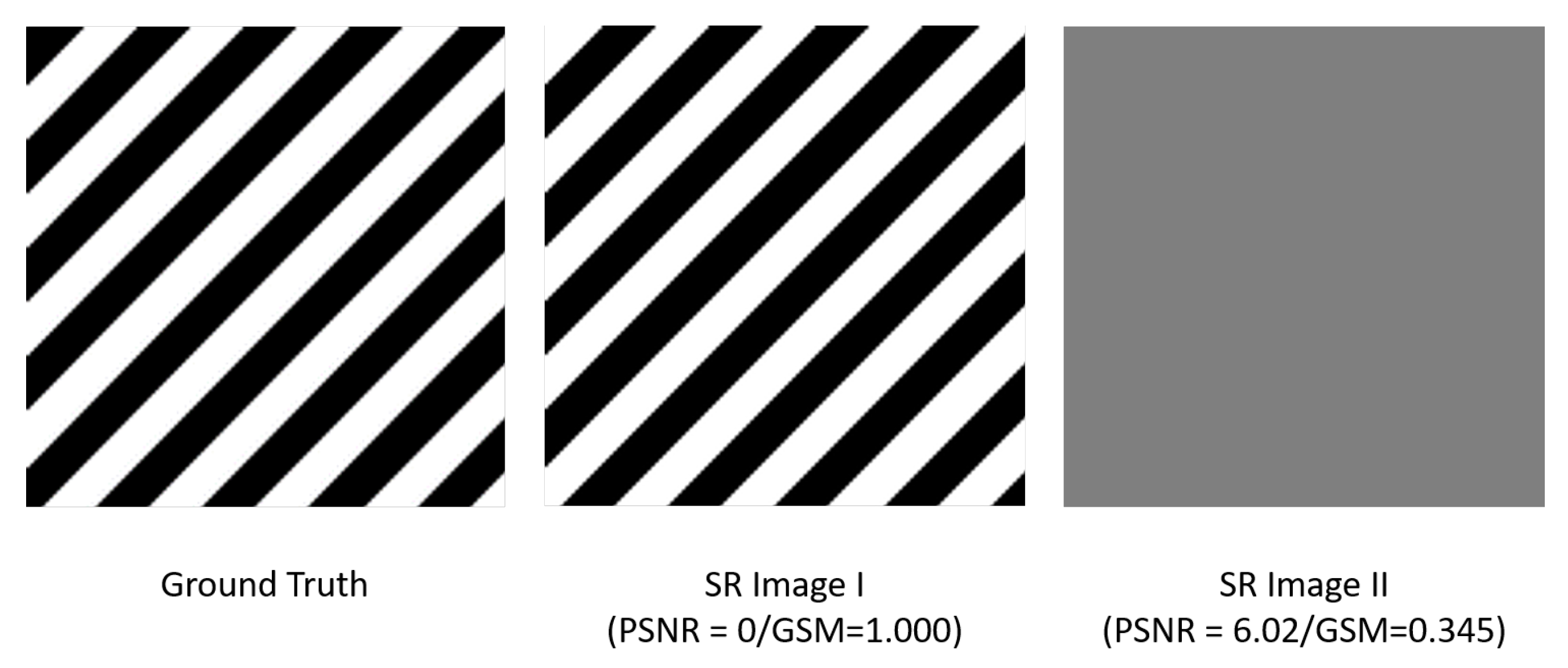
where the MSE refers to mean square error between fake images and real images. However, PSNR-orient methods, such as pixel-loss-based methods, lead to smooth results as aforementioned. Intuitively, as shown in
Figure 7, prediction with a little pixel geometry error leads to a lower PSNR, while a smooth map obtained a higher score. In ill-posed SRR methods, realistic portrait with inevitable geometry error is way meaningful than blurred outline, which implies the unreliability of PSNR.
The others choose the Perceptual Index (PI), which is also the official metric of PIRM-SR Challenge [
33]. It is a mix-up of Ma’s score [
34] and Natural Image Quality Evaluator (NIQE) [
35], which is respectively a pixel-level quality assessment and a non-reference perceptual assessment. It is formed as
where a lower PI implies a richer texture. However, the pixel-level quality is in conflict with perceptual quality [
36]. Thus, a lower PI metric does not necessarily depict higher pixel-level quality and perceptual quality at the same time. As a matter of fact, we found the results from ESRGAN with fatal artifacts attain a lower PI than ground truth in our experiment, demonstrated in the following subsection. Despite the lower PI implies richer texture, it is not assured to be real texture since the PI is a non-reference metric.
Therefore, we refer to related works and find the Gradient Similarity Metric (GSM) [
37] has a better performance in sparse coding and reconstruction channel of TID2013 [
38] in Zhang et al.’s experiment [
39]. The TID2013 dataset synthesizes varied distortion images with certain ratio and evaluates metric with that ratio. The GSM weighs the correlation coefficients of gradient, defined as
where the
g and
g refers to the gradient map of image
x and
y.
To better prove the superiority of our method, we further introduce the Learned Perceptual Image Patch Similarity (LPIPS) to measure the perceptual difference between patches [
40]. It is defined as
where
and
refer to the VGG features for layer
l, and the
refers the vector to scale the activations channel-wise. Thus, the LPIPS measures the perceptual distance between two patches with the VGG-Net. According the experiment conducted in [
40], this metric performs well in the SRR task.
To assure fairness in our experiment, we still calculate the PSNR and PI of results from SRR methods besides the GSM. Notably, a lower LPIPS, a higher PSNR, and a higher GSM imply better performance. A low PI implies an image of a high information entropy.
4.3. Results of Evaluation
We conducted evaluation experiment on our proposed method along with the input LR images and SR images from bicubic upsampling, SRCNN [
5], SRGAN [
1], ESRGAN [
16], and EEGAN [
18] methods. Thus, we obtained the result of all patches in metrics aforementioned for these SRR methods. We calculated the average and standard deviation from all patches for each method and list the quantitative results in
Table 1. For better comparison, we also list the assessment of ground-truth as reference in the table. As the CNN-based method is trained on the pixel-loss equivalent to PSNR, and thus is more likely to gain high PSNR and oversmooth result, we suppose the best score at PSNR among GAN-based methods depicts the best result. The PI closest to ground truth suggests the results are of similar information entropy to the ground truth. Notably, we suggest the GSM is the most reliable metric among them, so it has the final call. As shown in
Table 1, the Enlighten-GAN attains the best PSNR among GAN-based methods, the PI closest to ground truth, and the best GSM and LPIPS. Notably, our results get the lowest standard deviation in terms of GSM. We attribute it to our effort orienting to a stable model.
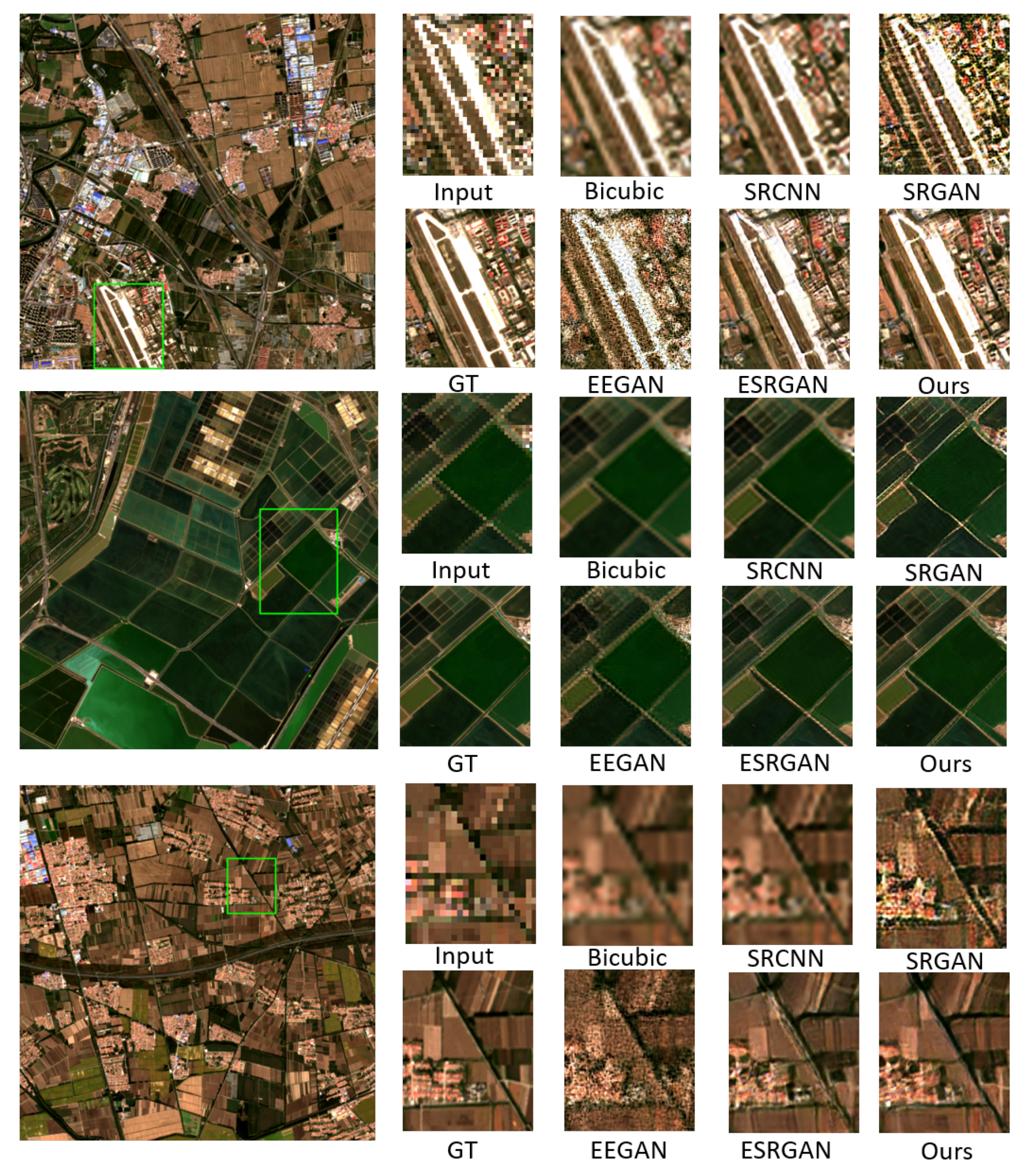
Qualitative results further depict our superiority to the other methods as shown in
Figure 8. As we mentioned in the
Section 1, the bicubic upsampling results and the SRCNN results are blurry, while the results of SRGAN are of stripped artifacts, depicted in every patch. Despite being designed for remote sensing images, the EEGAN is incompetent for mid-resolution remote sensing and produces spot artifacts. Among the state-of-the-art methods, the ESRGAN attains relative satisfying results, yet still suffers from the unstable convergence. The results from ESRGAN are of spot noise in the flattened area, such as lake and airport runway in the first and second rows. The hue of ESRGAN result does not follow the original LR patches and turns a little darker at the lake area as the second row demonstrate. ESRGAN tends to produce artifacts in the line with large color differences, such as the white line between yellow field and black road in the third row. As a contrast, the objects in our result basically retain their shapes and hues. The geometry offset in our SR images is far lower than the others, which implies the significant improvement from our methods.
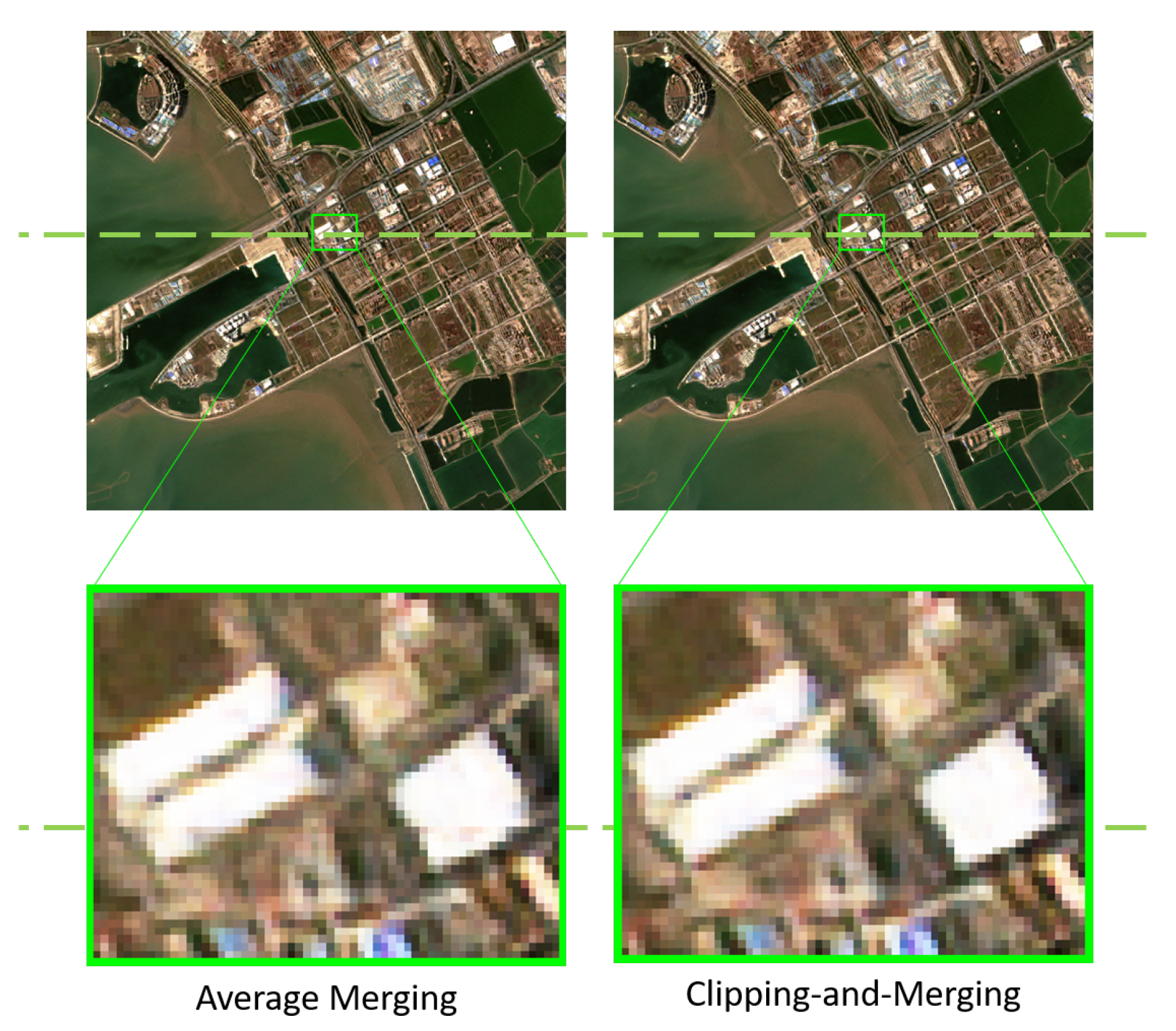
Furthermore, to assure the effectiveness of proposed clipping-and-merging method, we crop our 168 × 168 images into four 96 × 96 patches, merge them into a whole in different method, and observe the overlap, as shown in
Figure 9. The result from the clipping-and-merging method is merged without average operation, and thus is as sharp as the original patches. The common area of patches ensures the possibility for networks to predict the same outputs for adjacent patches. Therefore, the results are realistic in the overlaps. As a contrast, the result produced by averaging the two ESRGAN output patches contains an obvious seam line, cutting the building outline. In addition, the right side of the patches is blurred for average operation.
4.4. Ablation Study
To illustrate the validation of our modification and support the views we mentioned above, we list results from some of our ablation study experiments. As the slight changes may not cause obvious affect in visual, we utilize the GSM along with the PI and PSNR to carefully compare varied tricks. The overall results are listed below.
Self-Supervised Hierarchical Perceptual Loss. We found setting
to zero in Equation (
1) does not necessarily decrease the performance in ESRGAN. Therefore, we conduct an experiment to verify the effectiveness of our proposed Self-Supervised Hierarchical Perceptual Loss. We compared the model trained, respectively, with the proposed Self-Supervised Hierarchical Perceptual Loss, conventional VGGNet-based perceptual loss, and no perceptual loss. The results are shown in the
Table 2, the second row list the assessments of our results.
VGG-Perceptual attains the best LPIPS, since they both designed on VGG-Net. However, in terms of GSM, the most reliable metric we propose, it is defeated by the model trained with no perceptual loss. It stands for the uncertainty we posed in
Section 2. By contrast, our results obtain the best GSM, confirming the superiority of the Self-Supervised Hierarchical Perceptual Loss. Due to considering more on low-level features than VGG-Perceptual loss does, ours receives a slight deterioration in PI, yet it is closer to the ground-truth.
Wasserstein GAN. The main issue we face is the unstable convergence procedure. We turn to varied GAN structures for a better performance. As there is a great number of variants of GAN, we test on WGAN [
20] which has been proved to be effective and RaGAN [
24] applied in ESRGAN along with the standard GAN as baseline, to determine the best choice of our method. As shown in the
Table 3, we found the WGAN attains the most satisfying result among them, namely, the best GSM, the best PSNR, and a passable LPIPS, along with a PI close to ground-truth. Under comprehensive consideration, we apply the WGAN and its non-activation 1-Lipschitz metric in our method.
5. Discussion
From what is demonstrated in our experiments, the pixel-loss-based methods such as SRCNN attain stable SR images but suffer from the blur issue. They attain robust results with limited performance improvement. By contrast, the GAN-based methods such as SRGAN and EEGAN obtain sharp results when processing simple scene with few objects. When it comes to complicated scenes, the shallow network structures are not capable of predicting sophisticated details. Furthermore, the GAN-based methods induce the generative model to an unstable convergence, and thus product varied fatal artifacts. The artifact issue from ESRGAN is relieved, proving the effectiveness of the strategies of intensifying the network structure and stabilizing converging procedure. As shown in
Figure 8, the results of our proposed method, owing to the enlighten block and Wasserstein GAN structure, are free of artifacts and retain the correct shape and hue.
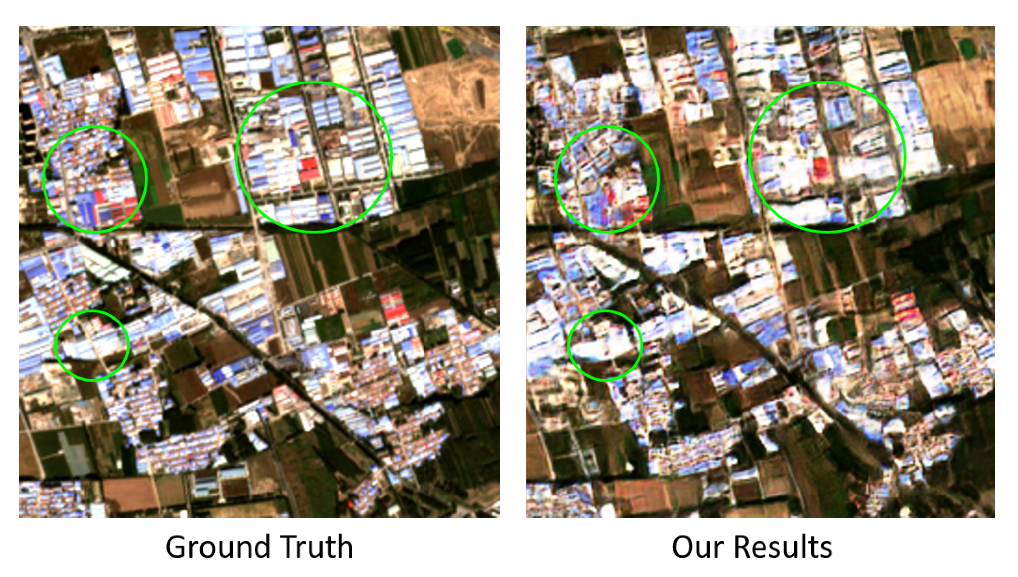
Nevertheless, there is still an obvious gap between our results and the ground-truth. Taking a closer view, the shape of objects becomes distorted and their gaps disappear, especially in the town or urban area. As shown in
Figure 10, the buildings in the edge area of town still retain their basic shape, and their corners are reliable for later application. When it goes to the central area, the networks cannot figure out the outlines of each objects from the chaotic background, especially in the area marked by green circles. Thus, the impact of surroundings and the complicated urban detail limit the performance of SRR models without external prior knowledge, even when we train on a dataset fully considering urban samples. This can be a direction to further work on.
6. Conclusions
We proposed an Enlighten-GAN method aiming at the mid-resolution optical remote sensing images SRR task. To overcome the unstable convergence, we exploit varied methods involving the enlighten block to guide the generating of feature maps, the Self-Supervised Hierarchical Perceptual Loss to optimize the Generative model, and the WGAN structure to stabilize the training process. Our experiments verify the superiority of our method. Moreover, we pioneer the merging problem for large remote sensing images. The results of images from our method turn to be realistic.
However, we found there is still a clear margin between our results and the ground-truth, especially in the urban area. The building objects are fused, and the outline of each building is unclear. In conclusion, the urban area in mid-resolution remote sensing images is an even more challenging issue to be solved in future.


 ,
, 


