
Composite Aerosol Optical Depth Mapping over Northeast Asia from GEO-LEO Satellite Observations


Abstract
:1. Introduction
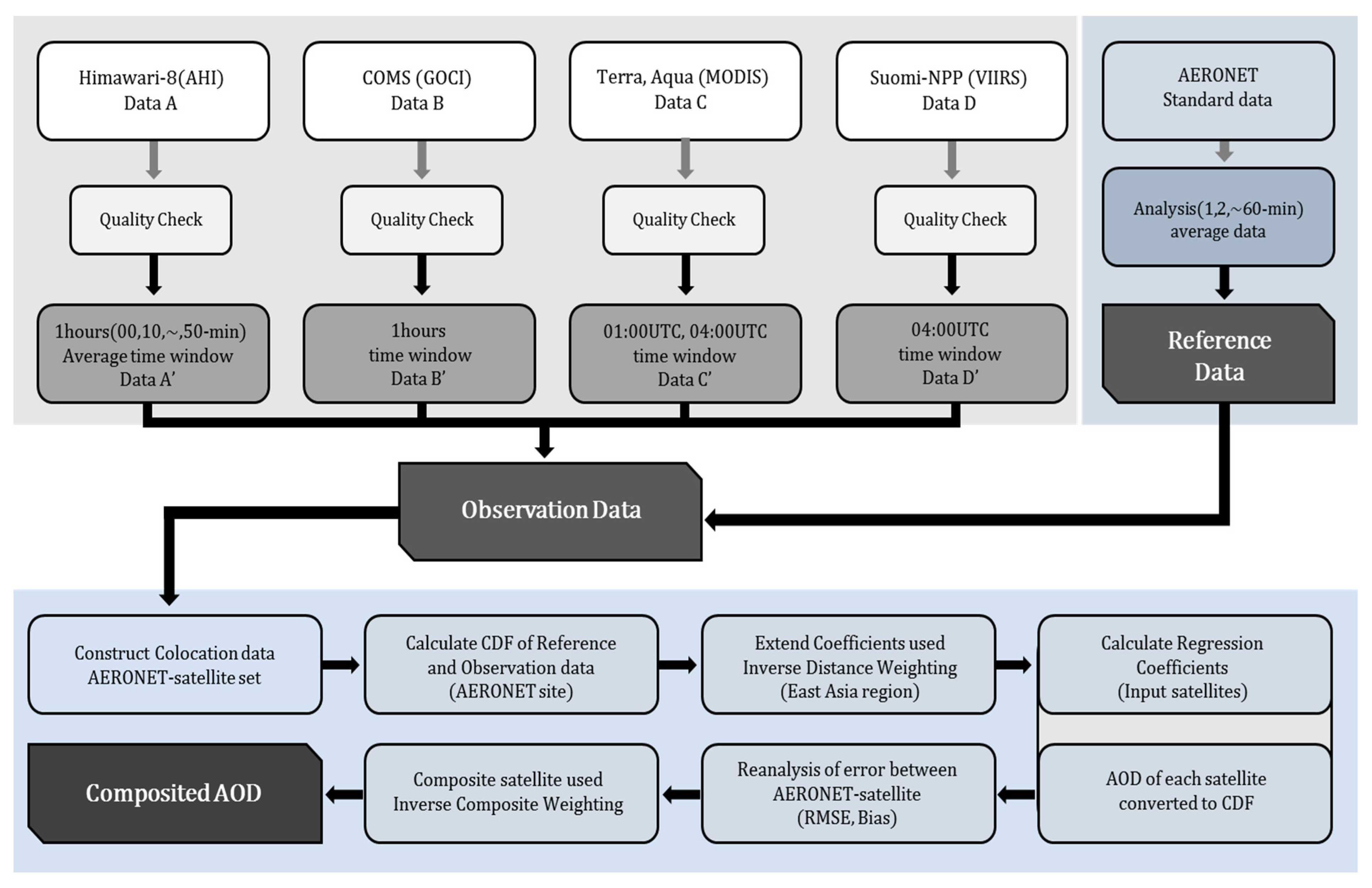
2. Data and Methods
2.1. Satellite Data
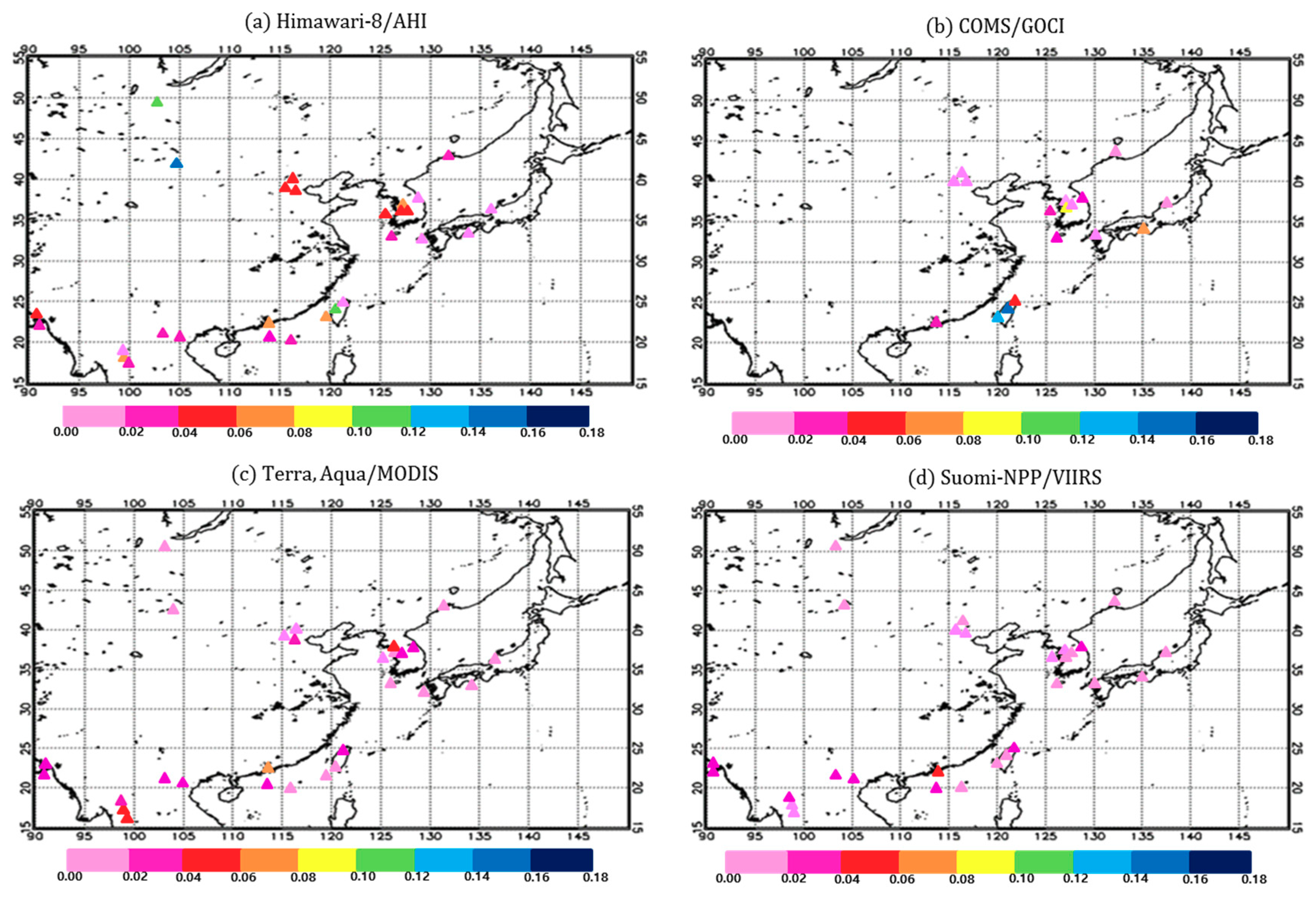
2.1.1. Himawari-8/AHI
2.1.2. COMS/GOCI
2.1.3. Terra, Aqua/MODIS
2.1.4. Suomi-NPP/VIIRS
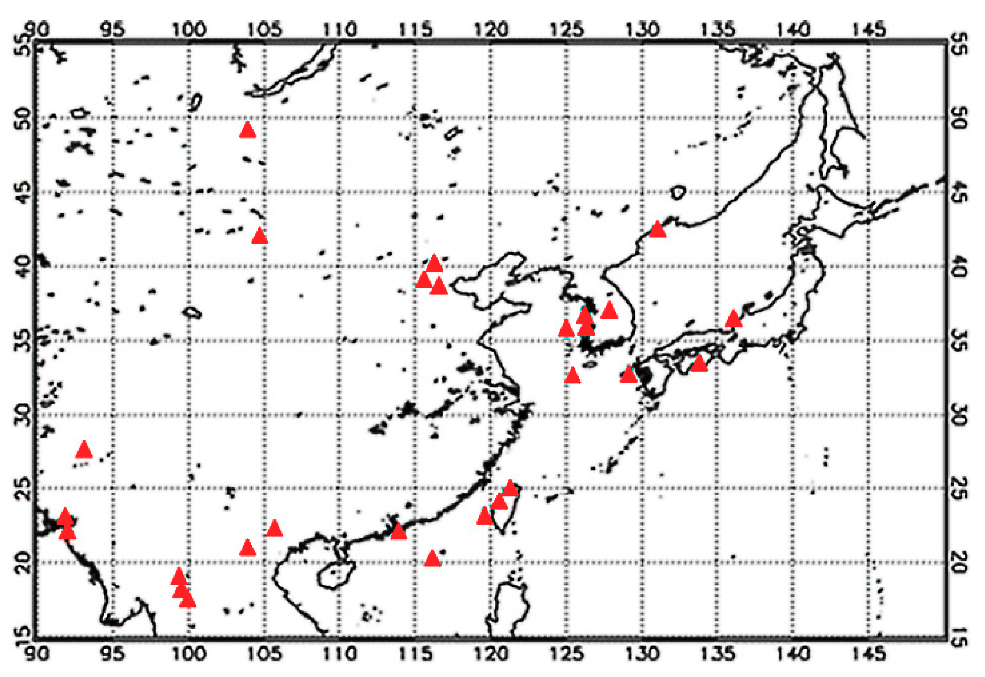
2.1.5. AERONET
2.2. Methods
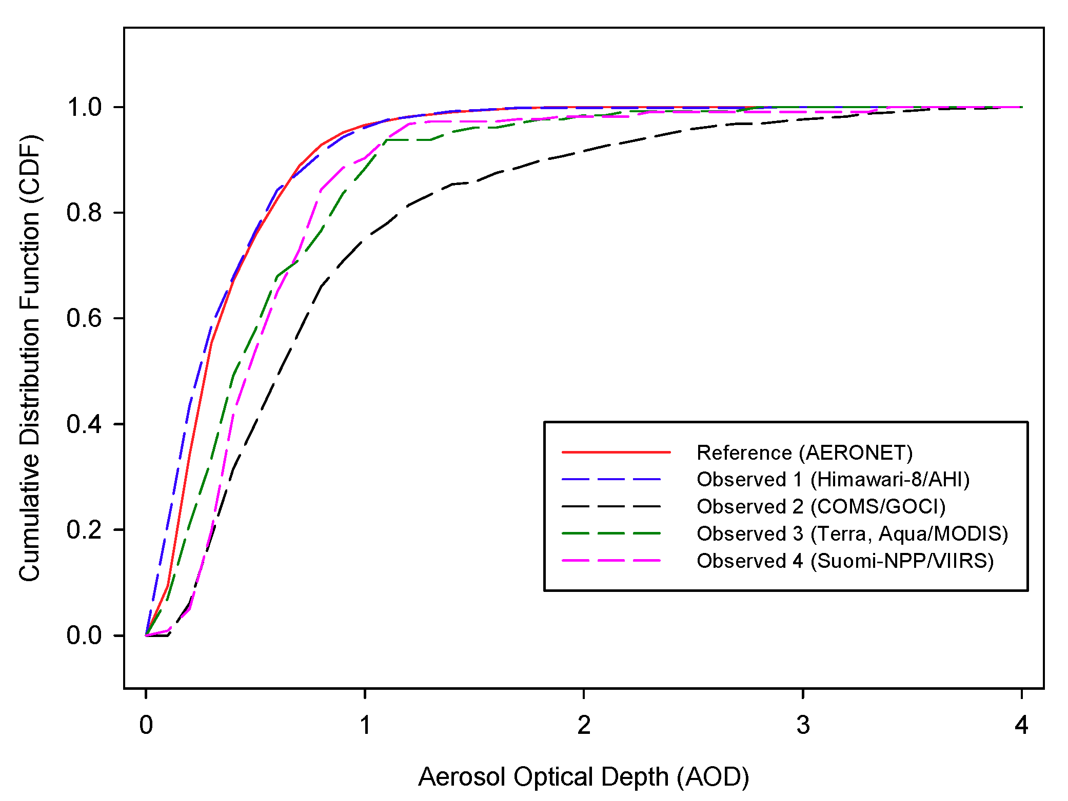
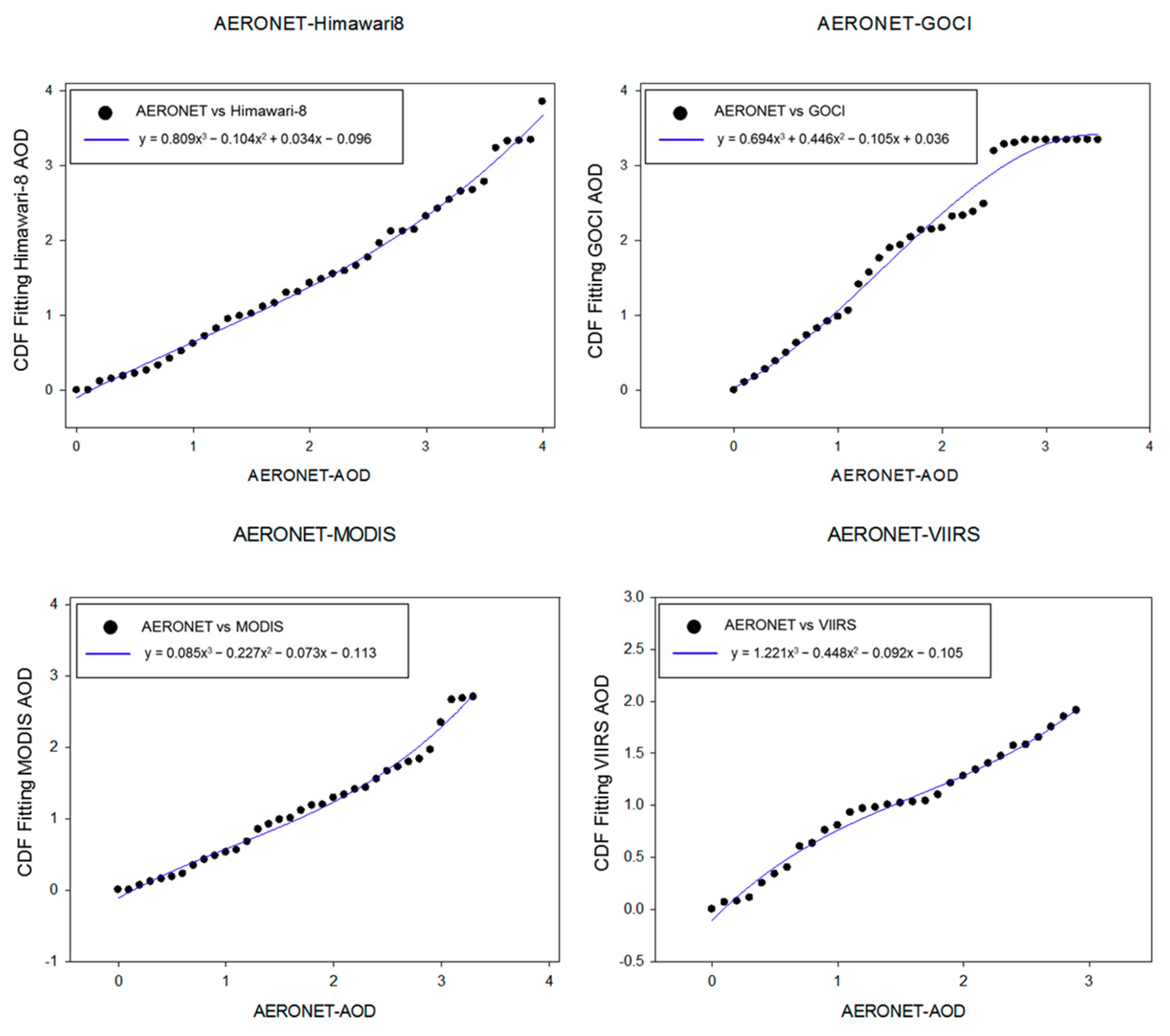
2.2.1. Cumulative Distribution Function
2.2.2. Inverse Distance Weighting (IDW)
2.2.3. Inverse Composite Weighting (ICW)
2.2.4. Composite AOD
2.2.5. HYSPLIT Trajectory
3. Results and Discussion
3.1. CDF Fitting
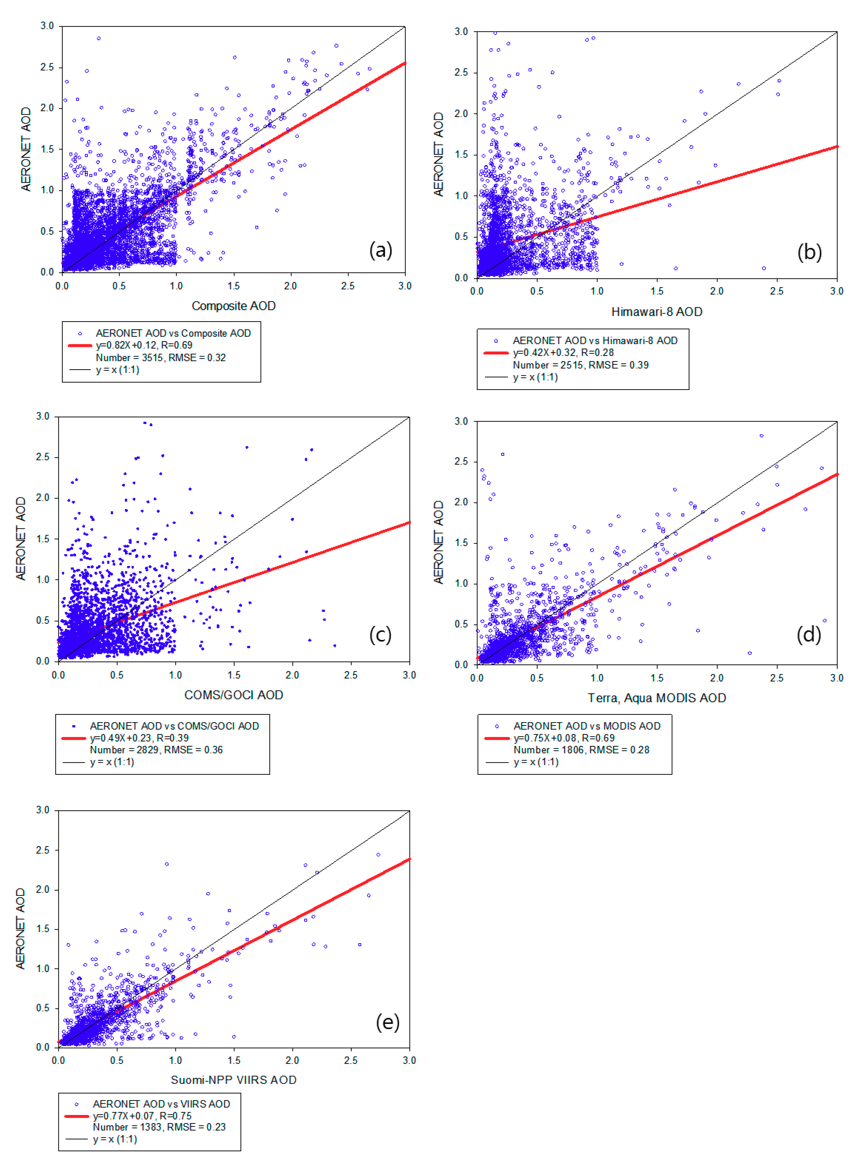
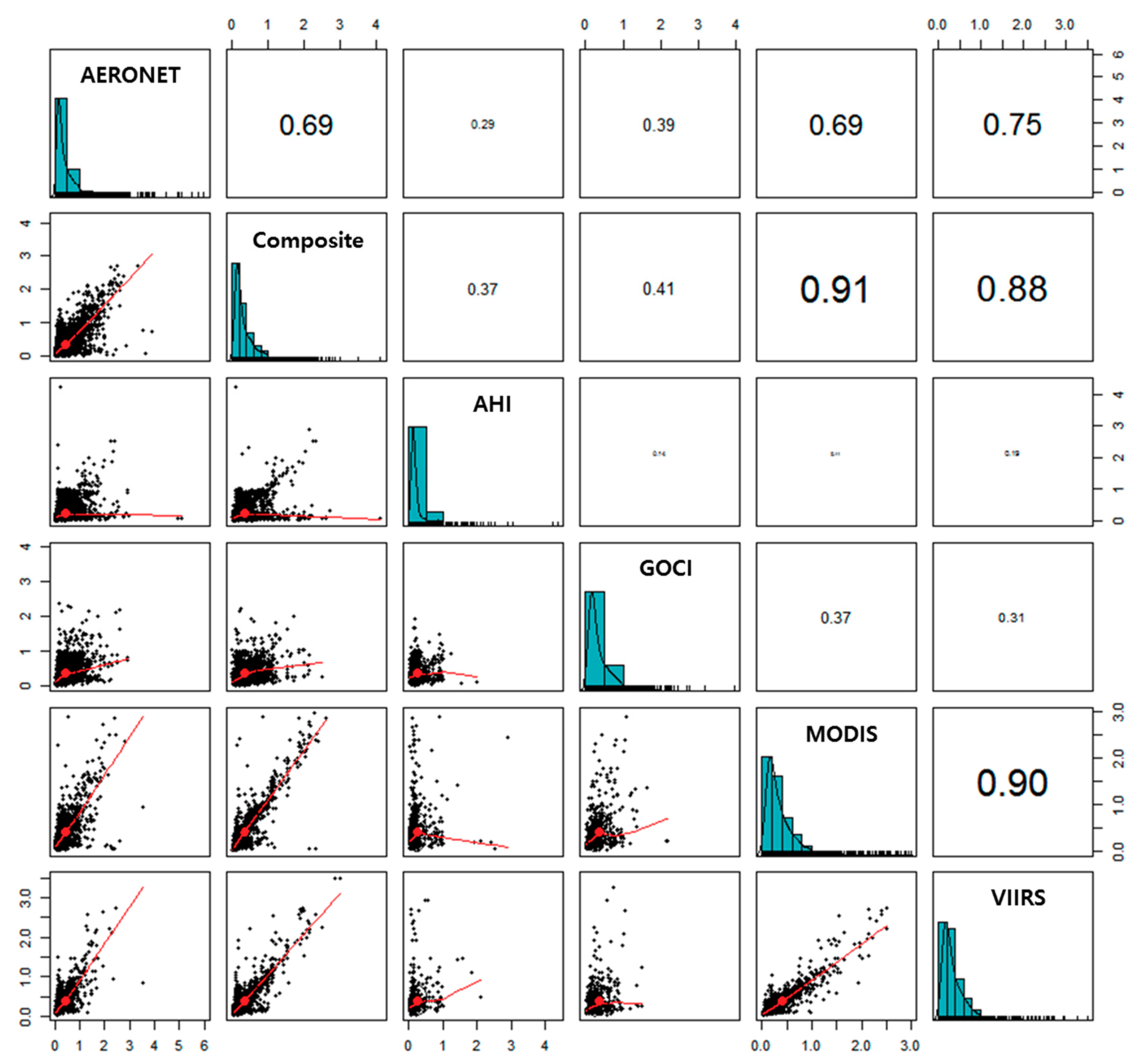
3.2. Performance of Composite AOD Products
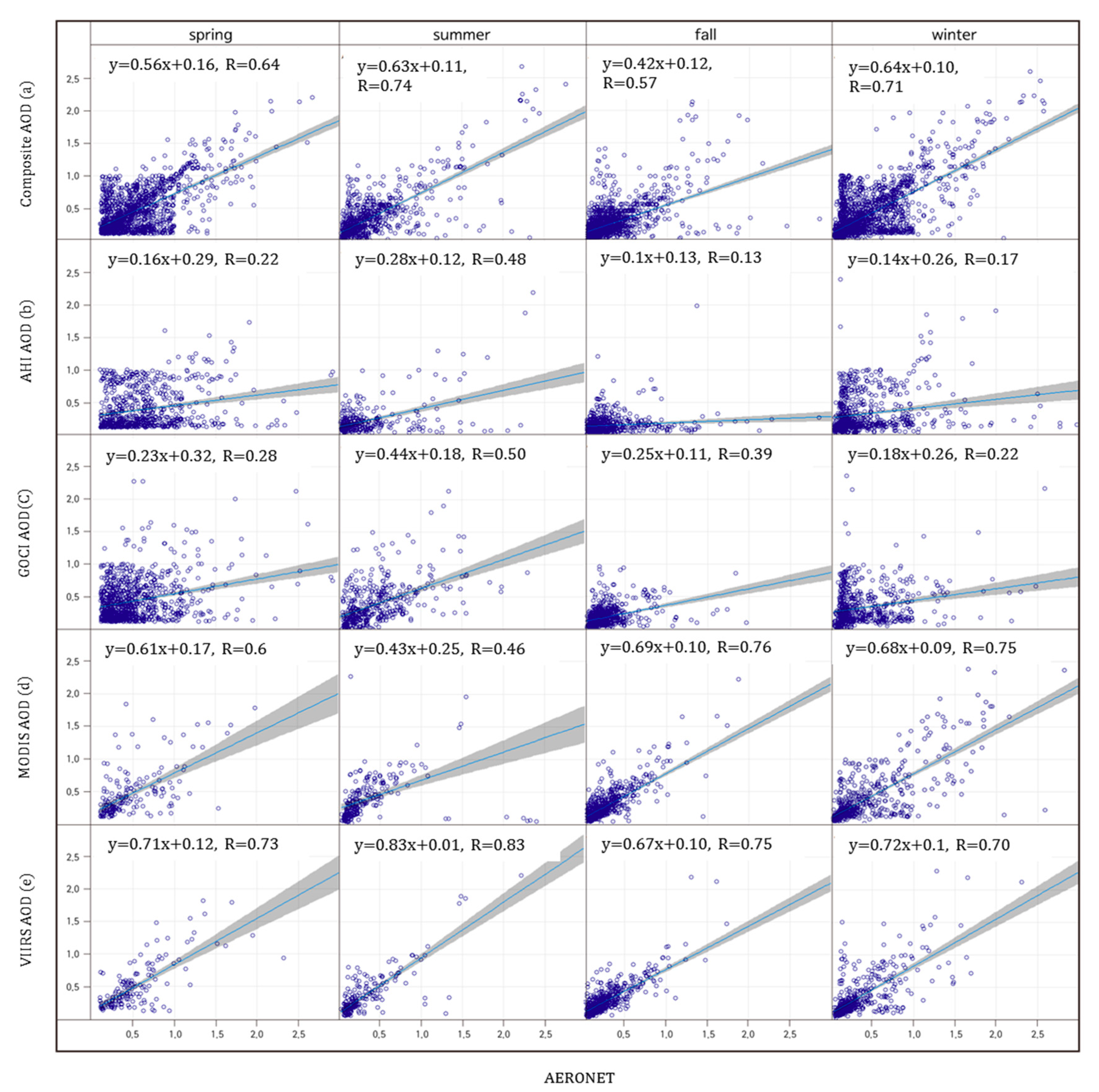
3.2.1. Composite Temporal Variability and Satellite Retrieval Accuracy
3.2.2. Composite Spatial Variability and Satellite Retrieval Accuracy
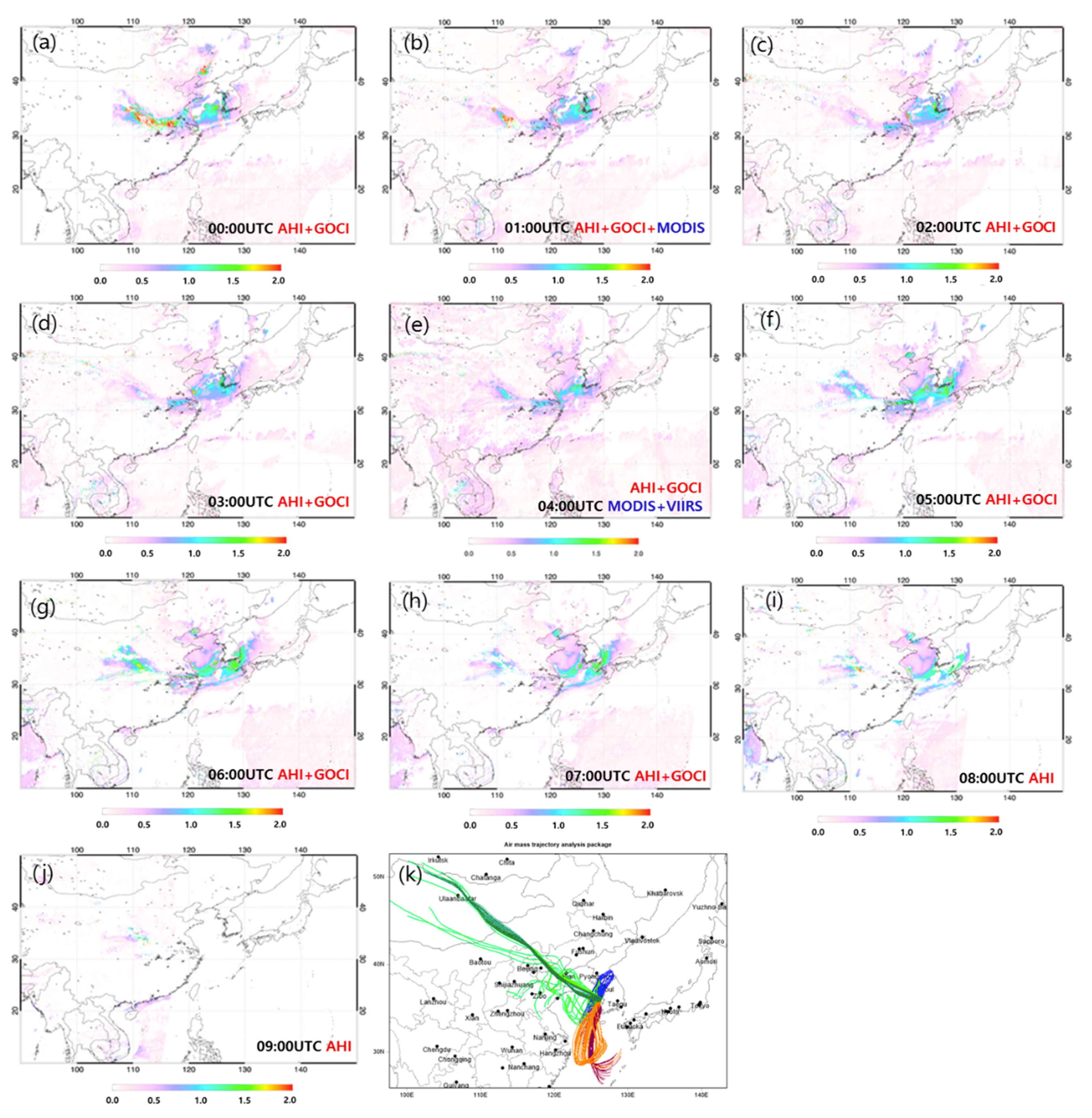
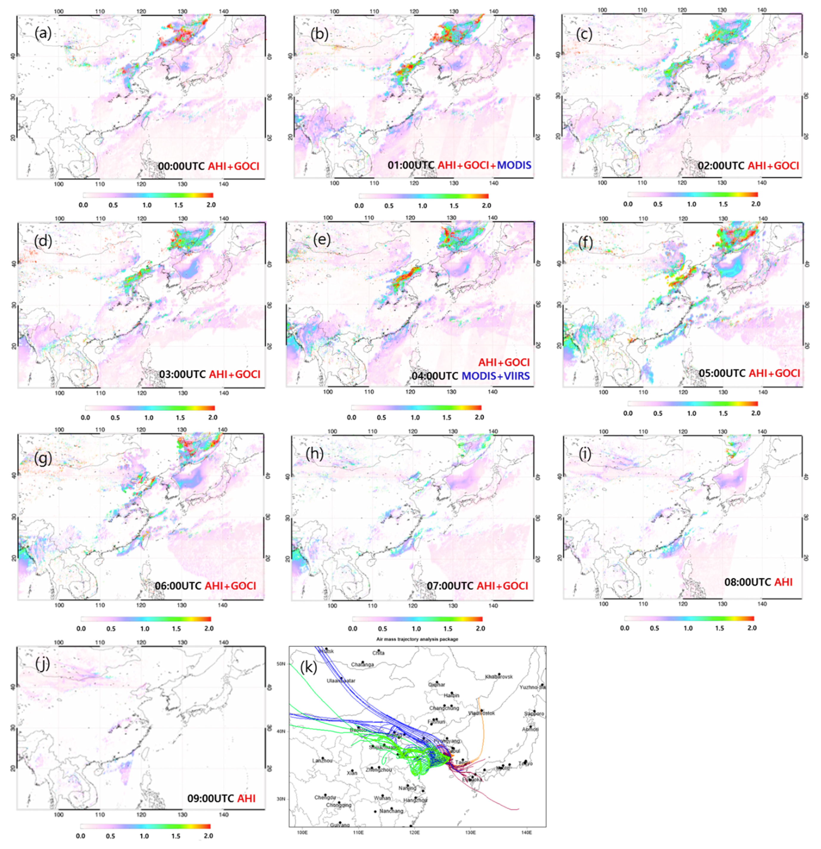
3.2.3. Case Studies: Composite Accuracy and Air Pollution Source Tracking
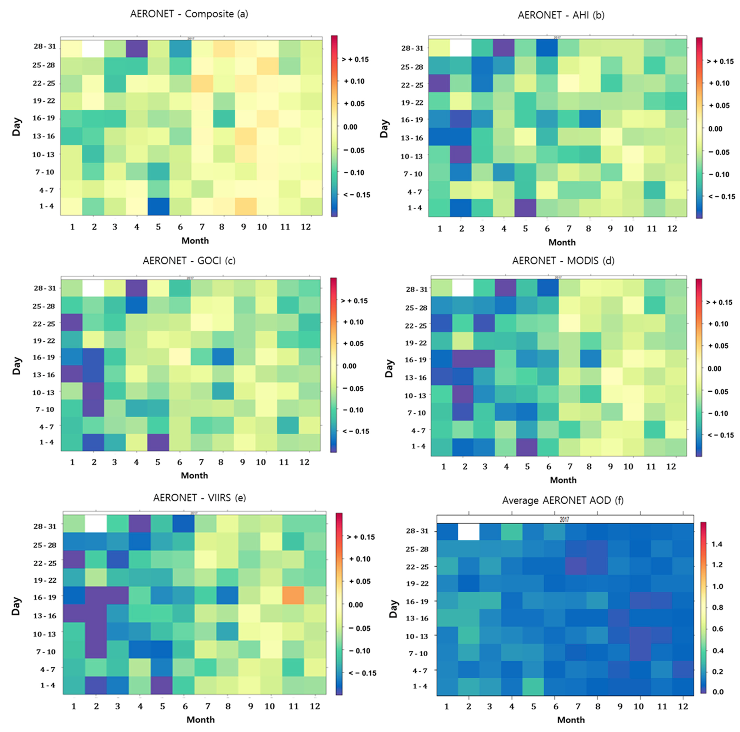
3.3. Long-Term Accuracy of AOD Composite
3.3.1. Evaluation of Composite and Satellite AOD
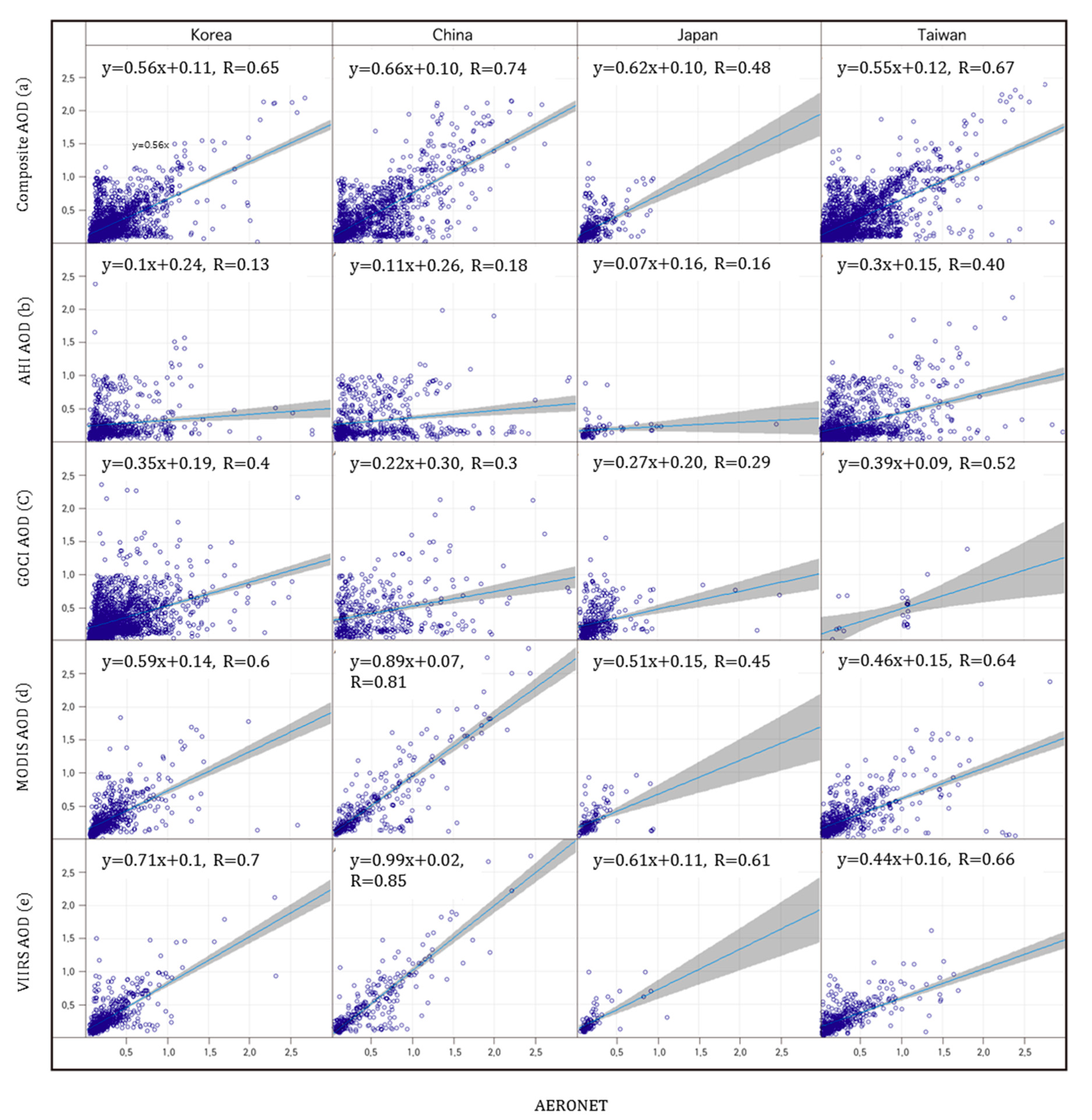
3.3.2. Regional Composite and Satellites Retrieval Accuracy
3.3.3. Composite AOD Accuracy Assessment
3.3.4. Limitations of Composite AOD
4. Summary and Conclusions
Author Contributions
Funding
Institutional Review Board Statement
Informed Consent Statement
Data Availability Statement
Acknowledgments
Conflicts of Interest
Abbreviations
| ADAM3 | Asian Dust Aerosol Model 3 |
| AOD | aerosol optical depth |
| CDF | cumulative distribution function |
| EDR | environmental data record |
| GEO | geosynchronous equatorial orbit |
| ICW | inverse composite weighting |
| IDW | inverse distance weighting |
| LEO | low earth orbit |
Appendix A

| AERONET Sites | Himawari-8 AHI | a0 | a1 | a2 | a3 |
|---|---|---|---|---|---|
| Anmyon | a0 + a1 X + a2 X2 + a3 X3 | 0.074 | −0.133 | 0.007 | 0.018 |
| Baengnyeong | a0 + a1 X + a2 X2 + a3 X3 | 0.026 | −0.072 | 0.029 | −0.119 |
| Beijing-CAMS | a0 + a1 X + a2 X2 + a3 X3 | 0.035 | −0.072 | 0.005 | 0.010 |
| Beijing | a0 + a1 X + a2 X2 + a3 X3 | 0.148 | −0.077 | 0.006 | 0.096 |
| Bhola | a0 + a1 X + a2 X2 + a3 X3 | 0.096 | −0.351 | 0.024 | 0.052 |
| Chen−Kung_Univ. | a0 + a1 X + a2 X2 + a3 X3 | 0.128 | 0.023 | −0.021 | 0.019 |
| Chiang_Mai_Met_Sta | a0 + a1 X + a2 X2 + a3 X3 | 0.287 | 0.144 | −0.043 | 0.015 |
| Dalanzadgad | a0 + a1 X + a2 X2 + a3 X3 | 0.205 | −0.051 | −0.017 | 0.018 |
| Dhaka−Univ. | a0 + a1 X + a2 X2 + a3 X3 | 0.331 | −0.697 | 0.087 | 0.013 |
| Dongsha_Island | a0 + a1 X + a2 X2 + a3 X3 | 0.001 | −0.116 | 0.022 | 0.051 |
| Doi_Ang−Khang | a0 + a1 X + a2 X2 + a3 X3 | 0.018 | −0.118 | −0.002 | 0.092 |
| EPA−NCU | a0 + a1 X + a2 X2 + a3 X3 | 0.002 | −0.251 | 0.024 | 0.058 |
| Fukuoka | a0 + a1 X + a2 X2 + a3 X3 | 0.061 | −0.413 | 0.054 | 0.068 |
| Gangneung_WNU | a0 + a1 X + a2 X2 + a3 X3 | 0.190 | −0.268 | 0.022 | 0.045 |
| Gosan_SNU | a0 + a1 X + a2 X2 + a3 X3 | 0.152 | −0.334 | 0.045 | −0.058 |
| Hongkong_PolyU | a0 + a1 X + a2 X2 + a3 X3 | 0.156 | −0.458 | 0.062 | −0.083 |
| Irkutsk | a0 + a1 X + a2 X2 + a3 X3 | 0.544 | −0.012 | −0.038 | 0.041 |
| NGHIA_DO | a0 + a1 X + a2 X2 + a3 X3 | 0.055 | −0.194 | 0.031 | −0.033 |
| Noto | a0 + a1 X + a2 X2 + a3 X3 | 0.043 | −0.208 | 0.120 | 0.063 |
| Omkoi | a0 + a1 X + a2 X2 + a3 X3 | 0.344 | −0.375 | 0.038 | 0.101 |
| Seoul_SNU | a0 + a1 X + a2 X2 + a3 X3 | 0.082 | −0.541 | 0.081 | 0.082 |
| Shirahama | a0 + a1 X + a2 X2 + a3 X3 | 0.044 | −0.194 | 0.007 | 0.027 |
| Son_La | a0 + a1 X + a2 X2 + a3 X3 | 0.091 | −0.593 | 0.102 | 0.084 |
| Taipei_CWB | a0 + a1 X + a2 X2 + a3 X3 | 0.023 | −0.232 | −0.004 | 0.019 |
| Ussuriysk | a0 + a1 X + a2 X2 + a3 X3 | 0.038 | −0.162 | −0.014 | 0.012 |
| XiangHe | a0 + a1 X + a2 X2 + a3 X3 | 0.004 | 0.061 | −0.014 | 0.012 |
| Yonsei_Univ. | a0 + a1 X + a2 X2 + a3 X3 | 0.096 | −0.308 | 0.034 | 0.057 |
| AERONET Sites | COMS GOCI | a0 | a1 | a2 | a3 |
|---|---|---|---|---|---|
| Anmyon | a0 + a1 X + a2 X2 + a3 X3 | 0.074 | 2.703 | 0.003 | 0.000 |
| Baengnyeong | a0 + a1 X + a2 X2 + a3 X3 | 0.143 | 0.044 | 0.013 | 0.109 |
| Beijing-CAMS | a0 + a1 X + a2 X2 + a3 X3 | 0.044 | 0.735 | 0.021 | 0.003 |
| Beijing | a0 + a1 X + a2 X2 + a3 X3 | 0.038 | 0.912 | −0.025 | 1.010 |
| Bhola | |||||
| Chen−Kung_Univ. | |||||
| Chiang_Mai_Met_Sta | |||||
| Dalanzadgad | |||||
| Dhaka−Univ. | |||||
| Dongsha_Island | |||||
| Doi_Ang−Khang | |||||
| EPA−NCU | a0 + a1 X + a2 X2 + a3 X3 | 0.012 | 1.296 | −0.187 | 0.001 |
| Fukuoka | a0 + a1 X + a2 X2 + a3 X3 | −0.143 | 1.438 | −0.147 | 0.001 |
| Gangneung_WNU | a0 + a1 X + a2 X2 + a3 X3 | 0.058 | 0.477 | 0.570 | 0.001 |
| Gosan_SNU | a0 + a1 X + a2 X2 + a3 X3 | 0.023 | 0.864 | 0.056 | 0.001 |
| Hongkong_PolyU | |||||
| Irkutsk | |||||
| NGHIA_DO | |||||
| Noto | a0 + a1 X + a2 X2 + a3 X3 | 0.175 | −0.191 | 0.021 | −0.021 |
| Omkoi | |||||
| Seoul_SNU | a0 + a1 X + a2 X2 + a3 X3 | −0.049 | 0.838 | −0.021 | 0.002 |
| Shirahama | a0 + a1 X + a2 X2 + a3 X3 | 0.023 | 1.324 | −0.431 | 0.001 |
| Son_La | |||||
| Taipei_CWB | a0 + a1 X + a2 X2 + a3 X3 | 0.059 | 1.388 | −0.290 | 0.001 |
| Ussuriysk | a0 + a1 X + a2 X2 + a3 X3 | 0.034 | 0.793 | −0.195 | 0.000 |
| XiangHe | a0 + a1 X + a2 X2 + a3 X3 | 0.036 | 0.998 | 0.135 | 0.684 |
| Yonsei_Univ. | a0 + a1 X + a2 X2 + a3 X3 | 0.034 | 0.900 | 0.059 | 1.051 |
| AERONET Sites | Terra, Aqua MODIS | a0 | a1 | a2 | a3 |
|---|---|---|---|---|---|
| Anmyon | a0 + a1 X + a2 X2 + a3 X3 | 0.074 | 2.703 | 0.003 | 0.000 |
| Baengnyeong | a0 + a1 X + a2 X2 + a3 X3 | 0.067 | −0.007 | −0.058 | 0.009 |
| Beijing-CAMS | a0 + a1 X + a2 X2 + a3 X3 | 2.211 | 0.081 | 0.007 | 0.006 |
| Beijing | a0 + a1 X + a2 X2 + a3 X3 | 2.360 | 1.924 | 0.008 | 0.003 |
| Bhola | a0 + a1 X + a2 X2 + a3 X3 | 1.900 | 4.394 | 0.003 | 0.001 |
| Chen−Kung_Univ. | a0 + a1 X + a2 X2 + a3 X3 | 2.056 | 2.996 | 0.004 | 0.002 |
| Chiang_Mai_Met_Sta | a0 + a1 X + a2 X2 + a3 X3 | −0.249 | 3.419 | 0.002 | 0.003 |
| Dalanzadgad | a0 + a1 X + a2 X2 + a3 X3 | −0.134 | 0.644 | 0.002 | 0.003 |
| Dhaka−Univ. | a0 + a1 X + a2 X2 + a3 X3 | 0.891 | 3.390 | 0.004 | 0.000 |
| Dongsha_Island | a0 + a1 X + a2 X2 + a3 X3 | −0.559 | 1.871 | 0.145 | 0.152 |
| Doi_Ang−Khang | a0 + a1 X + a2 X2 + a3 X3 | −1.041 | 3.621 | 0.005 | 0.003 |
| EPA−NCU | a0 + a1 X + a2 X2 + a3 X3 | −0.482 | 2.302 | 0.002 | 0.002 |
| Fukuoka | a0 + a1 X + a2 X2 + a3 X3 | −1.172 | 2.937 | 0.003 | 0.001 |
| Gangneung_WNU | a0 + a1 X + a2 X2 + a3 X3 | −1.225 | 2.614 | 0.004 | 0.002 |
| Gosan_SNU | a0 + a1 X + a2 X2 + a3 X3 | −1.166 | 3.366 | 0.003 | 0.001 |
| Hongkong_PolyU | a0 + a1 X + a2 X2 + a3 X3 | 0.453 | 2.793 | 0.003 | 0.000 |
| Irkutsk | a0 + a1 X + a2 X2 + a3 X3 | −0.354 | 1.462 | 0.001 | 0.002 |
| NGHIA_DO | a0 + a1 X + a2 X2 + a3 X3 | 0.096 | −0.389 | 0.001 | 0.150 |
| Noto | a0 + a1 X + a2 X2 + a3 X3 | 0.078 | −0.332 | 0.058 | 0.098 |
| Omkoi | a0 + a1 X + a2 X2 + a3 X3 | 0.295 | 2.091 | 0.002 | 0.000 |
| Seoul_SNU | a0 + a1 X + a2 X2 + a3 X3 | 2.824 | 2.907 | 0.004 | 0.002 |
| Shirahama | a0 + a1 X + a2 X2 + a3 X3 | 0.880 | 1.930 | 0.002 | 0.000 |
| Son_La | a0 + a1 X + a2 X2 + a3 X3 | −0.142 | 2.561 | 0.034 | 0.028 |
| Taipei_CWB | a0 + a1 X + a2 X2 + a3 X3 | 2.560 | 2.795 | −1.220 | 0.001 |
| Ussuriysk | a0 + a1 X + a2 X2 + a3 X3 | −4.129 | 4.903 | 0.081 | 0.012 |
| XiangHe | a0 + a1 X + a2 X2 + a3 X3 | 3.890 | 4.613 | 0.006 | 0.002 |
| Yonsei_Univ. | a0 + a1 X + a2 X2 + a3 X3 | 3.113 | 2.958 | 0.004 | 0.000 |
| AERONET Sites | Suomi-NPP VIIRS | a0 | a1 | a2 | a3 |
|---|---|---|---|---|---|
| Anmyon | a0 + a1 X + a2 X2 + a3 X3 | 3.012 | 2.703 | 0.003 | 0.000 |
| Baengnyeong | a0 + a1 X + a2 X2 + a3 X3 | 0.057 | −0.330 | 0.031 | 0.021 |
| Beijing-CAMS | a0 + a1 X + a2 X2 + a3 X3 | −1.873 | 0.988 | 2.162 | 1.010 |
| Beijing | a0 + a1 X + a2 X2 + a3 X3 | −1.870 | 0.576 | 1.801 | 0.003 |
| Bhola | a0 + a1 X + a2 X2 + a3 X3 | −1.880 | 0.271 | 2.783 | 0.002 |
| Chen−Kung_Univ. | a0 + a1 X + a2 X2 + a3 X3 | −3.284 | 0.571 | 0.187 | 1.446 |
| Chiang_Mai_Met_Sta | a0 + a1 X + a2 X2 + a3 X3 | 0.115 | 3.055 | 0.004 | 0.009 |
| Dalanzadgad | a0 + a1 X + a2 X2 + a3 X3 | 0.061 | 0.449 | 0.003 | 0.003 |
| Dhaka−Univ. | a0 + a1 X + a2 X2 + a3 X3 | −3.810 | 0.310 | 0.003 | 0.000 |
| Dongsha_Island | a0 + a1 X + a2 X2 + a3 X3 | −1.054 | 2.363 | 0.003 | 0.001 |
| Doi_Ang−Khang | a0 + a1 X + a2 X2 + a3 X3 | 2.306 | 0.886 | 0.004 | 0.001 |
| EPA−NCU | a0 + a1 X + a2 X2 + a3 X3 | −2.434 | 4.254 | 0.005 | 0.001 |
| Fukuoka | a0 + a1 X + a2 X2 + a3 X3 | −3.952 | 5.716 | 0.003 | 0.001 |
| Gangneung_WNU | a0 + a1 X + a2 X2 + a3 X3 | 1.447 | −1.642 | −0.532 | 0.001 |
| Gosan_SNU | a0 + a1 X + a2 X2 + a3 X3 | −1.665 | 3.865 | 0.004 | 0.001 |
| Hongkong_PolyU | a0 + a1 X + a2 X2 + a3 X3 | 0.487 | 1.854 | 0.000 | 0.010 |
| Irkutsk | a0 + a1 X + a2 X2 + a3 X3 | −0.419 | 1.527 | 0.004 | 0.002 |
| NGHIA_DO | a0 + a1 X + a2 X2 + a3 X3 | 0.075 | −0.577 | 0.093 | 0.112 |
| Noto | a0 + a1 X + a2 X2 + a3 X3 | 0.062 | −0.412 | 0.061 | 0.085 |
| Omkoi | a0 + a1 X + a2 X2 + a3 X3 | −0.328 | 2.214 | 0.003 | 0.005 |
| Seoul_SNU | a0 + a1 X + a2 X2 + a3 X3 | −0.729 | 3.079 | 0.004 | 0.002 |
| Shirahama | a0 + a1 X + a2 X2 + a3 X3 | −2.624 | 3.674 | 0.003 | 0.001 |
| Son_La | a0 + a1 X + a2 X2 + a3 X3 | 0.405 | 2.245 | 0.002 | 0.010 |
| Taipei_CWB | a0 + a1 X + a2 X2 + a3 X3 | −2.322 | 0.622 | 0.004 | 0.001 |
| Ussuriysk | a0 + a1 X + a2 X2 + a3 X3 | −0.097 | 0.883 | 0.372 | 0.001 |
| XiangHe | a0 + a1 X + a2 X2 + a3 X3 | −2.500 | −0.561 | 0.038 | 0.684 |
| Yonsei_Univ. | a0 + a1 X + a2 X2 + a3 X3 | −2.670 | 0.610 | 0.250 | 1.051 |
| Comparison | Season | N | R | RMSE | MB | MAE |
|---|---|---|---|---|---|---|
| Composite- AERONET | Spring | 1372 | 0.64 | 0.24 | −0.08 | 0.14 |
| Summer | 800 | 0.74 | 0.27 | −0.04 | 0.13 | |
| Fall | 1860 | 0.57 | 0.26 | 0.00 | 0.10 | |
| Winter | 2034 | 0.71 | 0.22 | −0.06 | 0.14 | |
| AHI-AE RONET | Spring | 748 | 0.22 | 0.37 | −0.10 | 0.17 |
| Summer | 320 | 0.48 | 0.34 | −0.08 | 0.11 | |
| Fall | 669 | 0.13 | 0.23 | −0.06 | 0.09 | |
| Winter | 778 | 0.17 | 0.36 | −0.11 | 0.16 | |
| GOCI-AERONET | Spring | 963 | 0.28 | 0.38 | −0.09 | 0.17 |
| Summer | 422 | 0.50 | 0.35 | −0.06 | 0.12 | |
| Fall | 786 | 0.39 | 0.24 | −0.06 | 0.09 | |
| Winter | 658 | 0.22 | 0.35 | −0.12 | 0.15 | |
| MODIS-AERONET | Spring | 184 | 0.60 | 0.17 | −0.14 | 0.16 |
| Summer | 238 | 0.46 | 0.15 | −0.08 | 0.11 | |
| Fall | 736 | 0.76 | 0.26 | −0.05 | 0.09 | |
| Winter | 648 | 0.75 | 0.25 | −0.12 | 0.15 | |
| VIIRS-AERONET | Spring | 150 | 0.73 | 0.16 | −0.14 | 0.15 |
| Summer | 193 | 0.83 | 0.15 | −0.08 | 0.11 | |
| Fall | 573 | 0.75 | 0.24 | −0.06 | 0.09 | |
| Winter | 467 | 0.70 | 0.14 | −0.13 | 0.15 |
| Comparison | Region | N | R | RMSE | MB | MAE |
|---|---|---|---|---|---|---|
| Composite-AERONET | Korea | 2064 | 0.65 | 0.23 | −0.08 | 0.14 |
| China | 1313 | 0.74 | 0.30 | −0.06 | 0.23 | |
| Japan | 353 | 0.48 | 0.18 | −0.01 | 0.06 | |
| Taiwan | 2336 | 0.67 | 0.21 | −0.03 | 0.12 | |
| AHI-AERONET | Korea | 680 | 0.13 | 0.34 | −0.12 | 0.15 |
| China | 557 | 0.18 | 0.35 | −0.17 | 0.22 | |
| Japan | 76 | 0.16 | 0.17 | −0.03 | 0.05 | |
| Taiwan | 1202 | 0.40 | 0.32 | −0.06 | 0.12 | |
| GOCI-AERONET | Korea | 2011 | 0.40 | 0.35 | −0.06 | 0.16 |
| China | 389 | 0.30 | 0.37 | −0.15 | 0.25 | |
| Japan | 401 | 0.29 | 0.20 | −0.01 | 0.08 | |
| Taiwan | 28 | 0.52 | 0.31 | −0.10 | 0.10 | |
| MODIS-AERONET | Korea | 675 | 0.60 | 0.14 | −0.12 | 0.15 |
| China | 356 | 0.81 | 0.29 | −0.16 | 0.23 | |
| Japan | 130 | 0.45 | 0.16 | −0.03 | 0.05 | |
| Taiwan | 645 | 0.64 | 0.21 | −0.08 | 0.11 | |
| VIIRS-AERONET | Korea | 575 | 0.70 | 0.14 | −0.13 | 0.14 |
| China | 288 | 0.85 | 0.37 | −0.17 | 0.22 | |
| Japan | 82 | 0.61 | 0.16 | −0.04 | 0.05 | |
| Taiwan | 438 | 0.66 | 0.11 | −0.09 | 0.11 |
References
- Kaufman, Y.J.; Didier, T.; Olivier, B. A satellite view of aerosols in the climate system. Nature 2002, 419, 215–223. [Google Scholar] [CrossRef] [PubMed]
- Adler, G.; Haspel, C.; Moise, T.; Rudich, Y. Optical extinction of highly porous aerosol following atmospheric freeze drying. J. Geophys. Res. Atmos. 2014, 119, 6768–6787. [Google Scholar] [CrossRef]
- Ghan, S.J.; Liu, X.; Easter, R.C.; Zaveri, R.; Rasch, P.J.; Yoon, J.-H.; Eaton, B. Toward a minimal representation of aerosols in climate models: Comparative decomposition of aerosol direct, semidirect, and indirect radiative forcing. J. Clim. 2012, 25, 6461–6476. [Google Scholar] [CrossRef]
- Zhang, K.; Wan, H.; Liu, X.; Ghan, S.J.; Kopperman, G.J.; Ma, P.-L.; Rasch, P.J. On the use of nudging for aerosol–climate model intercomparison studies. Atmos. Chem. Phys. 2014, 14, 8631–8645. [Google Scholar] [CrossRef] [Green Version]
- Tiwari, S.; Ramachandran, S. Study of aerosol-cloud interaction over Indo-Gangetic Basin during normal monsoon and drought years. In Proceedings of the American Geophysical Union, Fall Meeting, New Orleans, LA, USA, 11–15 December 2017. Abstract #A51G-2149. [Google Scholar]
- Haywood, J.; Boucher, O. Estimates of the direct and indirect radiative forcing due to tropospheric aerosols: A review. Rev. Geophys. 2000, 38, 513–543. [Google Scholar] [CrossRef]
- Heald, C.L.; Henze, D.K.; Horowitz, L.W.; Feddema, J.; Lamarque, J.-F.; Guenther, A.; Hess, P.G.; Vitt, F.; Seinfeld, J.H.; Goldstein, A.H.; et al. Predicted change in global secondary organic aerosol concentrations in response to future climate, emissions, and land use change. J. Geophys. Res. 2008, 113, D05211. [Google Scholar] [CrossRef]
- Anderson, T.L.; Charlson, R.J.; Schwartz, S.E.; Knutti, R.; Boucher, O.; Rodhe, H.; Heintzenberg, J. Climate forcing by Aerosols—A hazy picture. Science 2003, 300, 1103–1104. [Google Scholar] [CrossRef] [PubMed]
- Ramachandran, S.; Rengarajan, R.; Sarin, M.M. Atmospheric carbonaceous aerosols: Issues, radiative forcing and climate impacts. Curr. Sci. 2009, 97, 18–20. [Google Scholar]
- Engel-Cox, J.A.; Christopher, H.H.; Coutant, B.W.; Hoff, R.M. Qualitative and quantitative evaluation of MODIS satellite sensor data for regional and urban scale air quality. Atmos. Environ. 2004, 38, 2495–2509. [Google Scholar] [CrossRef]
- Dokery, D.W.; CAPope Xiping, X.; Spengler, J.; Ware, J.; Fay, M. An association between air pollution and mortality in 6 US cities. N. Engl. J. Med. 1993, 329, 1735–1739. [Google Scholar]
- Pope, C.A., III; Ezzati, M.; Dockery, D.W. Fine-particulate air pollution and life expectancy in the United States. N. Engl. J. Med. 2009, 360, 376–386. [Google Scholar] [CrossRef] [Green Version]
- Van Donkelaar, A.; Martin, R.V.; Brauer, M.; Kahn, R.; Levy, R.; Verduzco, C.; Villeneuve, P. Global estimates of ambient fine particulate matter concentrations from satellite-based aerosol optical depth: Development and application. Environ. Health Perspect. 2010, 118, 847–855. [Google Scholar] [CrossRef] [PubMed] [Green Version]
- Lim, S.; Lee, M.; Lee, G.; Kim, S.; Yoon, S.; Kang, K. Ionic and carbonaceous compositions of PM 10, PM 2.5 and PM 1.0 at Gosan ABC Superstation and their ratios as source signature. Atmos. Chem. Phys. 2012, 12, 2007–2024. [Google Scholar] [CrossRef] [Green Version]
- Chan, C.; Chan, L. Effect of meteorology and air pollutant transport on ozone episodes at a subtropical coastal Asian city, Hong Kong. J. Geophys. Res. Atmos. 2000, 105, 20707–20724. [Google Scholar] [CrossRef] [Green Version]
- Radojevic, M. Chemistry of forest fires and regional haze with emphasis on Southeast Asia. Pure Appl. Geophys. 2003, 160, 157–187. [Google Scholar] [CrossRef]
- Luan, Y.; Jaeglé, L. Composite study of aerosol export events from East Asia and North America. Atmos. Chem. Phys. 2013, 13, 1221–1242. [Google Scholar] [CrossRef] [Green Version]
- Zhang, W.; Gu, X.; Xu, H.; Yu, T.; Zheng, F. Assessment of OMI near-UV aerosol optical depth over Central and East Asia. J. Geophys. Res. Atmos. 2016, 121, 382–398. [Google Scholar] [CrossRef] [Green Version]
- Kaufman, Y.J.; Koren, I.; Remer, L.A.; Rosenfeld, D.; Rudich, Y. The effect of smoke, dust, and pollution aerosol on shallow cloud development over the Atlantic Ocean. Proc. Natl. Acad. Sci. USA 2005, 102, 11207–11212. [Google Scholar] [CrossRef] [Green Version]
- Kahn, R.A.; Gaitley, B.J.; Garay, M.J.; Diner, D.J.; Eck, T.F.; Smirnov, A.; Holben, B.N. Multiangle Imaging SpectroRadiometer global aerosol product assessment by comparison with the Aerosol Robotic Network. J. Geophys. Res. Atmos. 2010, 115. [Google Scholar] [CrossRef]
- Kinne, S. Remote sensing data combinations: Superior global maps for aerosol optical depth. In Satellite Aerosol Remote Sensing over Land; Kokhanovsky, A.A., de Leeuw, G., Eds.; Springer: Berlin, Germany, 2009. [Google Scholar]
- Shao, P.; Xin, J.; An, J.; Kong, L.; Wang, B.; Wang, J.; Wang, Y.; Wu, D. The empirical relationship between PM2.5 and AOD in Nanjing of the Yangtze River Delta. Atmos. Pollut. Res. 2017, 8, 233–243. [Google Scholar] [CrossRef]
- Zheng, Y.; Che, H.; Yang, L.; Chen, J.; Wang, Y.; Xia, X.; Zhao, H.; Wang, H.; Wang, D.; Gui, K. Optical and radiative properties of aerosols during a severe haze episode over the North China Plain in December. J. Meteorol. Res. 2016, 31, 1045–1061. [Google Scholar] [CrossRef]
- Dubovik, O.; Smirnov, A.; Holben, B.N.; King, M.D.; Kaufman, Y.J.; Eck, T.F.; Slutsker, I. Accuracy assessments of aerosol optical properties retrieved from Aerosol Robotic Network AERONET) Sun and sky radiance measurements. J. Geophys. Res. Atmos. 2000, 105, 9791–9806. [Google Scholar] [CrossRef] [Green Version]
- Creamean, J.; Suski, K.; Rosenfeld, D.; Cazorla, A.; DeMott, P.; Sullivan, R.; White, A.; Ralph, F.; Minnis, P.; Comstock, J.; et al. Dust and biological aerosols from the Sahara and Asia influence precipitation in the western US. Science 2013, 339, 1572–1578. [Google Scholar] [CrossRef] [PubMed] [Green Version]
- Van Donkelaar, A.; Martin, R.V.; Park, R.J. Estimating ground-level PM2.5 using aerosol optical depth determined from satellite remote sensing. J. Geophys. Res. Atmos. 2006, 111, D21. [Google Scholar] [CrossRef]
- Wang, J.; Christopher, S.A. Intercomparison between satellite derived aerosol optical thickness and PM2.5 mass: Implications for air quality studies. Geophys. Res. Lett. 2003, 30, 2095. [Google Scholar] [CrossRef]
- Zhang, J.; Reid, J. A decadal regional and global trend analysis of the aerosol optical depth using a data-assimilation grade over-water MODIS and Level 2 MISR aerosol products. Atmos. Chem. Phys. 2010, 10, 10949–10963. [Google Scholar] [CrossRef] [Green Version]
- Levy, R.C.; Munchak, L.A.; Mattoo, S.; Patadia, F.; Remer, L.A.; Holz, R.E. Towards a long-term global aerosol optical depth record: Applying a consistent aerosol retrieval algorithm to MODIS and VIIRS-observed reflectance. Atmos. Meas. Tech. 2015, 8, 4083–4110. [Google Scholar] [CrossRef] [Green Version]
- Sorek-Hamer, M.; Kloog, I.; Koutrakis, P.; Strawa, A.W.; Chatfield, R.; Cohen, A.; Ridgway, W.L.; Broday, D.M. Assessment of PM2.5 concentrations over bright surfaces using MODIS satellite observations. Remote Sens. Environ. 2015, 163, 180–185. [Google Scholar] [CrossRef]
- Wei, J.; Li, Z.; Suj, L.; Peng, Y.; Liu, L.; He, L.; Qin, W.; Cribb, M. MODIS Collection 6.1 3 km resolution aerosol optical depth product: Global evaluation and uncertainty analysis. Atmos. Environ. 2020, 240, 117768. [Google Scholar] [CrossRef]
- Li, C.; Li, J. Impact of aerosol vertical distribution on aerosol optical depth retrieval from passive satellite sensors. Remote Sens. 2020, 12, 1524. [Google Scholar] [CrossRef]
- Xue, Y.; Xu, H.; Mei, L.; Guang, J.; Guo, J.; Li, Y.; Hou, T.; Li, C.; Yang, L.; He, X. Merging aerosol optical depth data from multiple satellite missions to view agricultural biomass burning in Central and East China. Atmos. Chem. Phys. Discuss. 2012, 12, 10461–10492. [Google Scholar]
- Zhang, X.; Tang, Q. Combining satellite precipitation and long-term ground observations for hydrological monitoring in China. J. Geophys. Res. Atmos. 2015, 120, 6426–6443. [Google Scholar] [CrossRef] [Green Version]
- Kokhanovsky, A.A.; Breon, F.M.; Cacciari, A.; Carboni, E.; Diner, D.; Di Nicolantonio, W.; Grainger, R.G.; Grey, W.M.F.; Holler, R.; Lee, K.-H.; et al. Aerosol remote sensing over land: A comparison of satellite retrievals using different algorithms and instruments. Atmos. Res. 2007, 85, 372–394. [Google Scholar] [CrossRef]
- De Leeuw, G.; Holzer-Popp, T.; Bevan, S.; Davies, W.; Descloitres, J.; Grainger, R.G.; Griesfeller, J.; Heckel, A.; Kinne, S.; Klüser, L. Evaluation of seven European aerosol optical depth retrieval algorithms for climate analysis. Remote Sens. Environ. 2015, 162, 295–315. [Google Scholar] [CrossRef] [Green Version]
- Nirala, M. Multi-sensor data fusion of aerosol optical thickness. Int. J. Remote Sens. 2008, 29, 2127–2136. [Google Scholar] [CrossRef]
- Heo, J.-H.; Ryu, G.-H.; Sohn, E.-H.; Jang, J.-D. Application of Cumulative Distribution Functions to Compositing Precipitable Water with Low Earth Orbit Satellite Data. Asia-Pac. J. Atmos. Sci. 2020, 56, 57–75. [Google Scholar] [CrossRef]
- Wei, X.; Chang, N.B.; Bai, K.; Gao, W. Satellite remote sensing of aerosol optical depth: Advances, challenges, and perspectives. Crit. Rev. Environ. Sci. Technol. 2020, 50, 1640–1725. [Google Scholar] [CrossRef]
- Li, J.; Li, X.; Carlson, B.E.; Kahn, R.A.; Lacis, A.A.; Dubovik, O.; Nakajima, T. Reducing multisensor satellite monthly mean aerosol optical depth uncertainty: 1. Objective assessment of current AERONET locations. J. Geophys. Res. Atmos. 2016, 121, 13,609–13,627. [Google Scholar] [CrossRef] [PubMed]
- Kidder, S.Q.; Jones, A.S. A blended satellite total precipitable water product for operational forecasting. J. Atmos. Ocean. Technol. 2007, 24, 74–81. [Google Scholar] [CrossRef] [Green Version]
- Heo, J.H.; Ryu, G.-H.; Jang, J.-D. Optimal interpolation of precipitable water using low earth orbit and numerical weather prediction data. Remote Sens. 2018, 10, 436. [Google Scholar]
- Bain, L.J. Statistical Analysis of Reliability and Life Testing Model; Marceland Dekker Inc.: New York, NY, USA, 1976. [Google Scholar]
- Yumimoto, K.; Nagao, T.M.; Kikuchi, M.; Sekiyama, T.T.; Murakami, H.; Tanaka, T.Y.; Ogi, A.; Irie, H.; Khatri, P.; Okumura, H. Aerosol data assimilation using data from Himawari-8, a next-generation geostationary meteorological satellite. Geophys. Res. Lett. 2016, 43, 5886–5894. [Google Scholar] [CrossRef]
- Bessho, K.; Date, K.; Hayashi, M.; Ikeda, A.; Imai, T.; Inoue, H.; Kumagai, Y.; Miyakawa, T.; Murata, H.; Ohno, T.; et al. An introduction to Himawari-8/9—Japan’s new-generation geostationary meteorological satellites. J. Meteorol. Soc. Jpn. Ser. II 2016, 94, 151–183. [Google Scholar] [CrossRef] [Green Version]
- Yan, X.; Li, Z.; Luo, N.; Shi, W.; Zhao, W.; Yang, X.; Jin, J. A minimum albedo aerosol retrieval method for the new-generation geostationary meteorological satellite Himawari-8. Atmos. Res. 2018, 207, 14–27. [Google Scholar] [CrossRef]
- Yumimoto, K.; Tanaka, T.Y.; Yoshida, M.; Kikuchi, M.; Nagao, T.M.; Murakami, H.; Maki, T. Assimilation and forecasting experiment for heavy Siberian wildfire smoke in May 2016 with Himawari-8 aerosol optical thickness. J. Meteorol. Soc. Jpn. Ser. II 2018. [Google Scholar] [CrossRef] [Green Version]
- Fukuda, S.; Nakajima, T.; Takenaka, H.; Higurashi, A.; Kikuchi, N.; Nakajima, T.Y.; Ishida, H. New approaches to removing cloud shadows and evaluating the 380 nm surface reflectance for improved aerosol optical thickness retrievals from the GOSAT/TANSO-Cloud and Aerosol Imager. J. Geophys. Res. Atmos. 2013, 118, 13,520–13,531. [Google Scholar] [CrossRef]
- Yoshida, M.; Kikuchi, M.; Nagao, T.M.; Murakami, H.; Nomaki, T.; Higurash, A. Common retrieval of aerosol properties for imaging satellite sensors. J. Meteorol. Soc. Jpn. Ser. II 2018. [Google Scholar] [CrossRef] [Green Version]
- Wang, W.; Mao, F.; Pan, Z.; Gong, W.; Yoshida, M.; Zou, B.; Ma, H. Evaluating aerosol optical depth from Himawari-8 with Sun photometer network. J. Geophys. Res. Atmos. 2019, 124, 5516–5538. [Google Scholar] [CrossRef]
- Choi, J.K.; Park, Y.J.; Ahn, J.H.; Lim, H.S.; Eom, J.; Ryu, J.H. GOCI, the world’s first geostationary ocean color observation satellite, for the monitoring of temporal variability in coastal water turbidity. J. Geophys. Res. Ocean. 2012, 117. [Google Scholar] [CrossRef]
- Choi, M.; Kim, J.; Lee, J.; Kim, M.; Je Park, Y.; Jeong, U.; Kim, W.; Holben, B.; Eck, T.F.; Lim, J.H.; et al. GOCI Yonsei Aerosol Retrieval (YAER) algorithm and validation during DRAGON-NE Asia 2012 campaign. Atmos. Meas. Tech. Discuss. 2015, 8, 9565–9609. [Google Scholar]
- Choi, M.; Kim, J.; Lee, J.; Kim, M.; Park, Y.-J.; Holben, B.; Eck, T.F.; Li, Z.; Song, C.H. GOCI Yonsei aerosol retrieval version 2 products: An improved algorithm and error analysis with uncertainty estimation from 5-year validation over East Asia. Atmos. Meas. Tech. 2018, 11, 385–408. [Google Scholar] [CrossRef] [Green Version]
- Kaufman, Y.J.; Tanre, D. Strategy for direct and indirect methods for correcting the aerosol effect on remote sensing: From AVHRR to EOS-MODIS. Remote Sens. Environ. 1996, 55, 65–79. [Google Scholar] [CrossRef]
- Levy, R.C.; Remer, L.A.; Kleidman, R.G.; Mattoo, S.; Ichoku, C.; Kahn, R.; Eck, T.F. Global evaluation of the Collection 5 MODIS dark-target aerosol products over land. Atmos. Chem. Phys. 2010, 10, 10399–10420. [Google Scholar] [CrossRef] [Green Version]
- Bilal, M.; Nichol, J.E. Evaluation of MODIS aerosol retrieval algorithms over the Beijing-Tianjin-Hebei region during low to very high pollution events. J. Geophys. Res. Atmos. 2015, 120, 7941–7957. [Google Scholar] [CrossRef] [Green Version]
- Levy, R.C.; Mattoo, S.; Munchak, L.A.; Remer, L.A.; Sayer, A.M.; Patadia, F.; Hsu, N.C. The Collection 6 MODIS aerosol products over land and ocean. Atmos. Meas. Tech. 2013, 6, 2989. [Google Scholar] [CrossRef] [Green Version]
- Nichol, J.; Bilal, M. Validation of MODIS 3 km resolution aerosol optical depth retrievals over Asia. Remote Sens. 2016, 8, 328. [Google Scholar] [CrossRef] [Green Version]
- Remer, L.A.; Kaufman, Y.J.; Tanré, D.; Mattoo, S.; Chu, D.A.; Martins, J.V.; Li, R.R.; Ichoku, C.; Levy, R.C.; Kleidman, R.G.; et al. The MODIS aerosol algorithm, products, and validation. J. Atmos. Sci. 2005, 62, 947–973. [Google Scholar] [CrossRef] [Green Version]
- Chu, D.; Ichoku, C.; Remer, L.A.; Tanre, D.; Holben, B.N. Validation of MODIS aerosol optical depth retrieval over land. Geophys. Res. Lett. 2002, 29, MOD2-1–MOD2-4. [Google Scholar] [CrossRef] [Green Version]
- Sayer, A.M.; Hsu, N.C.; Bettenhausen, C.; Jeong, M.-J. Validation and uncertainty estimates for MODIS Collection 6 Deep Blue aerosol data. J. Geophys. Res. Atmos. 2013, 118, 7864–7872. [Google Scholar] [CrossRef] [Green Version]
- Remer, L.A.; Mattoo, S.; Levy, R.C.; Munchak, L.A. MODIS 3 km aerosol product: Algorithm and global perspective. Atmos. Meas. Tech. 2013, 6, 1829–1844. [Google Scholar] [CrossRef] [Green Version]
- Huang, J.; Kondragunta, S.; Laszlo, I.; Liu, H.; Remer, L.A.; Zhang, H.; Superczynski, S.; Ciren, P.; Holben, B.N.; Petrenko, M. Validation and expected error estimation of Suomi-NPP VIIRS aerosol optical thickness and Ångström exponent with AERONET. J. Geophys. Res. Atmos. 2016, 121, 7139–7160. [Google Scholar] [CrossRef] [Green Version]
- Jackson, J.M.; Liu, H.; Laszlo, I.; Kondragunta, S.; Remer, L.A.; Huang, J.; Huang, H.C. Suomi-NPP VIIRS aerosol algorithms and data products. J. Geophys. Res. Atmos. 2013, 118, 12673–12689. [Google Scholar] [CrossRef]
- Kotchenova, S.Y.; Vermote, E.F. Validation of a vector version of the 6S radiative transfer code for atmospheric correction of satellite data. Part II. Homogeneous Lambertian and anisotropic surfaces. Appl. Opt. 2007, 46, 4455–4464. [Google Scholar] [CrossRef] [Green Version]
- Vermote, E.F.; Kotchenova, S. Atmospheric correction for the monitoring of land surfaces. J. Geophys. Res. Atmos. 2008, 113. [Google Scholar] [CrossRef]
- Holben, B.N.; Eck, T.F.; Slutsker, I.; Tanre, D.; Buis, J.P.; Setzer, A.; Vermote, E.; Reagan, J.A.; Kaufman, Y.J.; Nakajima, T.; et al. AERONET—A federated instrument network and data archive for aerosol characterization. Remote Sens. Environ. 1998, 66, 1–16. [Google Scholar] [CrossRef]
- Holben, B.N.; Tanre, D.; Smirnov, A.; Eck, T.F.; Slutsker, I.; Abuhassan, N.; Newcomb, W.W.; Schafer, J.; Chatenet, B.; Lavenue, F.; et al. An emerging ground-based aerosol climatology: Aerosol optical depth from AERONET. J. Geophys. Res. Atmos. 2001, 106, 12067–12097. [Google Scholar] [CrossRef]
- Shin, S.-K.; Tesche, M.; Müller, D.; Noh, Y. Absorption aerosol optical depth components from AERONET observations of mixed dust plumes. Atmos. Meas. Tech. 2019, 12, 607–618. [Google Scholar] [CrossRef] [Green Version]
- Dey, S.; Tripathi, S.N.; Singh, R.P.; Holben, B.N. Retrieval of black carbon and specific absorption over Kanpur city, northern India during 2001–2003 using AERONET data. Atmos. Environ. 2006, 40, 445–456. [Google Scholar] [CrossRef]
- Alam, K.; Trautmann, T.; Blaschke, T. Aerosol optical properties and radiative forcing over mega-city Karachi. Atmos. Res. 2011, 101, 773–782. [Google Scholar] [CrossRef]
- Alam, K.; Trautmann, T.; Blaschke, T.; Subhan, F. Changes in aerosol optical properties due to dust storms in the Middle East and Southwest Asia. Remote Sens. Environ. 2014, 143, 216–227. [Google Scholar] [CrossRef]
- Bibi, H.; Alam, K.; Chishtie, F. Intercomparison of MODIS, MISR, OMI, and CALIPSO aerosol optical depth retrievals for four locations on the Indo-Gangetic plains and validation against AERONET data. Atmos. Environ. 2015, 111, 113–126. [Google Scholar] [CrossRef]
- Holben, B.N.; Tanré, A.D.; Smirnov, T.F.; Eck, I.; Slutsker, O.; Dubovik, F.; Lavenu, N.; Abuhassen, C.B. Optical properties of aerosols from long term ground-based aeronet measurements. In Proceedings of the ALPS99, Meribel, France, 17–23 January 1999. [Google Scholar]
- Schmid, B.; Michalsky, J.; Ttalthore, R.; Beauharnois, M.; Harrison, L.; Livingston, J.; Russell, P.; Holben, B.; Eck, T.; Stairnov, A. Comparison of aerosol optical depth from four solar radiometers during the fall 1997 ARM intensive observation period. Geophys. Res. Lett. 1999, 26, 2725–2728. [Google Scholar] [CrossRef]
- Gupta, P.; Remer, L.A.; Levy, R.C.; Mattoo, S. Validation of MODIS 3 km land aerosol optical depth from NASA’s EOS Terra and Aqua missions. Atmos. Meas. Tech. 2018, 11, 3145–3159. [Google Scholar] [CrossRef] [Green Version]
- Deng, P.; Zhang, M.; Guo, H.; Xu, C.; Bing, J.; Jia, J. Error analysis and correction of the daily GSMaP products over Hanjiang River Basin of China. Atmos. Res. 2018, 214, 121–134. [Google Scholar] [CrossRef]
- Sheffield, J.; Wood, E.F.; Chaney, N.; Guan, K.; Sadri, S.; Yuan, X.; Demuth, S. A drought monitoring and forecasting system for sub-Sahara African water resources and food security. Bull. Am. Meteorol. Soc. 2014, 95, 861–882. [Google Scholar] [CrossRef]
- Liu, M.; Shen, Y.; Qi, Y.; Wang, Y.; Geng, X. Changes in precipitation and drought extremes over the past half century in China. Atmosphere 2019, 10, 203. [Google Scholar] [CrossRef] [Green Version]
- Reichle, R.H.; Koster, R.D. Bias reduction in short records of satellite soil moisture. Geophys. Res. Lett. 2004, 31, L19501. [Google Scholar] [CrossRef] [Green Version]
- Liu, Y.; van Dijk, A.I.J.M.; de Jeu, R.A.M.; Holmes, T.R.H. An analysis of spatiotemporal variations of soil and vegetation moisture from a 29-year satellite-derived data set over mainland Australia. Water Resour. Res. 2009, 45. [Google Scholar] [CrossRef] [Green Version]
- Klippel, S.; Wieczorek, M.; Schumann, M.; Krause, E.; Marg, B.; Seidel, T.; Meyer, T.; Knapp, E.W.; Freund, C. Multivalent binding of formin-binding protein 21 FBP21)-tandem-WW domains fosters protein recognition in the pre-spliceosome. J. Biol. Chem. 2011, 286, 38478–38487. [Google Scholar] [CrossRef] [PubMed] [Green Version]
- Nalder, I.A.; Wein, R.W. Spatial interpolation of climatic normals: Test of a new method in the Canadian boreal forest. Agric. For. Meteorol. 1998, 92, 211–225. [Google Scholar] [CrossRef]
- Chao, L.; Zhang, K.; Li, Z.; Zhu, Y.; Wang, J.; Yu, Z. Geographically weighted regression based methods for merging satellite and gauge precipitation. J. Hydrol. 2018, 558, 275–289. [Google Scholar] [CrossRef]
- Dinku, T.; Hailemariam, K.; Maidment, R.; Tarnavsky, E.; Connor, S. Combined use of satellite estimates and rain gauge observations to generate high-quality historical rainfall time series over Ethiopia. Int. J. Climatol. 2014, 34, 2489–2504. [Google Scholar] [CrossRef] [Green Version]
- Manz, B.; Buytaert, W.; Zulkafli, Z.; Lavado, W.; Willems, B.; Alberto Robles, L.; Rodriguez-Sanchez, J.-P. High-resolution satellite-gauge merged precipitation climatologies of the Tropical Andes. J. Geophys. Res. Atmos. 2016, 121, 1190–1207. [Google Scholar] [CrossRef] [Green Version]
- Lloyd, C. Assessing the effect of integrating elevation data into the estimation of monthly precipitation in Great Britain. J. Hydrol. 2005, 308, 128–150. [Google Scholar] [CrossRef]
- Draxler, R.R.; Hess, G. An overview of the HYSPLIT_4 modelling system for trajectories. Aust. Meteorol. Mag. 1998, 47, 295–308. [Google Scholar]
- Draxler, R.R. The use of global and mesoscale meteorological model data to predict the transport and dispersion of tracer plumes over Washington, DC. Weather Forecast. 2006, 21, 383–394. [Google Scholar] [CrossRef]
- Fleming, Z.L.; Monks, P.S.; Manning, A.J. Untangling the influence of air-mass history in interpreting observed atmospheric composition. Atmos. Res. 2012, 104, 1–39. [Google Scholar] [CrossRef] [Green Version]
- Efstathiou, C.; Isukapalli, S.; Georgopoulos, P. A mechanistic modeling system for estimating large-scale emissions and transport of pollen and co-allergens. Atmos. Environ. 2011, 45, 2260–2276. [Google Scholar] [CrossRef] [Green Version]
- Stunder, B.J.B.; Heffter, J.L.; Draxler, R.R. Airborne volcanic ash forecast area reliability. Weather Forecast. 2007, 22, 1132–1139. [Google Scholar] [CrossRef]
- Pasken, R.; Pietrowicz, J.A. Using dispersion and mesoscale meteorological models to forecast pollen concentrations. Atmos. Environ. 2005, 39, 7689–7701. [Google Scholar] [CrossRef]
- Chen, B.; Stein, A.F.; Maldonado, P.G.; de la Campa, A.M.S.; Gonzalez-Castanedo, Y.; Castell, N.; Jesus, D. Size distribution and concentrations of heavy metals in atmospheric aerosols originating from industrial emissions as predicted by the HYSPLIT model. Atmos. Environ. 2013, 71, 234–244. [Google Scholar] [CrossRef]
- Gaiero, D.M.; Simonella, L.; Gasso, S.; Gili, S.; Stein, A.F.; Soas, P. Ground/satellite observations and atmospheric modeling of dust storms originating in the high Puna-Altiplano deserts South America): Implications for the interpretation of paleo-climatic archives. J. Geophys. Res. Atmos. 2013, 118, 3817–3831. [Google Scholar] [CrossRef] [Green Version]
- Stein, A.F.; Isakov, V.; Godowitch, J.; Draxler, R.R. A hybrid modeling approach to resolve pollutant concentrations in an urban area. Atmos. Environ. 2007, 41, 9410–9426. [Google Scholar] [CrossRef]
- Bowyer, T.W.; Kephart, R.; Eslinger, P.W.; Friese, J.I.; Miley, H.S.; Saey, P.R.J. Maximum reasonable radioxenon releases from medical isotope production facilities and their effect on monitoring nuclear explosions. J. Environ. Radioact. 2013, 115, 192–200. [Google Scholar] [CrossRef]
- Jeong, H.; Park, M.; Jeong, H.; Hwang, W.; Kim, E.; Han, M. Radiological risk assessment caused by RDD terrorism in an urban area. Appl. Radiat. Isot. 2013, 79, 1–4. [Google Scholar] [CrossRef] [PubMed]
- Jiang, T.; Chen, B.; Chan, K.K.Y.; Xu, B. Himawari-8/AHI and MODIS aerosol optical depths in China: Evaluation and comparison. Remote Sens. 2019, 11, 1011. [Google Scholar] [CrossRef] [Green Version]
- Xiao, Q.; Zhang, H.; Choi, M.; Li, S.; Kondragunta, S.; Kim, J.; Holben, B.; Levy, R.C.; Liu, Y. Evaluation of VIIRS, GOCI, and MODIS Collection 6 AOD retrievals against ground sunphotometer observations over East Asia. Atmos. Chem. Phys. 2016, 16, 1255. [Google Scholar] [CrossRef] [Green Version]
- Bilal, M.; Nazeer, M.; Nichol, J.; Qiu, Z.; Wang, L.; Bleiweiss, M.P.; Lolli, S. Evaluation of Terra-MODIS C6 and C6. 1 aerosol products against Beijing, XiangHe, and Xinglong AERONET sites in China during 2004–2014. Remote Sens. 2019, 11, 486. [Google Scholar] [CrossRef] [Green Version]
- Qi, Y.; Ge, J.; Huang, J. Spatial and temporal distribution of MODIS and MISR aerosol optical depth over northern China and comparison with AERONET. Chin. Sci. Bull. 2013, 58, 2497–2506. [Google Scholar] [CrossRef] [Green Version]
- Wang, L.; Wang, J.X.; Li, Z.; Liu, G.; Li, J. Evaluation of the MODIS aerosol optical depth retrieval over different ecosystems in China during EAST-AIRE. Atmos. Environ. 2007, 41, 7138–7149. [Google Scholar] [CrossRef]
- Li, X.H.; Wang, S.X.; Duan, L.; Hao, J.M.; Nie, Y.F. Carbonaceous aerosol emissions from household biofuel combustion in China. Environ. Sci. Technol. 2009, 43, 6076–6081. [Google Scholar] [CrossRef] [PubMed]
- Anderson, J.C.; Wang, J.; Zeng, J.; Leptoukh, G.; Petrenko, M.; Ichoku, C.; Hu, C. Long-term statistical assessment of Aqua-MODIS aerosol optical depth over coastal regions: Bias characteristics and uncertainty sources. Tellus B Chem. Phys. Meteorol. 2013, 65, 20805. [Google Scholar] [CrossRef]
- Mhawish, A.; Banerjee, T.; Broday, D.M.; Misra, A. Evaluation of MODIS Collection 6 aerosol retrieval algorithms over Indo-Gangetic Plain: Implications of aerosols types and mass loading. Remote Sens. Environ. 2017, 201, 297–313. [Google Scholar] [CrossRef]
- He, L.J.; Wang, L.C.; Lin, A.W.; Zhang, M.; Bilal, M.; Wei, J. Performance of the NPP-VIIRS and Aqua-MODIS aerosol optical depth products over the Yangtze River Basin. Remote Sens. 2018, 10, 117. [Google Scholar] [CrossRef] [Green Version]
- Zhang, Z.; Wu, W.; Fan, M.; Wei, J.; Jin, J.; Tan, Y.; Wang, Q. Validation of Himawari-8 aerosol optical depth retrievals over China. Atmos. Environ. 2019, 199, 32–44. [Google Scholar] [CrossRef]
- Tao, J.; Zhang, L.; Cao, J.; Zhang, R. A review of current knowledge concerning PM 2.5 chemical composition, aerosol optical properties and their relationships across China. Atmos. Chem. Phys. 2017, 17, 9485. [Google Scholar] [CrossRef] [Green Version]
- Husar, R.; Tratt, D.M.; Schichtel, B.A. Asian dust events of April 1998. J. Geophys. Res. Atmos. 2001, 106, 18317–18330. [Google Scholar] [CrossRef]
- Wang, F.; Chen, D.S.; Cheng, S.Y.; Li, J.B.; Li, M.J.; Ren, Z.H. Identification of regional atmospheric PM10 transport pathways using HYSPLIT, MM5-CMAQ and synoptic pressure pattern analysis. Environ. Model. Softw. 2010, 25, 927–934. [Google Scholar] [CrossRef]
- He, L.; Wang, L.; Lin, A.; Zhang, M.; Bilal, M.; Tao, M. Aerosol optical properties and associated direct radiative forcing over the Yangtze River basin during 2001–2015. Remote Sens. 2017, 9, 746. [Google Scholar] [CrossRef] [Green Version]
- Cheng, Z.; Wang, S.X.; Jiang, J.K.; Fu, Q.Y.; Chen, C.H.; Xu, B.Y. Long-term trend of haze pollution and impact of particulate matter in the Yangtze River Delta, China. Environ. Pollut. 2013, 182, 101–110. [Google Scholar] [CrossRef]
- Li, B.; Zhang, J.; Zhao, Y.; Yuan, S.; Zhao, Q.; Shen, G.; Wu, H. Seasonal variation of urban carbonaceous aerosols in a typical city Nanjing in Yangtze River Delta, China. Atmos. Environ. 2015, 106, 223–231. [Google Scholar] [CrossRef]
- Knapp, K.R.; Vonder Haar, T.H.; Kaufman, Y.J. Aerosol optical depth retrieval from GOES-8: Uncertainty study and retrieval validation over South America. J. Geophys. Res. Atmos. 2002, 107, AAC 2-1–AAC 2-12. [Google Scholar] [CrossRef] [Green Version]
- Zhang, W.; Xu, H.; Zhang, L. Assessment of Himawari-8 AHI Aerosol Optical Depth Over Land. Remote Sens. 2019, 11, 1108. [Google Scholar] [CrossRef] [Green Version]
- Naeger, A.R.; Gupta, P.; Zavodsky, B.T.; McGrath, K.M. Monitoring and tracking the trans-Pacific transport of aerosols using multi-satellite aerosol optical depth composites. Atmos. Meas. Tech. 2016, 9, 2463–2482. [Google Scholar] [CrossRef] [Green Version]


| Satellite | Instrument/Orbit | Scientific Dataset Name | Resolution | Repeat Coverage |
|---|---|---|---|---|
| Himawari-8 | AHI/GEO | Hourly aerosol product at 500 nm | 00:00–09:00 UTC, 5 km | 10 min |
| COMS | GOCI/GEO | GOCI Yonsei Aerosol V2 product at 500 nm | 00:00–07:00 UTC, 0.5 km | 1 h |
| Aqua·Terra | MODIS/LEO | Deep_Blue_Aerosol_Optical_Depth_550_Land_Best_Estimate | 01:30/04:30 UTC, 10 km | 2× day−1 |
| Suomi-NPP | VIIRS/LEO | VIIRS_Aeros_EDR_GEO_ALL | 04:30 UTC, 6 km | 1× day−1 |
| AERONET Sites | Longitude (Degree) | Latitude (Degree) | Elevation (m) |
|---|---|---|---|
| Anmyon | 126.330 | 36.539 | 47 |
| Baengnyeong | 124.630 | 37.966 | 136 |
| Beijing-CAMS | 116.317 | 39.933 | 106 |
| Beijing | 116.381 | 39.754 | 36 |
| Bhola | 90.750 | 22.167 | 3 |
| Chen-Kung_Univ. | 120.217 | 23.000 | 50 |
| Chiang_Mai_Met_Sta | 98.972 | 18.771 | 312 |
| Dalanzadgad | 104.419 | 43.577 | 1470 |
| Dhaka_Univ. | 90.398 | 23.728 | 34 |
| Dongsha-Island | 116.729 | 20.699 | 5 |
| Doi-Ang-Khang | 99.045 | 19.932 | 1536 |
| EPA-NCU | 121.185 | 24.968 | 144 |
| Fukuoka | 130.475 | 33.524 | 30 |
| Gangneung-WNU | 128.867 | 37.771 | 60 |
| Gosan_SNU | 126.162 | 33.292 | 72 |
| Hongkong_PolyU | 114.117 | 22.483 | 40 |
| Irkutsk | 103.087 | 51.800 | 670 |
| NGHIA_DO | 105.800 | 21.048 | 40 |
| Noto | 137.137 | 37.334 | 200 |
| Omkoi | 98.432 | 17.798 | 1120 |
| Seoul_SNU | 126.951 | 37.458 | 116 |
| Shirahama | 135.357 | 33.693 | 10 |
| Son_La | 103.905 | 21.332 | 683 |
| Taipei_CWB | 121.500 | 25.030 | 26 |
| Ussuriysk | 132.163 | 43.700 | 280 |
| XiangHe | 116.962 | 39.754 | 36 |
| Yonsei_Uni. | 126.935 | 37.564 | 88 |
| AERONET Sites | AHI | GOCI | MODIS | VIIRS |
|---|---|---|---|---|
| Anmyon | 0.22/0.17 | 0.15/0.09 | 0.13/0.09 | 0.11/0.10 |
| Baengnyeong | 0.21/0.16 | 0.11/0.09 | 0.12/0.11 | 0.12/0.11 |
| Beijing-CAMS | 0.32/0.28 | 0.28/0.27 | 0.19/0.18 | 0.18/0.18 |
| Beijing | 0.32/0.28 | 0.28/0.27 | 0.19/0.18 | 0.18/0.18 |
| Bhola | 0.23/0.21 | - | 0.18/0.15 | 0.17/0.15 |
| Chen-Kung_Uni. | 0.16/0.09 | 0.21/0.09 | 0.09/0.08 | 0.09/0.08 |
| Chiang_Mai_Met_Sta | 0.24/0.18 | - | 0.16/0.14 | 0.14/0.13 |
| Dalanzadgad | 0.22/0.09 | - | 0.07/0.07 | 0.08/0.07 |
| Dhaka_Uni. | 0.32/0.28 | - | 0.13/0.11 | 0.13/0.12 |
| Dongsha-island | 0.14/0.12 | - | 0.08/0.08 | 0.07/0.07 |
| Doi-Ang-Khang | 0.16/0.15 | - | 0.19/0.15 | 0.17/0.14 |
| EPA-NCU | 0.28/0.18 | 0.22/0.08 | 0.09/0.09 | 0.09/0.09 |
| Fukuoka | 0.09/0.08 | 0.09/0.07 | 0.08/0.08 | 0.08/0.08 |
| Gangneung-WNU | 0.12/0.11 | 0.16/0.14 | 0.13/0.11 | 0.12/0.10 |
| Gosan_SNU | 0.13/0.11 | 0.17/0.14 | 0.06/0.05 | 0.08/0.06 |
| Hongkong_PolyU | 0.22/0.15 | 0.20/0.17 | 0.17/0.11 | 0.17/0.12 |
| Irkutsk | 0.19/0.09 | - | 0.04/0.04 | 0.04/0.04 |
| NGHIA_DO | 0.17/0.14 | - | 0.15/0.12 | 0.14/0.12 |
| Noto | 0.09/0.09 | 0.05/0.05 | 0.07/0.07 | 0.07/0.07 |
| Omkoi | 0.16/0.13 | - | 0.14/0.12 | 0.14/0.12 |
| Seoul_SNU | 0.22/0.16 | 0.18/0.09 | 0.11/0.08 | 0.07/0.07 |
| Shirahama | 0.08/0.08 | 0.06/0.06 | 0.09/0.08 | 0.07/0.06 |
| Son_La | 0.11/0.07 | - | 0.15/0.12 | 0.16/0.13 |
| Taipei_CWB | 0.11/0.10 | 0.21/0.18 | 0.18/0.15 | 0.17/0.16 |
| Ussuriysk | 0.11/0.09 | 0.09/0.08 | 0.09/0.09 | 0.08/0.08 |
| XiangHe | 0.34/0.30 | 0.29/0.28 | 0.26/0.24 | 0.26/0.24 |
| Yonsei_Uni. | 0.21/0.17 | 0.08/0.07 | 0.09/0.08 | 0.08/0.07 |
| Satellite | Site | AERONET | Composite | AHI | GOCI | MODIS | VIIRS |
|---|---|---|---|---|---|---|---|
| Bias | Anmyon | - | 0.036 | 0.054 | 0.124 | 0.120 | 0.095 |
| RMSE | - | 0.191 | 0.232 | 0.353 | 0.171 | 0.208 | |
| Collocation-number | 959 | 636 | 226 | 335 | 146 | 148 | |
| Linear regression slope | - | y = 0.615x + 0.088 | y = 0.356x + 0.025 | y = 0.601x + 0.084 | y = 0.714x + 0.076 | y = 0.752x + 0.117 | |
| R (correlation coefficient) | - | 0.697 | 0.353 | 0.499 | 0.777 | 0.807 | |
| Bias | Beijing | - | 0.156 | 0.138 | 0.189 | 0.010 | 0.011 |
| RMSE | - | 0.325 | 0.372 | 0.435 | 0.104 | 0.105 | |
| Collocation-number | 1320 | 763 | 280 | 318 | 180 | 131 | |
| Linear regression slope | - | y = 0.731x + 0.084 | y = 0.156x + 0.242 | y = 0.189x + 0.330 | y = 0.908x + 0.093 | y = 0.970x + 0.003 | |
| R (correlation coefficient) | - | 0.698 | 0.253 | 0.268 | 0.791 | 0.841 | |
| Bias | Chiang_Mai_Met_Sta | - | 0.172 | 0.221 | - | 0.216 | 0.216 |
| RMSE | - | 0.215 | 0.269 | - | 0.265 | 0.264 | |
| Collocation-number | 1550 | 730 | 480 | - | 135 | 120 | |
| Linear regression slope | - | y = 0.431x + 0.183 | y = 0.479x + 0.134 | - | y = 0.415x + 0.201 | y = 0.401x + 0.186 | |
| R (correlation coefficient) | - | 0.458 | 0.385 | - | 0.447 | 0.402 | |
| Bias | Dalanzadgad | - | 0.139 | 0.158 | - | 0.151 | 0.150 |
| RMSE | - | 0.273 | 0.298 | - | 0.290 | 0.187 | |
| Collocation-number | 1598 | 682 | 300 | - | 249 | 103 | |
| Linear regression slope | - | y = 0.648x + 0.112 | y = 0.221x + 0.104 | - | y = 0.696x + 0.304 | y = 0.717x + 0.097 | |
| R (correlation coefficient) | - | 0.658 | 0.387 | - | 0.676 | 0.754 | |
| Bias | Dhaka-University | - | 0.214 | 0.301 | - | 0.266 | 0.279 |
| RMSE | - | 0.263 | 0.248 | - | 0.216 | 0.228 | |
| Collocation-number | 741 | 307 | 191 | - | 96 | 56 | |
| Linear regression slope | y = 0.585x + 0.134 | y = 0.196x + 0.171 | - | y = 0.499x + 0.270 | y = 0.270x + 0.304 | ||
| R (correlation coefficient) | 0.638 | 0.322 | - | 0.653 | 0.692 | ||
| Bias | Dongsha-Island | - | 0.193 | 0.195 | - | 0.192 | 0.191 |
| RMSE | - | 0.220 | 0.241 | - | 0.238 | 0.237 | |
| Collocation-number | 513 | 165 | 106 | - | 100 | 114 | |
| Linear regression slope | y = 0.615x + 0.090 | y = 0.360 + 0.016 | - | y = 0.632x + 0.179 | y = 0.663x + 0.050 | ||
| R (correlation coefficient) | 0.763 | 0.396 | - | 0.641 | 0.690 | ||
| Bias | EPA-NCU | - | 0.047 | 0.059 | - | 0.014 | 0.043 |
| RMSE | - | 0.201 | 0.243 | - | 0.203 | 0.207 | |
| Collocation-number | 573 | 171 | 136 | - | 65 | 67 | |
| Linear regression slope | y = 0.579x + 0.117 | y = 0.263 + 0.139 | - | y = 0.617x + 0.159 | y = 0.706x + 0.154 | ||
| R (correlation coefficient) | 0.632 | 0.193 | - | 0.630 | 0.689 | ||
| Bias | Fukuoka | - | 0.065 | 0.027 | 0.065 | 0.065 | 0.010 |
| RMSE | - | 0.254 | 0.164 | 0.255 | 0.255 | 0.103 | |
| Collocation-number | 874 | 479 | 173 | 329 | 83 | 55 | |
| Linear regression slope | y = 0.531x + 0.155 | y = 0.266x + 0.141 | y = 0.301x + 0.184 | y = 0.517x + 0.159 | y = 0.708x + 0.154 | ||
| R (correlation coefficient) | 0.529 | 0.195 | 0.359 | 0.529 | 0.689 | ||
| Bias | Gang neung | - | 0.149 | 0.057 | 0.095 | 0.095 | 0.095 |
| RMSE | - | 0.126 | 0.139 | 0.208 | 0.208 | 0.208 | |
| Collocation-number | 1556 | 638 | 471 | 574 | 180 | 157 | |
| Linear regression slope | y = 0.659x + 0.072 | y = 0.091x + 0.210 | y = 0.210x + 0.211 | y = 0.639x + 0.159 | y = 0.680x + 0.065 | ||
| R (correlation coefficient) | 0.677 | 0.125 | 0.233 | 0.640 | 0.696 | ||
| Bias | Hongkong PolyU | - | 0.045 | 0.060 | - | 0.010 | 0.011 |
| RMSE | - | 0.212 | 0.246 | - | 0.104 | 0.105 | |
| Collocation-number | 115 | 222 | 204 | - | 107 | 87 | |
| Linear regression slope | y = 0.851x + 0.001 | y = 0.214 + 0.179 | - | y = 0.789x + 0.051 | y = 0.801x + 0.081 | ||
| R (correlation coefficient) | 0.800 | 0.446 | - | 0.942 | 0.952 | ||
| Bias | Noto | - | 0.014 | 0.031 | 0.045 | 0.031 | 0.002 |
| RMSE | - | 0.120 | 0.175 | 0.213 | 0.176 | 0.047 | |
| Collocation-number | 318 | 314 | 129 | 282 | 126 | 111 | |
| Linear regression slope | y = 0.681x + 0.172 | y = 0.105x + 0.104 | y = 0.205x + 0.201 | y = 0.713x + 0.097 | y = 0.760x + 0.599 | ||
| R (correlation coefficient) | 0.787 | 0.218 | 0.228 | 0.770 | 0.788 | ||
| Bias | Seoul-University | - | 0.183 | 0.053 | 0.124 | 0.122 | 0.035 |
| RMSE | - | 0.229 | 0.229 | 0.252 | 0.249 | 0.188 | |
| Collocation-number | 1500 | 767 | 212 | 589 | 266 | 224 | |
| Linear regression slope | y = 0.625x + 0.154 | y = 0.200x + 0.214 | y = 0.418x + 0.195 | y = 0.741x + 0.143 | y = 0.802x + 0.106 | ||
| R (correlation coefficient) | 0.693 | 0.249 | 0.440 | 0.687 | 0.714 | ||
| Bias | Taipei_CWB | - | 0.057 | 0.0452 | - | 0.013 | 0.014 |
| RMSE | - | 0.138 | 0.212 | - | 0.116 | 0.118 | |
| Collocation-number | 895 | 331 | 258 | - | 81 | 90 | |
| Linear regression slope | y = 0.643x + 0.178 | y = 0.205 + 0.311 | - | y = 0.683x + 0.193 | y = 0.649x + 0.211 | ||
| R (correlation coefficient) | 0.683 | 0.313 | - | 0.696 | 0.647 | ||
| Bias | XiangHe | - | 0.246 | 0.078 | 0.124 | 0.120 | 0.042 |
| RMSE | - | 0.296 | 0.279 | 0.352 | 0.247 | 0.204 | |
| Collocation-number | 1602 | 550 | 277 | 362 | 176 | 257 | |
| Linear regression slope | y = 0.606x + 0.099 | y = 0.300x + 0.111 | y = 0.338x + 0.207 | y = 0.857x + 0.388 | y = 1.089x + 0.037 | ||
| R (correlation coefficient) | 0.722 | 0.328 | 0.444 | 0.844 | 0.863 | ||
| Bias | Yonsei-University | - | 0.126 | 0.115 | 0.129 | 0.120 | 0.038 |
| RMSE | - | 0.154 | 0.238 | 0.259 | 0.147 | 0.195 | |
| Collocation-number | 1552 | 634 | 488 | 627 | 184 | 164 | |
| Linear regression slope | y = 0.595x + 0.022 | y = 0.401x + 0.021 | y = 0.432x + 0.032 | y = 0.811x + 0.211 | y = 0.901x + 0.051 | ||
| R (correlation coefficient) | 0.68 | 0.411 | 0.488 | 0.811 | 0.877 |
Publisher’s Note: MDPI stays neutral with regard to jurisdictional claims in published maps and institutional affiliations. |
© 2021 by the authors. Licensee MDPI, Basel, Switzerland. This article is an open access article distributed under the terms and conditions of the Creative Commons Attribution (CC BY) license (http://creativecommons.org/licenses/by/4.0/).
Share and Cite
Ahn, S.; Chung, S.-R.; Oh, H.-J.; Chung, C.-Y. Composite Aerosol Optical Depth Mapping over Northeast Asia from GEO-LEO Satellite Observations. Remote Sens. 2021, 13, 1096. https://doi.org/10.3390/rs13061096
Ahn S, Chung S-R, Oh H-J, Chung C-Y. Composite Aerosol Optical Depth Mapping over Northeast Asia from GEO-LEO Satellite Observations. Remote Sensing. 2021; 13(6):1096. https://doi.org/10.3390/rs13061096
Chicago/Turabian StyleAhn, Soi, Sung-Rae Chung, Hyun-Jong Oh, and Chu-Yong Chung. 2021. "Composite Aerosol Optical Depth Mapping over Northeast Asia from GEO-LEO Satellite Observations" Remote Sensing 13, no. 6: 1096. https://doi.org/10.3390/rs13061096
APA StyleAhn, S., Chung, S.-R., Oh, H.-J., & Chung, C.-Y. (2021). Composite Aerosol Optical Depth Mapping over Northeast Asia from GEO-LEO Satellite Observations. Remote Sensing, 13(6), 1096. https://doi.org/10.3390/rs13061096