Article

Assessing the Skills of a Seasonal Forecast of Chlorophyll in the Global Pelagic Oceans

1
Universities Space Research Association, Columbia, MD 21046, USA
2
Global Modeling and Assimilation Office, NASA Goddard Space Flight Center, Greenbelt, MD 20771, USA
*
Author to whom correspondence should be addressed.
Remote Sens. 2021, 13(6), 1051; https://doi.org/10.3390/rs13061051
Submission received: 29 January 2021 / Revised: 4 March 2021 / Accepted: 6 March 2021 / Published: 10 March 2021
(This article belongs to the Special Issue Remote Sensing Monitoring of Ocean and Coastal Biogeochemistry)

Abstract

:
While forecasts of atmospheric variables, and to a lesser degree ocean circulation, are relatively common, the forecast of biogeochemical conditions is still in its infancy. Using a dynamical ocean biogeochemical forecast forced by seasonal forecasts of atmospheric and physical ocean variables, we produce seasonal predictions of chlorophyll concentration at the global scale. Results show significant Anomaly Correlation Coefficients (ACCs) for the majority of regions (11 out of the 12 regions for the 1-month lead forecast). Root mean square errors are smaller (<0.05 µg chlorophyll (chl) L−1) in the Equatorial regions compared to the higher latitudes (range from 0.05 up to 0.13 µg chl L−1). The forecast for all regions except three (North Atlantic, South Pacific and North Indian) are within the Semi-Interquartile Range of the satellite chlorophyll concentration (Suomi-National Polar-orbiting Partnership (NPP), 27.9%). This suggests the potential for skillful global biogeochemical forecasts on seasonal timescales of chlorophyll, primary production and harmful algal blooms that could support fisheries management and other applications.

Graphical Abstract

1. Introduction

Atmospheric forecast models are routinely used to predict weather patterns up to 14 days in advance. The interactions between atmosphere, ocean and land can influence climate, contributing to predictability over longer timescales under certain conditions. One of the challenges of improving sub-seasonal (14 days–2 months) to seasonal (2–9 months) forecast skills is to identify and characterize sources of predictability, which requires a forecast system that appropriately represents the diversity of processes involved in the Earth system. Among the many processes not included in most current forecast systems are those involved in modulating phytoplankton dynamics. The addition of processes that drive and/or are impacted by phytoplankton could further improve forecasts and lead to a variety of novel applications. Phytoplankton concentration and composition is key in determining the recruitment of higher trophic levels, including fisheries. The collapse of fisheries during previous El Niño events (as in 1982–1983 and 1997–1998) is a notorious example. While the use of physical variables such as temperature and currents have been successfully used as covariates to explain catch rates e.g., [1,2,3,4], these relationships can be weak since the behavior and recruitment of fish relies on changes in their prey concentration and composition. Park et al. [5] described seasonal to interannual predictability of ocean chlorophyll concentration and demonstrated a connection with annual fish catch data, illustrating the feasibility and utility of a prediction for marine ecosystems. A few efforts have also demonstrated the potential for prediction of up to several months for biogeochemical variables such as oxygen [6] and primary production [7] using biogeochemical prediction. Accurate forecasts of the resources on which fish populations rely could offer the potential for strategic rather than reactive marine resource management.
Biogeochemical drivers (e.g., acidity, oxygen, primary production) have also been shown to have the potential to be more predictable than physical drivers [7]. Seferian et al. [7], for example, showed that the primary production in tropical regions could be predicted up to 3 years in advance, which is longer than the predictive skills of sea surface temperature (~1 year). This was attributed to larger persistence of both phytoplankton and nutrients in comparison to sea surface temperature that have a weaker persistence due to tight coupling with the lower atmosphere and the heat exchange between the ocean and atmosphere that occur at short timescales. The study by Seferian et al. [7] focused on the tropics and on primary production (and not chlorophyll concentration as in the current paper), but suggests that the inclusion of ocean biogeochemistry in forecasting systems could provide a predictor of events, such as the El Niño Southern Oscillation (ENSO), with a longer effective predictability horizon than the current forecasts that are based on sea surface temperature.
The addition of dynamical ocean biogeochemistry to forecasting systems could also have a direct effect on estimates of heat content of oceans. Phytoplankton contain chlorophyll, a pigment that allows them to absorb light. The variability in the absorption and distribution of solar energy into the upper layers of the open ocean is primarily controlled by these phytoplankton pigments [8]. The effects that this has on the radiant heating is known to impact global climate, including large-scale climate variability such as ENSO e.g., [9,10,11,12,13]. Using the coupled ocean general circulation model and an ocean biogeochemical model, Maniza et al. [14], for example, showed that phytoplankton amplified the seasonal cycle of temperature, mixed-layer depth and ice cover by ~10 %. The results varied depending on the latitudes with a warming of 0.1–1.5 °C in spring/summer and cooling of 0.1–0.3 °C in fall/winter in the mid and high latitudes. In the tropics on the other hand, phytoplankton indirectly cooled the ocean by 0.3 °C due to enhanced upwelling. The inclusion of biogeochemical conditions and their effects on light properties in the oceans in forecasting systems could therefore improve forecasts of ocean heat balances and atmospheric events that depend on the heat balance in the oceans.
Finally, phytoplankton are also responsible for ~25% of the global carbon sink worldwide [15]. Lovenduski et al. [16] showed the potential to predict the year-to-year variations in the air–sea fluxes several years in advance. The potential predictability in CO2 fluxes was largely driven by the predictability in the surface ocean partial pressure of CO2, which itself was a function of the predictability in dissolved inorganic carbon and alkalinity. The inclusion of biogeochemistry in forecasting systems could therefore contribute to improving the skills of future global carbon estimates and the effects these changes will have on the climate system.
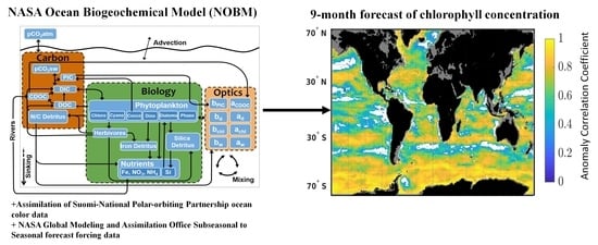
Here, we assess the skills of a seasonal (9-month) forecast of chlorophyll concentration using a dynamical global biogeochemical model. The forcing data used for these forecasts comes from the National Aeronautics and Space Administration (NASA) Global Modeling and Assimilation Office (GMAO) sub-seasonal to seasonal forecast system GEOS-S2S, [
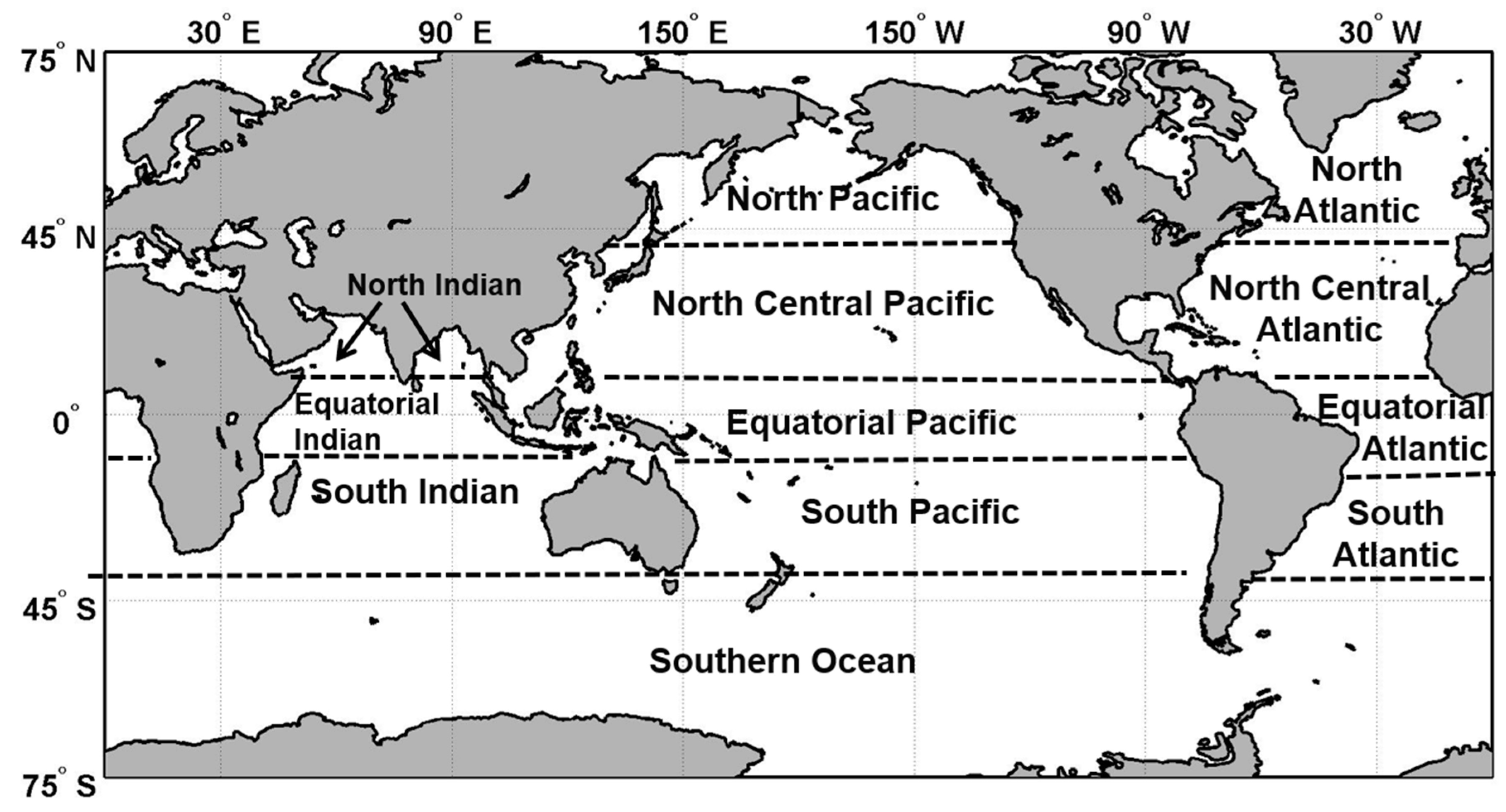
17]). The seasonal forecast timescale is attractive because of the potential to leverage large ongoing modeling efforts and to, in the future, include ocean biogeochemistry alongside climate variables. We first characterize the bias and uncertainties of the system. We then assess the skills of 51 retrospective forecasts of chlorophyll concentration from February 2012 until December 2016 in 12 major oceanographic regions (Figure 1).

2. Materials and Methods

The NASA Ocean Biogeochemical Model (NOBM) is a three-dimensional biogeochemical model of the global ocean coupled with a circulation and radiative model [18]. NOBM has a near-global domain that spans from −84° to 72° latitude at a 1.25° resolution in water deeper than 200 m and contains 6 explicit phytoplankton taxonomic groups (diatoms, cyanobacteria, chlorophytes, dinoflagellates, Phaeocystis sp. and coccolithophores), 3 detritus components (silicate, nitrate/carbon and iron), 4 nutrients (nitrate, silicate, iron and ammonium) and one zooplankton group. The growth of phytoplankton is dependent on total irradiance, nitrogen (nitrate + ammonium), silicate (for diatoms only), iron and temperature see for more details [19]. Surface photosynthetically available radiation is derived from the Ocean-Atmosphere Spectral Irradiance Model (OASIM) [20]). The circulation model used is the Poseidon model [21], a reduced gravity ocean model with 14 layers in quasi-isopycnal coordinates forced by wind stress, sea surface temperature and shortwave radiation [18]. The ocean and atmospheric forcing files used are from the Modern-Era Retrospective analysis for Research and Applications Version 2 from 1979 onward (MERRA-2) [22]. These forcing files are hereafter referred to as transient MERRA-2 and include wind speed and stress, sea surface temperature, shortwave radiation, relative humidity, sea level pressure and sea ice.
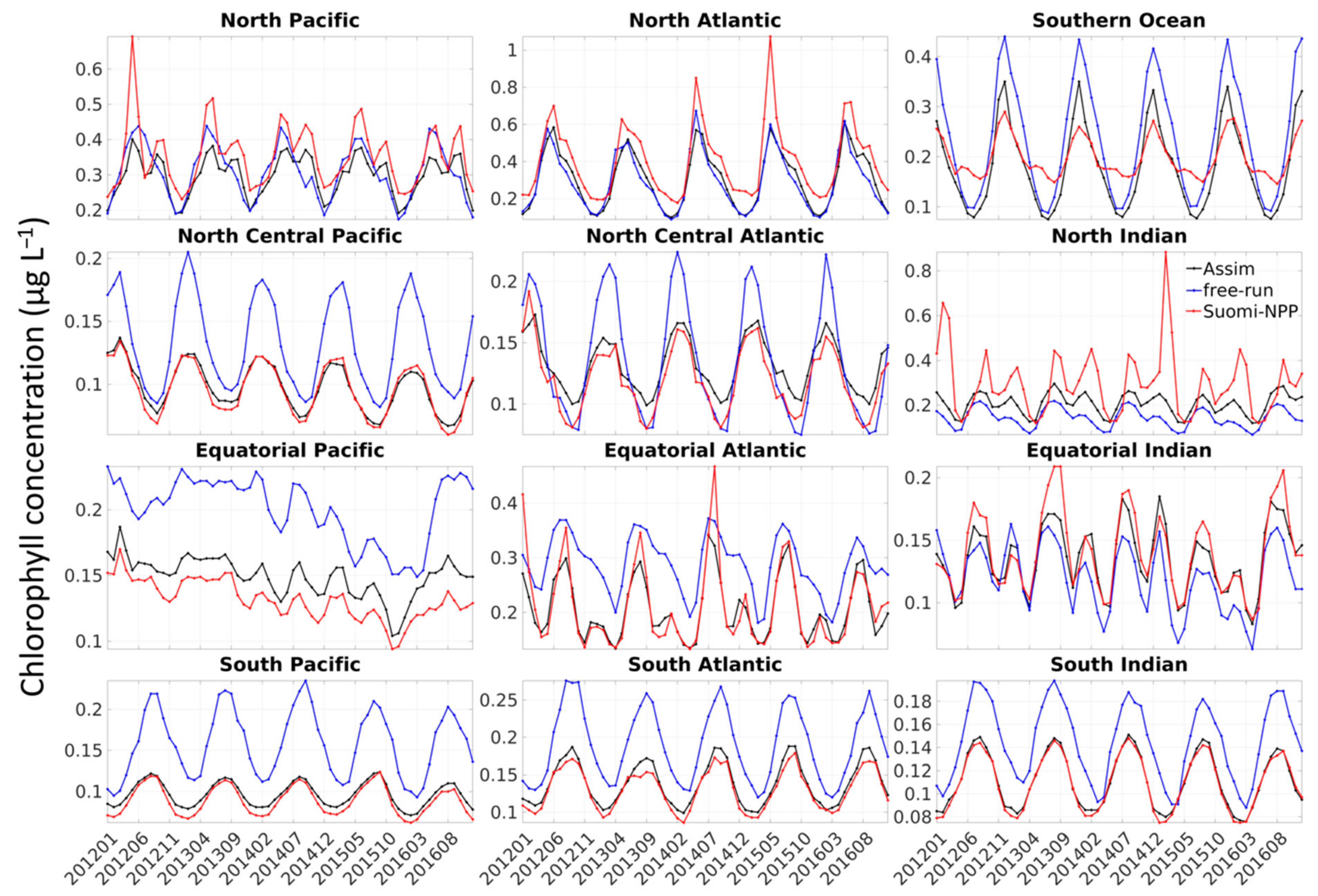
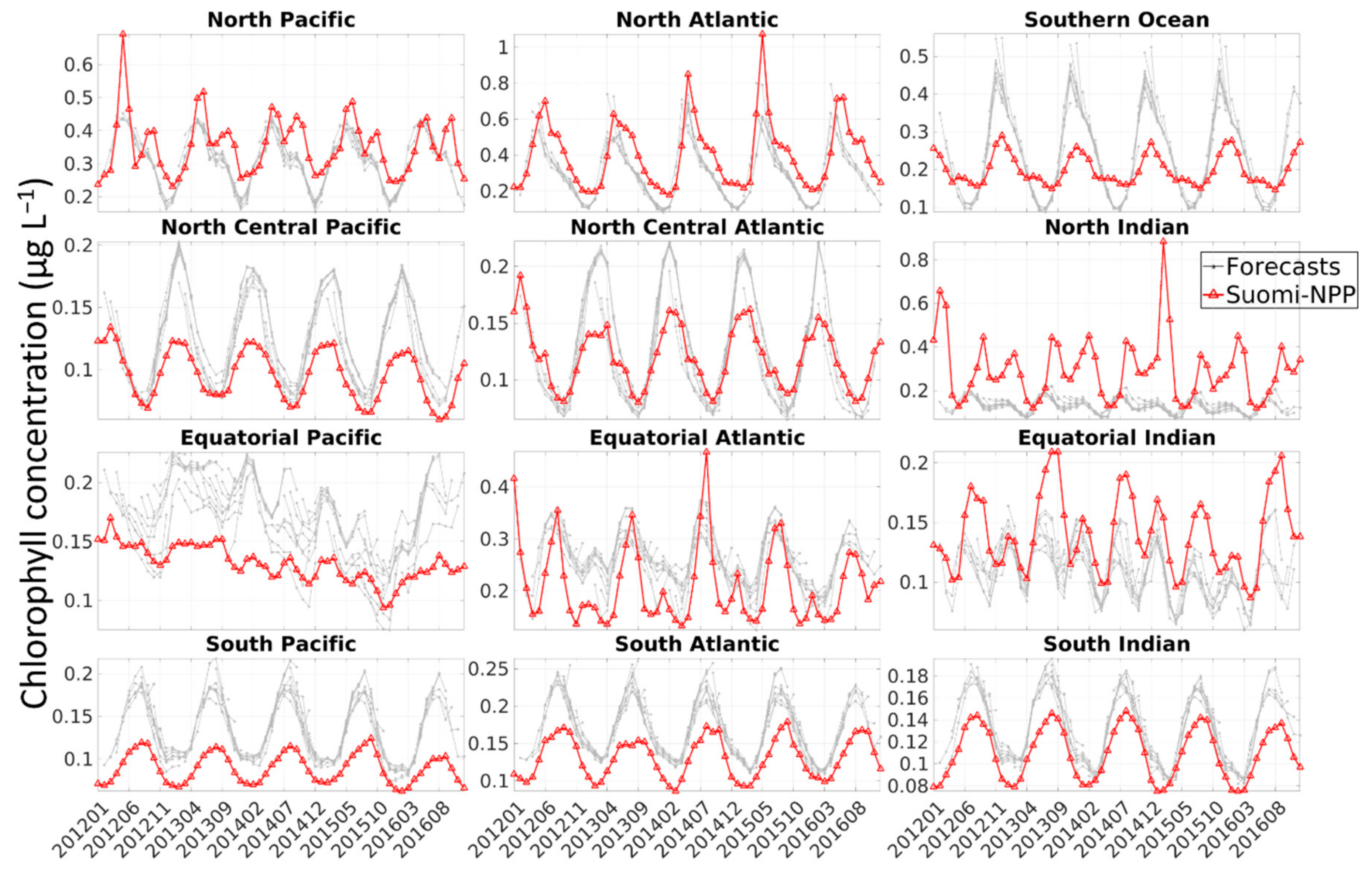
The bias and uncertainties of the system are assessed by comparing the chlorophyll concentration from (1) a free-run model (without data assimilation but using transient MERRA-2 forcing) to Suomi-National Polar-orbiting Partnership (NPP) ocean color data, and (2) the chlorophyll concentration from a run assimilating satellite chlorophyll (using transient MERRA-2 forcing, referred to as ‘the assimilation run’) with those from Suomi-NPP chlorophyll concentration in 12 major oceanographic regions (Figure 1, Table 1). Satellite ocean color chlorophyll concentrations are assimilated from the moderate-resolution imaging spectroradiometer (MODIS-Aqua, 2002–2011) and Suomi-NPP Visible Infrared Imaging Radiometer Suite (VIIRS) (2012–onwards) [23]. The assimilation utilizes the Conditional Relaxation Analysis Method CRAM, [24]), a sequential methodology that adjusts total chlorophyll in the model to satellite data. Individual phytoplankton groups are affected by the assimilation according to their relative abundances in the model. Nutrient concentrations are affected by the assimilation through changes in the nutrient-to-chlorophyll ratios embedded in the model [25]. There are no direct changes to vertical distributions of chlorophyll, phytoplankton or nutrients by the assimilation, but the changes in surface conditions affect the physical environment (light penetration, nutrient availability, vertical gradients) of deeper layers. The Suomi-NPP chlorophyll concentrations were re-gridded to match the model resolution prior to any comparison. Bias is quantified by averaging the monthly percent difference between the chlorophyll concentration from the model (free-run and assimilating run) and that of Suomi-NPP chlorophyll concentration for the period 2012–2016 for each region. The uncertainty is quantified using a correlation coefficient. A statistically significant correlation coefficient is defined as one with a p-value smaller than 0.05.
The initial conditions for the forecasts are produced from a run that uses MERRA-2 forcing and assimilates ocean color chlorophyll concentration. The forcing data used for the forecasts are from the NASA Global Modeling and Assimilation Office (GMAO) sub-seasonal to seasonal forecast system (GEOS-S2S) [17] and include zonal and meridional wind stress, sea surface temperature and shortwave radiation. A total of 51 sets of GMAO forecast data are used to force the 51 monthly biogeochemical forecasts produced here (from February 2012 until December 2016). The skill of the forecasts is assessed using three metrics: (1) the percent difference, (2) the anomaly correlation coefficient (ACC) and (3) the root mean square error (RMSE) between observations and forecasts. These three metrics are commonly used to assess forecasting skills and have been used at many places elsewhere, for example, the Climate Prediction Center (CPC) real-time verification system and World Meteorological Organization (WMO) Standardized Verification System for Long-Range Forecasts (http://www.bom.gov.au/wmo/lrfvs/ (accessed on 29 January 2021)). A total of 51 retrospective forecasts were run, each for a 9-month period. The first forecast started in February 2012 (initialized in January 2012) and the last forecast started in March 2016. The three metrics are calculated using monthly area-weighted mean for each of the regions. Gaps in satellite data resulting from clouds, solar zenith angle, etc., are considered as ‘absent data’ in the calculations. The anomaly correlation coefficient provides information on the linear association between forecast and observations but is insensitive to biases and error in variances. It is calculated as:
A C C = ( p p ¯ ) ( o o ¯ ) ( p p ¯ ) 2 ( o o ¯ ) 2
where p is the model prediction, o is the satellite observation of chlorophyll and p ¯ and o ¯ denote the climatological average for those two values. RMSE measures the magnitude of the error, is sensitive to large values but does not indicate the direction of the error. It is calculated as:
R M S E = 1 N ( p o ) 2
The percent difference between the satellite and the forecasted chlorophyll concentration quantifies the mean error in the forecast. It allows us to assess whether the forecast has a positive or a negative bias. It is calculated as:
Percent   difference = ( p o ) ( p + o 2 ) x   100
All 3 metrics are calculated for each of the 12 major oceanographic regions (Figure 1). Regions are defined as in Conkright et al. [26] with additional equatorial subdivisions in each major ocean from 10 °S to 10° N, and the Southern Ocean is defined as southward of 40°S. Note that previous ensemble simulations with NOBM showed little variability on the chlorophyll forecasts between members, therefore only one member was used to test the forecasting skills of this system. The lack of sensitivity of the systems to various ensembles may be because chlorophyll is relatively insensitive to ensemble variations or because, as noted in Molod et al. [17], the ensemble spread in GEOS-S2S is small.

3. Results

3.1. Bias and Uncertainties in the NASA Ocean Biogeochemical Model

Before assessing the skill of the forecasts, we discuss the performance of the NOBM when forced with reanalysis data. To assess the ability of the system to represent the concentration and variability of chlorophyll in the various regions, we first compared the free-run and assimilation run to the chlorophyll concentration from Suomi-NPP. Chlorophyll concentrations from the free-run were significantly correlated to those from Suomi-NPP in all regions except in the North Indian (R = 0.19, p = 0.15, Figure 2). In the assimilation run, the chlorophyll concentrations in all the regions were significantly correlated to the chlorophyll concentration from Suomi-NPP and were all above or equal to 0.90 (Figure 2). The only exception to this was in the North Indian, where the correlation coefficient was significant but only 0.44.
Out of the 12 regions, the free-run overestimated chlorophyll in 8 of them (6 in the assimilation run, Figure 2). The regions where the system under- or over-estimated chlorophyll were generally the same in the free-run and in the assimilation run. The only exception to this was in the Southern Ocean and Equatorial Atlantic, where the free-run overestimated whereas the assimilation underestimated the chlorophyll concentration. The largest difference between the chlorophyll concentration from the free-run and those from Suomi-NPP was found in the North Indian (61.29%). The assimilation of Suomi-NPP improved the representation of chlorophyll concentration in 9 out of the 12 regions (improvement between 4.12% and 45.61%). Using the free-run, chlorophyll concentrations were within the uncertainties of the satellite data (semi-interquartile range of the Suomi-NPP versus in situ data: 27.9%) in 5 out of the 12 regions analyzed. The assimilation of Suomi-NPP chlorophyll substantially improved this, and all regions except the North Atlantic were within the uncertainty of the Suomi-NPP chlorophyll concentration measurements.
A time-series of chlorophyll concentration from the free-run, assimilation run and Suomi-NPP in each of the regions (Figure 3) further highlights the ability of the free-run to simulate the right seasonal and interannual variability overall, although the magnitude of the chlorophyll concentrations’ variability is not always accurately represented. In the regions identified as overestimating the chlorophyll concentration, the overestimate of chlorophyll concentration was often associated with an overestimate of the seasonal cycle amplitude (e.g., North Central Atlantic and Southern Ocean). In some of these regions, the overestimate was also due to a consistent bias in chlorophyll concentration (e.g., South Pacific, South Atlantic, South Indian, Equatorial Pacific and North Central Pacific). Note that while in the majority of cases the model overestimated chlorophyll concentration, the satellite occasionally observed higher peak values of chlorophyll than the model (e.g., North Pacific in May 2012, North Atlantic in May 2015, North Indian in August 2014), but these were limited to specific events.
Having assessed overall model performance, we can place the performance of forecasts in context. Except in the North Indian, the anomaly correlation coefficients (ACCs) between the chlorophyll concentration from the forecasts and those from Suomi-NPP were significant for most of the lead months (i.e., number of months predicted ahead of time) in all regions (Figure 4).

3.2. Forecast Skills

The Anomaly Correlation Coefficients (ACCs) were higher for the high-latitude regions compared to the equatorial regions (10° S–10° N, Figure 4 and Figure 5, Table 2). All the regions south of 10° S as well as in the North Central Pacific and Atlantic had significant (p < 0.05) ACCs that were always higher than 0.70. This was also true in the North Atlantic (p < 0.05) and the first 4 lead months in the North Pacific (but all lead months were significant). The equatorial regions were characterized by lower ACCs (Figure 4 and Figure 5). Despite the lower ACCs, the forecasted chlorophyll concentrations in the equatorial regions were still significantly correlated to those from Suomi-NPP. This was true for all lead months in the Equatorial Atlantic, all except one month in the Equatorial Indian (lead 4 month) and 6 out of the 9 forecasted months in the Equatorial Pacific. While low-latitude regions had lower ACC, except for the North Indian Ocean, all basins within 40°S–40°N had a RMSE of 0.05 µg chlorophyll (chl) L−1 or less (Table 2). The RMSEs for the basins north and south of 40° (Southern Ocean, North Atlantic and North Pacific) were higher and ranged from 0.05 up to 0.13 µg chl L−1. The RMSEs in the North Indian were among the highest and ranged from 0.13 up to 0.15 µg chl L−1. A linear regression analysis showed that the ACC significantly decreased with the lead month in 6 out of the 12 regions (Antarctic, South Indian, South Pacific, South Atlantic, Equatorial Pacific, North Central Atlantic and North Pacific; Table 2, Figure 4 and Figure 5). Although not significantly, the ACCs were also decreasing in 3 additional regions for a total of 9 regions, where the ACCs were decreasing with lead month.
Overall, most of the forecasted chlorophyll were within the semi-interquartile range (SIQR) of the satellite chlorophyll (27.9 %). This SIQR is based on the uncertainty of the Suomi-NPP chlorophyll measurements. Notable exceptions to this were in the North Indian (all 9 forecast months), North Atlantic (7 out of the 9 forecast months) and South Pacific (all 9 forecast months). A few regions exceeded the SIQR occasionally (3 or less of the forecast lead months): North Central Pacific, Equatorial Atlantic, Equatorial Pacific and South Atlantic. The time series of the chlorophyll concentrations from the various forecasts in comparison with the chlorophyll concentration from Suomi-NPP (Figure 6) highlighted that in a lot of the regions, especially the high latitudes, the seasonal cycle was too pronounced (e.g., North Central Pacific, South Pacific, Southern Ocean).
The percent difference between the chlorophyll concentration from the forecast and that of Suomi-NPP indicated that the largest difference was found in the North Indian (between −57.27% and −71.81% depending on the lead month, Table 2). The South Pacific and North Atlantic also had fairly large differences ranging from 36.64% to 44.73% and −18.40% down to −37.19% respectively, depending on the lead time (Table 2). The regions where the forecasts under- and over-estimated the chlorophyll concentration were identical to those from the comparison between the free-run and from Suomi-NPP (North Atlantic, North Pacific, North Indian and Equatorial Indian). The timeseries of the percent difference (Figure 7) highlighted that although the average for each of the lead months (Table 2) might indicate a consistent over- or under-estimate, the forecasts actually oscillated between over- and under-estimates with a strong seasonal pattern in some regions. In the North Atlantic for example, the timeseries showed that every year in March, the forecast overestimated the chlorophyll concentration by as much as 63.7% and was underestimated in December by as much as −77.4%, while the average percent difference was between −18.40% and −37.19% (Table 2). Only one region had a consistent overestimate throughout the timeseries (South Pacific) and none of the regions had a consistent underestimate.

4. Discussion

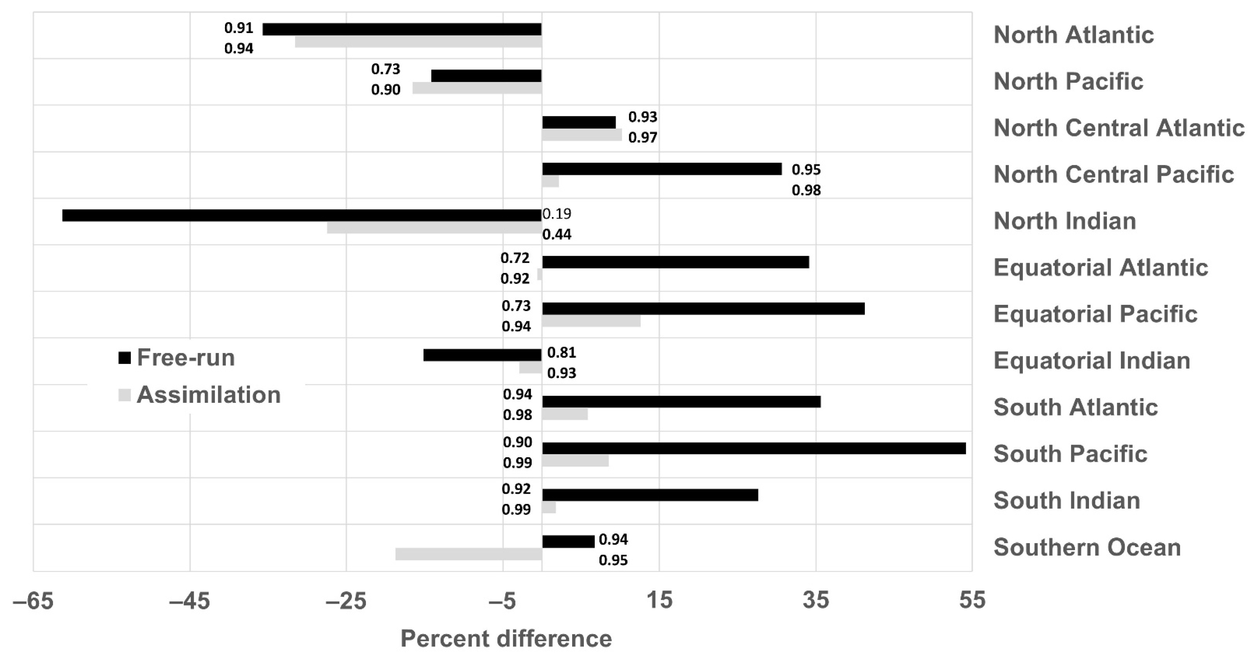
The performance of the system used to generate the forecasts highlighted two important findings: (1) the capability of the model to represent the seasonal phasing (as shown by the high correlation coefficients), although the amplitude is overestimated in several regions (as shown by the RMSE), and (2) the existence of a positive bias in a number of regions. The assimilation decreased the bias in all but 3 regions and allowed the estimate to be within the satellite uncertainties for all regions except the North Atlantic. This is relevant because it means that the assimilation of chlorophyll concentration improves the accuracy of the initial conditions used to generate the forecasts. Skillful forecasts require accurate initialization conditions.
The bias observed was either constant or due to the model simulating a stronger seasonal cycle than the one observed by Suomi-NPP, or both (Figure 3). This suggests that some region-dependent bias correction could be applied to improve the forecasting skills. Model biases are a common characteristic of most seasonal forecasts and can be the result of an imperfect model, a bias in the forcing data, a parametrization requiring fine-tuning or simply the lack or misrepresentation of processes that might play key roles in some regions e.g., [27,28,29]. This is especially true for global models where assumptions must be made that can be too general for local applications. The existence of a stronger seasonal cycle in the model compared to that of satellite data could also be due to the lack of satellite data during specific seasons (i.e., winter) or under some circumstances (e.g., dust storm, fire, etc.). In the high-latitude regions (i.e., Southern Ocean, North Atlantic and North Pacific) for example, the ocean color satellites are known to sample in locations and during periods of favorable phytoplankton growth, thereby producing an overestimate of chlorophyll concentration during certain times of the year [30]. Gregg and Casey [30] estimated that the chlorophyll concentration in the North Pacific, North Atlantic and Southern Ocean was overestimated by 12.8%, 21.7% and 18.4%, respectively. The largest biases were a result of the exclusion of data associated with high solar zenith angle. The bias was lower in the North Pacific and was attributed to the existence of persistent clouds during this season [30]. The overestimate of chlorophyll concentration due to the solar zenith angle and clouds could, for example, explain the lower chlorophyll concentration observed every March in the Southern Ocean, every December–January in the North Atlantic and in summer in the North Pacific in the free-run and assimilation run (Figure 3). This coincides with the annual minima in chlorophyll concentration in the Southern Ocean and North Atlantic and the annual maxima in the North Pacific.
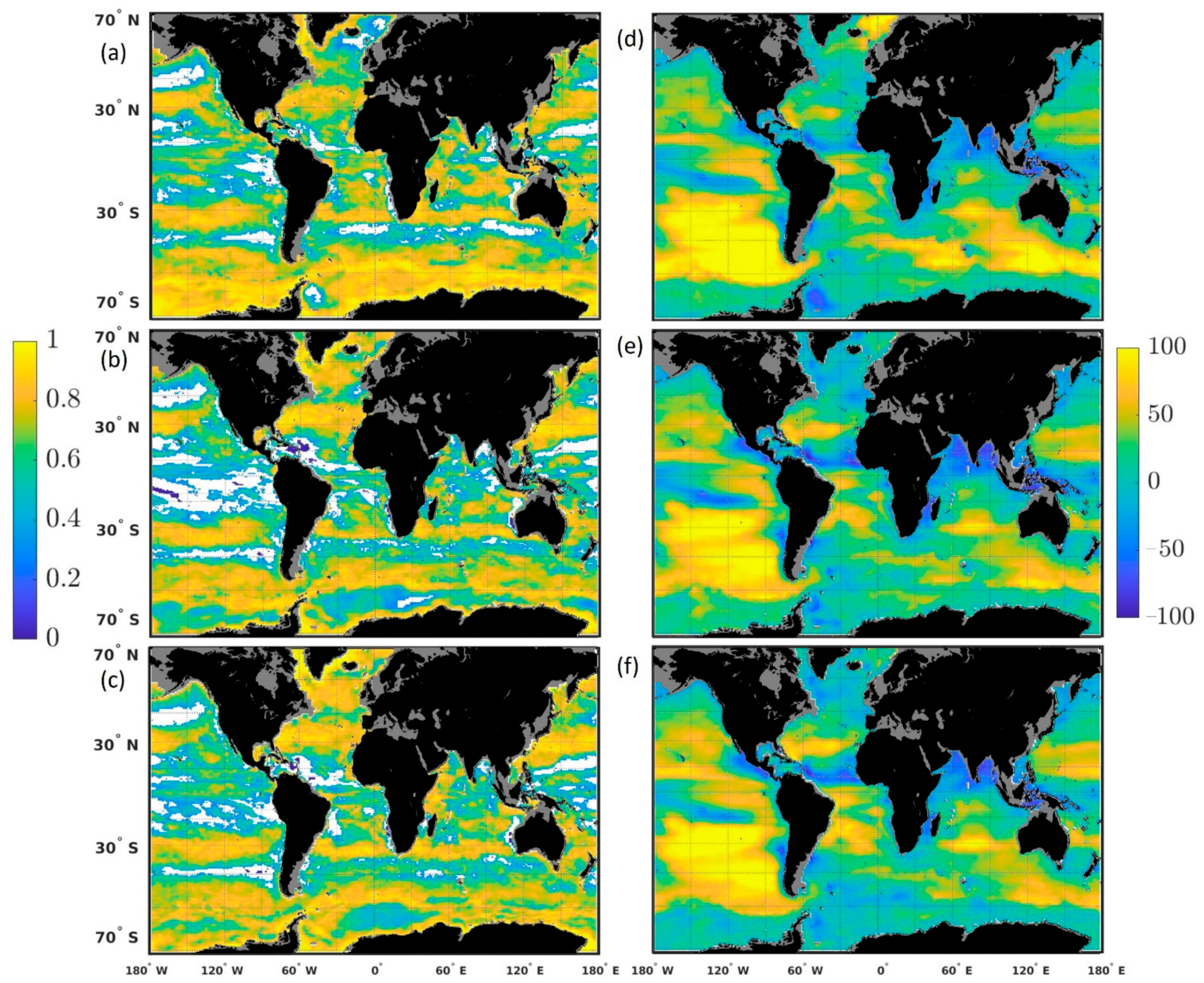
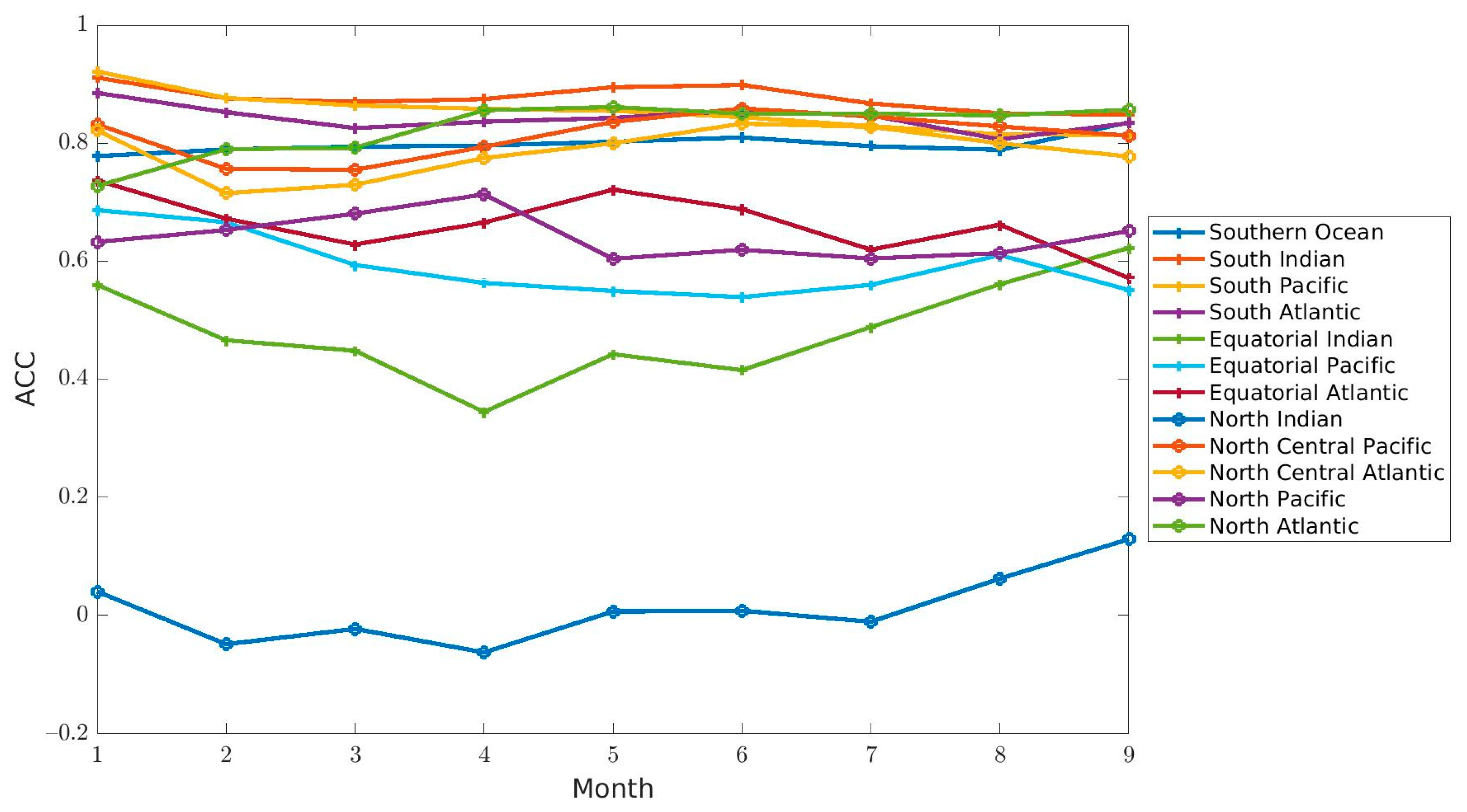
Predictability assesses the ability of observed chlorophyll concentrations to be predicted by a forecast system. The ACCs indicated that the forecasts had the correct variability in chlorophyll concentration for most of the regions (Figure 6, Table 2). As is commonly observed in seasonal forecasts, the skill (as measured here by ACC) degraded with increasing lead month for the majority of regions (9 out of 12, with 6 of them being significant, Table 2, Figure 4. The forecast for all regions except 3 (North Indian, South Pacific, North Atlantic) were within the SIQR of Suomi-NPP, which suggests that a skillful seasonal forecast of chlorophyll at the global scale is possible. The results show that the forecasts rely heavily on the underlying system’s ability to simulate the seasonal cycle. The higher ACCs in the high latitudes were indeed a direct result of the ability of the system to forecast the seasonal cycle rather than the interannual variability. If the ACCs were calculated by removing a seasonal climatology (thereby removing the seasonal cycle) rather than a climatology for the whole period of interest, the ACCs were lower in the high latitudes and higher in the Equatorial regions (Supplementary Table S1). This further demonstrates that the forecast relies heavily on the system’s ability to forecast the seasonal cycle at high latitudes and the interannual variability in the Equatorial regions (Equatorial Pacific and Atlantic). Comparing these forecasts with a model simulation that is forced by a MERRA-2 climatology showed that the ACCs (with seasonality removed, Supplementary Table S1) were always higher for the forecasts than for the simulation that used a MERRA-2 climatological forcing, thereby reinforcing the improved skills of the forecasts over a simple ‘persistence’ simulation. The inherent bias of the system in combination with the potential errors in the predicted forcing conditions contributed to lowering the skills of the forecasting system. Both can be improved in the future to increase the skill of the forecasts. The assimilation of chlorophyll data on the other hand was found to improve the initial conditions of the forecasting system. Finally, the skill of the forecasts was assessed by comparing the chlorophyll concentration with those from the satellite ocean color, which, as indicated above, can have inherent biases related to the existence of clouds, aerosols, high solar zenith angle, etc. These biases in the satellite data can themselves introduce artifacts in the estimates of forecast skill.
Regions with some of the highest ACC also had some of the highest RMSE (i.e., North Atlantic and Southern Ocean). The North Atlantic and Southern Ocean had the right phasing (significant ACCs) but appeared to have the wrong amplitude (high RMSE). The percent difference with the chlorophyll concentration from Suomi-NPP was larger in the North Atlantic than in the Southern Ocean because the forecast was consistently underestimating the chlorophyll here. In the Southern Ocean, the forecasted chlorophyll oscillated between being over- and under-estimated and as a result produced an average difference that was smaller than in the North Atlantic. Another region where the bias was considerable was the South Pacific. Here, the ACCs were significant, the RMSE was low (≤0.03 µg chl L−1) and the percent difference was high (36.64–44.73%). In this region, the forecast had the right variability (ACC) and magnitude (RMSE), but because the system was consistently overestimating chlorophyll, it resulted in a relatively high chlorophyll overestimate. Note that while regions were defined in this study, a spatial distribution of the correlation and percent difference highlighted the relative consistency in patterns of highs and lows depending on the lead time of the forecast (Figure 5). Furthermore, the percent difference is affected by the concentration of chlorophyll. This explains the large percent difference observed, for example, in the South Pacific, where chlorophyll concentrations are relatively low compared to other regions and results in large percentage difference when compared to Suomi-NPP. Note that the ACCs are not affected by this since they are based on anomalies.
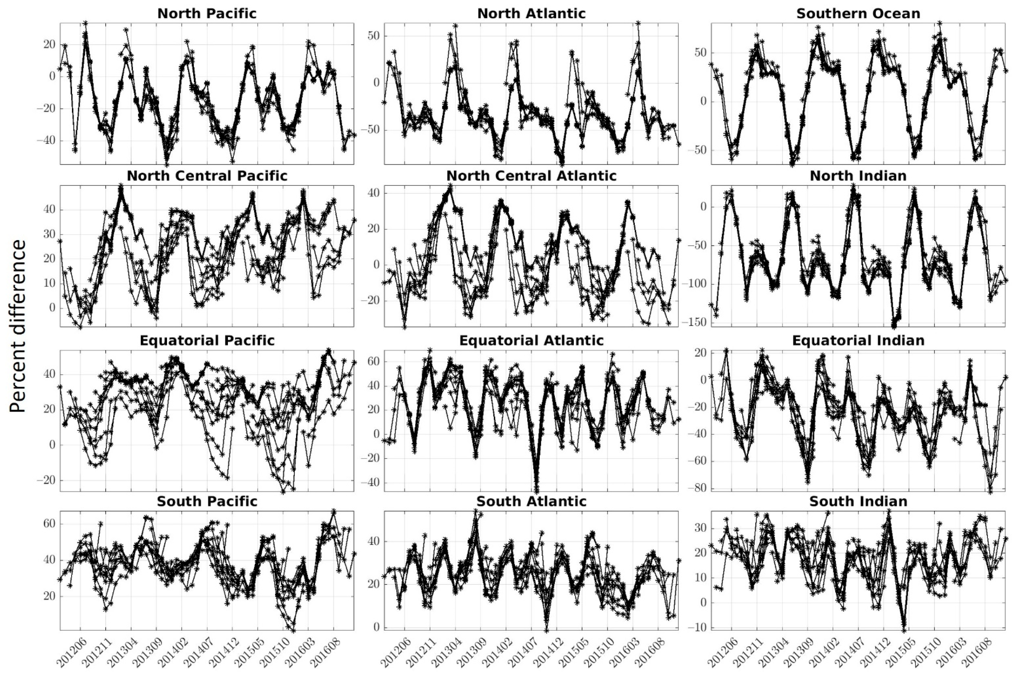
Finally, the timeseries representing the percent difference between the chlorophyll from the forecasts versus that of Suomi-NPP further highlights the seasonality of the error (Figure 7). Depending on the regions, there is a pattern of increasing and decreasing bias in our forecast, with either an annual (e.g., North Pacific, Figure 7) or bi-annual cycle (e.g., South Indian). Chlorophyll concentration were consistently (except for a few instances) overestimated in only a few regions (South Atlantic, South Pacific, North Central Pacific). The chlorophyll concentration was not underestimated throughout the entire timeseries in any of the regions (although the chlorophyll concentrations in the North and Equatorial Indian are mostly under-estimated).
This study shows the potential to forecast biogeochemical parameters at the global scale using a dynamical model. The results highlight several potential areas of improvements needed in the system, the most obvious one being to correct the existing bias in the system. This paper represents the first step towards developing a set of corrections that could be either region-dependent or applied at the pixel level and that would further improve the forecasts. The model uncertainty could also be accounted for by using some stochastic parametrization at the sub-grid level, such as the one used by the European Centre for Medium-Range Weather Forecasts [31]. This forecasting system could also benefit from being integrated in a fully coupled system where the forecast of biogeochemistry can in turn affect other parameters such as the temperature of the oceans. This need to integrate the various components in forecasting systems (including biogeochemistry) has already been highlighted by Ford et al. [32]. Finally, the current system does not cover waters that are shallower than 200 m, and this of course limits the potential applications of such of forecasting system but can also decrease the apparent skills of the forecasts since the model does not include the potential lateral transport of high chlorophyll, dissolved sediments and nutrients from coastal waters. The pelagic pixels adjacent to these coastal pixels could therefore see an increase in nutrients and chlorophyll concentration once the model does include coastal waters.
The development of the biogeochemical forecast system described here can improve our capabilities in assessing the extent of the effects that climate variability, such as ENSO, have on ocean biogeochemistry and the recruitment of higher trophic levels. In the last two decades, we have witnessed the development of two major El Niño events that had considerable impacts on both land and ocean conditions. The 1997–1998 El Niño was particularly devastating for the ocean resources and led to the collapse of several fisheries and dramatic socio-economic repercussions for countries such as Peru. If the effects that this type of event had on fisheries had been predicted, the damages could have been reduced by adapting fisheries strategies. Assessing the factors that influence the predictability of ocean biogeochemistry at sub-seasonal and seasonal scales will improve the forecast capabilities at longer timescales and provide information about the changes in the ocean–atmosphere carbon cycle. Since phytoplankton and other biogeochemical constituents are key contributors to ocean heat transfer e.g., [33,34], this effort can potentially also improve forecasts of ocean physical variability, including the timing and magnitude of ENSO events, as well as other regions such as the tropical Indian Ocean, the northwest Pacific (e.g., the “blob”) and the Arctic, as well as atmospheric events, such as hurricane, that depend heavily on ocean heat content. A forecast of the biogeochemical conditions could also help in designing sampling plans, support design simulation experiments where various field sampling strategies could be tested to improve the efficiency of the field campaigns and provide a representative sampling of existing conditions. Finally, predicting the dynamic of the phytoplankton population can also be advantageous for local applications as well. The increase in frequency of Harmful Algal Blooms (HABs) in specific areas is the subject of increasing attention in the last decades as a result of the increase in their frequency and intensity. While the current system does not include HAB species and is most likely currently too coarse for such applications, it represents a first step towards the ability to forecast such HABs at the global scale.

5. Conclusions

This paper showed the skills of a 9-month forecast of chlorophyll concentration at the global scale. The skills were found to be highly dependent on the ability of the underlying system to produce the right seasonal variability. Existing biases in this system were reflected in the forecasting system. The use of ocean color data assimilation to produce initial conditions provided an improvement to the system. While further fine-tuning to the system is necessary, the system’s skills show that such a biogeochemical forecasting system could be integrated in a fully coupled system, where the forecast of biogeochemistry can in turn affect other parameters, such as the temperature of the oceans. The system presented here has numerous applications once these improvements are made and could be beneficial to several societal applications.

Supplementary Materials

The following are available online at https://www.mdpi.com/2072-4292/13/6/1051/s1, Table S1: Anomaly correlation coefficient with seasonal cycle removed (first line), Root Mean Square Error (second line) and percent chlorophyll concentration difference between the forecast and Suomi-NPP (third line) for each of the regions and for the various lead-month (column 1 through 9).

Author Contributions

Conceptualization, C.S.R.; methodology, C.S.R., W.W.G., L.O.; validation, C.S.R., W.W.G., L.O.; formal analysis, C.S.R.; investigation, C.S.R.; resources, C.S.R., W.W.G., L.O.; data curation, C.S.R.; writing—original draft preparation, C.S.R.; writing—review and editing, C.S.R., W.W.G., L.O.; visualization, C.S.R.; supervision, C.S.R.; project administration, C.S.R.; funding acquisition, C.S.R., L.O. All authors have read and agreed to the published version of the manuscript.

Funding

This paper was funded by the NASA Modeling, Analysis and Prediction Program (80NSSC17K0268), NASA EXPORTS (NNX16AR51G) and the NASA Interdisciplinary Research in Earth Science Program (16-IDS16-0039).

Institutional Review Board Statement

Not applicable.

Informed Consent Statement

Not applicable.

Data Availability Statement

The assimilated NASA Ocean Biogeochemical Model data are available on the NASA Giovanni portal (https://giovanni.sci.gsfc.nasa.gov/giovanni/#service=TmAvMp&starttime=&endtime=&variableFacets=dataProductPlatformInstrument%3ANOBM%20Model%3B) and the following ftp: https://gmao.gsfc.nasa.gov/gmaoftp/NOBM/monthly/ (accessed on 29 January 2021). The forecasted data are available on request from the corresponding author.

Acknowledgments

We thank the NASA Ocean Ecology Laboratory for providing the satellite chlorophyll data and the NASA Center for Climate Simulation for computational support. The GEOS-5 data used in this study/project have been provided by the Global Modeling and Assimilation Office (GMAO) at NASA Goddard Space Flight Center through the online data portal in the NASA Center for Climate Simulation.

Conflicts of Interest

The authors declare no conflict of interest.

References

  1. Cole, J. Environmental conditions, satellite imagery, and clupeoid recruitment in the northern Benguela upwelling system. Fish. Oceanogr. 1999, 8, 25–38. [Google Scholar] [CrossRef]
  2. Zagaglia, C.R.; Lorenzzetti, J.A.; Stech, J.L. Remote sensing data and longline catches of yellowfin tuna (Thunnus albacares) in the equatorial Atlantic. Remote Sens. Environ. 2004, 93, 267–281. [Google Scholar] [CrossRef]
  3. Bigelow, K.A.; Maunder, M.N. Does habitat or depth influence catch rates of pelagic species? Can. J. Fish. Aquat. Sci. 2007, 64, 1581–1594. [Google Scholar] [CrossRef] [Green Version]
  4. Herron, R.C.; Leming, T.D.; Li, J. Satellite-detected fronts and butterfish aggregations in the northeastern Gulf of Mexico. Cont. Shelf Res. 1989, 9, 569–588. [Google Scholar] [CrossRef]
  5. Park, J.-Y.; Stock, C.A.; Dunne, J.P.; Yang, X.; Rosati, A. Seasonal to multiannual marine ecosystem prediction with a global Earth system model. Science 2019, 365, 284–288. [Google Scholar] [CrossRef]
  6. Siedlecki, S.A.; Kaplan, I.C.; Hermann, A.J.; Nguyen, T.T.; Bond, N.A.; Newton, J.A.; Williams, G.D.; Peterson, W.T.; Alin, S.R.; Feely, R.A. Experiments with seasonal forecasts of ocean conditions for the northern region of the California Current upwelling system. Sci. Rep. 2016, 6, 1–18. [Google Scholar] [CrossRef] [PubMed] [Green Version]
  7. Séférian, R.; Bopp, L.; Gehlen, M.; Swingedouw, D.; Mignot, J.; Guilyardi, E.; Servonnat, J. Multiyear predictability of tropical marine productivity. Proc. Natl. Acad. Sci. USA 2014, 111, 11646–11651. [Google Scholar] [CrossRef] [Green Version]
  8. Platt, T. The concept of energy efficiency in primary production. Limnol. Oceanogr. 1969, 14, 653–659. [Google Scholar] [CrossRef]
  9. Murtugudde, R.; Beauchamp, J.; McClain, C.R.; Lewis, M.; Busalacchi, A.J. Effects of penetrative radiation on the upper tropical ocean circulation. J. Clim. 2002, 15, 470–486. [Google Scholar] [CrossRef]
  10. Wetzel, P.; Maier-Reimer, E.; Botzet, M.; Jungclaus, J.; Keenlyside, N.; Latif, M. Effects of ocean biology on the penetrative radiation in a coupled climate model. J. Clim. 2006, 19, 3973–3987. [Google Scholar] [CrossRef] [Green Version]
  11. Park, J.-Y.; Kug, J.-S.; Bader, J.; Rolph, R.; Kwon, M. Amplified Arctic warming by phytoplankton under greenhouse warming. Proc. Natl. Acad. Sci. USA 2015, 112, 5921–5926. [Google Scholar] [CrossRef] [Green Version]
  12. Nakamoto, S.; Kumar, S.P.; Oberhuber, J.; Ishizaka, J.; Muneyama, K.; Frouin, R. Response of the equatorial Pacific to chlorophyll pigment in a mixed layer isopycnal ocean general circulation model. Geophys. Res. Lett. 2001, 28, 2021–2024. [Google Scholar] [CrossRef]
  13. Lengaigne, M.; Madec, G.; Bopp, L.; Menkes, C.; Aumont, O.; Cadule, P. Bio-physical feedbacks in the Arctic Ocean using an Earth system model. Geophys. Res. Lett. 2009, 36. [Google Scholar] [CrossRef]
  14. Manizza, M.; Le Quéré, C.; Watson, A.J.; Buitenhuis, E.T. Bio-optical feedbacks among phytoplankton, upper ocean physics and sea-ice in a global model. Geophys. Res. Lett. 2005, 32. [Google Scholar] [CrossRef]
  15. Friedlingstein, P.; Jones, M.; O’sullivan, M.; Andrew, R.; Hauck, J.; Peters, G.; Peters, W.; Pongratz, J.; Sitch, S.; Le Quéré, C. Global carbon budget 2019. Earth Syst. Sci. Data 2019, 11, 1783–1838. [Google Scholar] [CrossRef] [Green Version]
  16. Lovenduski, N.S.; Yeager, S.G.; Lindsay, K.; Long, M.C. Predicting near-term variability in ocean carbon uptake. Earth Syst. Dyn. 2019, 10, 45–57. [Google Scholar] [CrossRef] [Green Version]
  17. Molod, A.; Hackert, E.; Vikhliaev, Y.; Zhao, B.; Barahona, D.; Vernieres, G.; Borovikov, A.; Kovach, R.M.; Marshak, J.; Schubert, S. GEOS-S2S Version 2: The GMAO High-Resolution Coupled Model and Assimilation System for Seasonal Prediction. J. Geophys. Res. Atmos. 2020, 125, e2019JD031767. [Google Scholar] [CrossRef]
  18. Gregg, W.W.; Casey, N.W. Modeling coccolithophores in the global oceans. Deep Sea Res. Part. Ii 2007, 54, 447–477. [Google Scholar] [CrossRef]
  19. Rousseaux, C.S.; Gregg, W.W. Recent decadal trends in global phytoplankton composition. Glob. Biogeochem. Cycles 2015, 29, 1674–1688. [Google Scholar] [CrossRef] [Green Version]
  20. Gregg, W.W.; Casey, N.W. Skill assessment of a spectral ocean-atmosphere radiative model. J. Mar. Syst. 2009, 76, 49–63. [Google Scholar] [CrossRef]
  21. Schopf, P.S.; Loughe, A. A reduced-gravity isopycnal ocean model: Hindcasts of El Niño. Mon. Weather Rev. 1995, 123, 2839–2863. [Google Scholar] [CrossRef] [Green Version]
  22. Rienecker, M.M.; Suarez, M.J.; Gelaro, R.; Todling, R.; Bacmeister, J.; Liu, E.; Bosilovich, M.G.; Schubert, S.D.; Takacs, L.; Kim, G.-K. MERRA: NASA’s Modern-Era Retrospective Analysis for Research and Applications. J. Clim. 2011, 24, 3624–3648. [Google Scholar] [CrossRef]
  23. Gregg, W.W.; Rousseaux, C.S. Decadal Trends in Global Pelagic Ocean Chlorophyll: A New Assessment Combining Multiple Satellites, In Situ Data, and Models. J. Geophys. Res. 2014, 119. [Google Scholar] [CrossRef] [Green Version]
  24. Gregg, W.W. Assimilation of SeaWiFS ocean chlorophyll data into a three-dimensional global ocean model. J. Mar. Syst. 2008, 69, 205–225. [Google Scholar] [CrossRef] [Green Version]
  25. Rousseaux, C.S.; Gregg, W.W. Climate variability and phytoplankton composition in the Pacific Ocean. J. Geophys. Res. 2012, 117, C10006. [Google Scholar] [CrossRef]
  26. Conkright, M.E.; Levitus, S.; Boyer, T.P. World Ocean. Atlas, Vol. 1: Nutrients, NOAA Atlas NESDIS 1, 150pp; DIANE Publishing: Darby, PA, USA, 1994. [Google Scholar]
  27. Scaife, A.A.; Woollings, T.; Knight, J.; Martin, G.; Hinton, T. Atmospheric blocking and mean biases in climate models. J. Clim. 2010, 23, 6143–6152. [Google Scholar] [CrossRef] [Green Version]
  28. Becker, E.; den Dool, H.; Zhang, Q. Predictability and forecast skill in NMME. J. Clim. 2014, 27, 5891–5906. [Google Scholar] [CrossRef]
  29. Smith, T.M.; Livezey, R.E. GCM systematic error correction and specification of the seasonal mean Pacific–North America region atmosphere from global SSTs. J. Clim. 1999, 12, 273–288. [Google Scholar] [CrossRef]
  30. Gregg, W.W.; Casey, N.W. Sampling biases in MODIS and SeaWiFS ocean chlorophyll data. Remote Sens. Environ. 2007, 111, 25–35. [Google Scholar] [CrossRef] [Green Version]
  31. Buizza, R.; Milleer, M.; Palmer, T. Stochastic representation of model uncertainties in the ECMWF ensemble prediction system. Q. J. R. Meteorol. Soc. 1999, 125, 2887–2908. [Google Scholar] [CrossRef]
  32. Ford, D.; Key, S.; McEwan, R.; Totterdell, I.; Gehlen, M. Marine biogeochemical modelling and data assimilation for operational forecasting, reanalysis, and climate research. New Front. Oper. Oceanogr. 2018, 625–652. [Google Scholar]
  33. Lewis, M.R.; Cullen, J.J.; Platt, T. Phytoplankton and thermal structure in the upper ocean: Consequences of nonuniformity in chlorophyll profile. J. Geophys. Res. 1983, 88, 2565–2570. [Google Scholar] [CrossRef]
  34. Anderson, W.; Gnanadesikan, A.; Hallberg, R.; Dunne, J.; Samuels, B. Impact of ocean color on the maintenance of the Pacific Cold Tongue. Geophys. Res. Lett. 2007, 34. [Google Scholar] [CrossRef] [Green Version]
Figure 1. Delineation of the 12 oceanographic regions.
Remotesensing 13 01051 g001
Figure 2. Percent difference between the chlorophyll concentration from the free-run/assimilation run and those from Suomi- National Polar-orbiting Partnership (NPP) for the period from January 2012 until December 2016. Correlation coefficients are located next to the corresponding bars and bold indicates p < 0.05.
Remotesensing 13 01051 g002
Figure 3. Chlorophyll concentration for the 12 regions from the assimilation run (assimilating Suomi-NPP, black), free-run (blue), Suomi-NPP chlorophyll concentration (red) for the period from January 2012 until December 2016.
Remotesensing 13 01051 g003
Figure 4. Anomaly Correlation Coefficient (ACC) for the 12 regions for the 9-lead month.
Remotesensing 13 01051 g004
Figure 5. Correlation coefficient between the average lead 1 (a), lead 5 (b) and lead 9 (c) forecasts and the corresponding Suomi-NPP chlorophyll concentration (column 1, 5 and 9 in Table 2). Percent difference between the average lead 1 (d), lead 5 (e) and lead 9 (f) forecasts and the corresponding Suomi-NPP chlorophyll concentration. The white spaces indicate a non-significant correlation (p > 0.05). Grey space indicates the areas not covered by the model (shallower than 200 m).
Remotesensing 13 01051 g005
Figure 6. Chlorophyll concentration (µg L−1) from the 51 different forecasts (grey lines), and Suomi-NPP chlorophyll (red triangle). Each of the 51 retrospective forecasts were run for a 9-month period. The first forecast started in February 2012 (initialized in January 2012) and the last forecast started in March 2016.
Remotesensing 13 01051 g006
Figure 7. Percent difference between the chlorophyll concentrations from the forecasts and those from Suomi-NPP. Each of the 51 retrospective forecasts were run for a 9-month period. The first forecast started in February 2012 (initialized in January 2012) and the last forecast started in March 2016.
Remotesensing 13 01051 g007
Table 1. Summary of the various simulations as well as their forcing data and whether ocean color data was assimilated or not. MERRA-2: Modern-Era Retrospective analysis for Research and Applications, GMAO-S2S: Global Modeling and Assimilation Office-Subseasonal to Seasonal forecasts.
PurposeNameForcingAssimilation of Ocean Color Data?
System PerformanceFree runMERRA-2No
Assimilation run MERRA-2Yes
Forecast initial conditionsAssimilation runMERRA-2Yes
ForecastsFree runGMAO-S2S forecastNo
Table 2. Anomaly Correlation Coefficient (ACC) (first line), root mean square error (RMSE) (µg chlorophyll (chl) L−1, second line) and percent chlorophyll concentration difference between the forecast and Suomi-NPP (third line) for each of the regions and for the various lead-month (column 1 through 9). ACCs in bold indicate that the results were significant (p < 0.05).
123456789
North Atlantic0.790.830.760.790.790.770.770.770.80
0.120.090.120.120.120.110.110.110.10
−18.40−26.80−35.26−37.19−36.81−36.35−35.94−35.30−35.48
North Pacific0.700.720.730.750.610.590.500.480.54
0.070.060.060.060.050.050.060.070.07
−10.36−12.42−14.79−15.72−15.13−14.90−15.56−16.42−16.28
North Central Atlantic0.860.800.780.800.800.790.760.740.75
0.030.020.020.010.010.020.020.030.03
7.420.860.261.563.244.225.777.709.37
North Central Pacific0.820.790.780.790.820.840.800.780.80
0.020.020.010.010.010.010.010.020.02
23.2420.7021.7522.0823.2625.4527.3629.5930.34
North Indian0.11−0.08−0.10−0.080.040.120.090.050.02
0.150.150.140.140.140.130.140.140.14
−57.27−62.13−61.71−63.35−68.02−70.93−71.81−70.27−68.42
Equatorial Atlantic0.720.670.640.670.720.750.670.650.56
0.050.050.050.050.050.050.050.050.05
26.7521.0222.3825.3826.6027.3828.3529.5034.26
Equatorial Pacific0.460.430.340.320.330.280.240.290.09
0.020.020.020.020.020.020.020.020.03
30.0324.5923.6723.0722.6522.6323.8726.6234.37
Equatorial Indian0.630.380.290.260.440.450.500.520.49
0.020.030.030.030.030.030.030.030.03
−18.89−26.78−24.95−24.45−26.14−25.75−25.43−21.87−16.19
South Atlantic0.880.850.840.830.810.820.790.740.83
0.020.020.010.010.010.010.020.020.03
26.5623.9425.3024.8124.4023.9223.9423.9830.46
South Pacific0.930.900.870.860.850.810.750.740.79
0.030.020.020.010.010.010.020.030.03
38.3836.8736.6437.0037.1736.9837.2437.9944.73
South Indian0.910.880.870.850.850.850.790.800.85
0.020.010.010.010.010.010.010.020.02
21.1117.3017.0216.0916.0816.5616.6217.9522.35
Southern Ocean0.810.800.780.780.780.760.700.700.78
0.130.080.070.060.060.060.070.100.10
21.7110.867.195.866.837.368.109.296.45
Publisher’s Note: MDPI stays neutral with regard to jurisdictional claims in published maps and institutional affiliations.

