Semantically Derived Geometric Constraints for MVS Reconstruction of Textureless Areas

Abstract

Conventional multi-view stereo (MVS) approaches based on photo-consistency measures are generally robust, yet often fail in calculating valid depth pixel estimates in low textured areas of the scene. In this study, a novel approach is proposed to tackle this challenge by leveraging semantic priors into a PatchMatch-based MVS in order to increase confidence and support depth and normal map estimation. Semantic class labels on image pixels are used to impose class-specific geometric constraints during multiview stereo, optimising the depth estimation on weakly supported, textureless areas, commonly present in urban scenarios of building facades, indoor scenes, or aerial datasets. Detecting dominant shapes, e.g., planes, with RANSAC, an adjusted cost function is introduced that combines and weighs both photometric and semantic scores propagating, thus, more accurate depth estimates. Being adaptive, it fills in apparent information gaps and smoothing local roughness in problematic regions while at the same time preserves important details. Experiments on benchmark and custom datasets demonstrate the effectiveness of the presented approach.

1. Introduction

Multi-View Stereo (MVS) algorithms address the problem of generating a complete and dense 3D representation of the scene, given the camera calibration parameters and poses in the 3D space commonly obtained by Structure from Motion (SfM) pipelines. Such procedures have become a common practice for numerous applications that span from industrial and monitoring scenarios to cultural heritage, city mapping and localization, or autonomous navigation.

Seitz et al. [1] proposed a taxonomy based on which, a MVS pipeline may refer to feature point growing-based methods, voxel-based methods, surface evolution-based methods and depth map merging-based methods. The latter techniques, where depth maps are fused together into a point cloud or a volumetric representation of the scene, are widely used under large scale or high precision applications due to their efficiency and scalability [2,3].

Among the various depth estimation approaches such as semi-global matching [4] or the recent learning solutions [5,6,7], PatchMatch-based [8,9,10] methods have been proven to work efficiently, especially when it comes to accurate depth estimation of slanted surfaces due to the usage of support windows to eliminate fronto-parallel bias. PatchMatch for depth estimation, motivated by the coherent natural structure of the images, applies iterative spatial propagation of the estimated depth in a sequential [11] or diffusion-like fashion [12]. As with other depth estimation methods, PatchMatch relies on photo-consistency measures such as the Normalized Cross Correlation (NCC) and thus strongly depends on the texture variation of the pixel’s neighbourhood. Eventually these algorithms often fail to reconstruct correctly the depth in the areas of low texture, as photo-consistency measures alone are not robust enough to tackle depth inconsistencies and matching ambiguities. Such textureless areas lacking reliable data for depth estimation are also called “weakly supported” regions [13] and are generally present in urban scenes of smooth, homogeneous building facades or indoor scenarios surfaces. To overcome this barrier, higher-level scene understanding constraints have to be introduced [3] to promote the propagation of correct depth estimates between adjacent pixels.

In the latest years, machine and deep learning algorithms have gained popularity in various fields of data science due to the increase of computational power and the amount of available data. Particularly while tackling scene understanding problems such as image classification, segmentation and object detection, the use of Convolutional Neural Networks (CNNs) has become common practise [14,15,16]. Scene understanding information in the form of semantic annotations has been used for image orientation (pose estimation) [17], dense point cloud generation [18] or mesh refinement [19,20,21].

In this article, we present a new framework in which semantic information is used to support MVS and improve 3D point cloud accuracy. In particular, constraints derived from semantically segmented images are used to imply additional class-specific shape priors during cost computation in PatchMatch MVS (Figure 1). The idea is based on the fact that semantics can successfully indicate textureless areas derived by the class label of the scene (e.g., “wall”) where frequently depth miscalculations occur. Geometric constraints can be assigned to these regions to fill in information gaps, while object boundaries and depth details are preserved. Standard PatchMatch approaches make however a priori regularization assumptions to ensure smoothness, yet additional geometric constraints can be implied directly e.g., local planarity [22,23,24]. Instead, we formulate geometric constraints based on semantic priors and benefit from the class-specific geometric properties. RANSAC planes are detected for all dominant surfaces presented in the scene e.g., under “wall”, “floor” or “building” label which we assume are planar. A new weighted cost function is introduced to integrate depth priors and texture information of pixel neighborhood. This achieves gap filling and local roughness smoothing in textureless areas while promoting the confidence of photo-consistency measure on highly textureless ones. The method exploits so far planar regions but can easily be extended to other shapes. Our framework is validated over the ETH3D benchmark dataset and other custom sequences. Moreover, per-pixel labels are projected into the 3D point cloud to generate semantically enriched representations.

The rest of the article is organized as follows: Section 2 introduces a review of the state of the art methods on image segmentation and MVS algorithms, as well as their potential integration; Section 3 outlines the basics of the used PatchMatch MVS algorithm and the respective notation; Section 4 presents our proposed methodology, namely the prior generation and the new cost function; Experiments on various datasets are detailed in Section 5, followed by discussion of the results (Section 6) and Conclusions (Section 7).

2. Related Work

This study proposes a method bridging diverse research fields, thus we hereafter review the respective literature.

2.1. Image Segmentation

Semantic segmentation, i.e., the assignment of every pixel of the image to a semantically meaningful class label, in the past was performed using handcrafted features and flat classifiers [25,26,27]. In the deep learning era, CNNs have enjoyed great success as they tend to outperform other hand-crafted methods in efficiency and accuracy [28]. Originally introduced in the 1980s, yet gained popularity when AlexNet, the seminal work of Krizhevsky et al. [29], won the ImageNet Large-Scale Visual Recognition Challenge (ILSVRC). Thereafter, other CNN architectures are being exploited for image tasks, such as VGG [30], ResNet [31], GoogleNet [32] and Inception [33,34] or DenseNet [35]. Long et al. [36] proposed a Fully Convolutional Network (FCN) i.e., a network with only convolutional layers that can manage arbitrary sized images. Commonly used FCN architectures for image segmentation are DeepLab [14], SegNet [15] and Enet [16]. A detailed overview of the image segmentation models is presented in [37].

Other than a standalone research task, semantic segmentation is used to support various pipelines such as navigation and obstacle avoidance. Thus, an extensive bibliography on semantic segmentation applications exists, especially on urban street scenes, towards the complete scene understanding for autonomous driving purposes. Indeed, several benchmark datasets of real and synthetic data for semantics and 3D reconstruction info have been introduced such as CamVid [38], Rue-Monge2014 [39], CityScapes [40]. Considerable work has been done lately on semantic RGB-D datasets such as the Stanford 2D-3D semantics dataset [41], SUN RGBD [42], NYU Depth v2 [43], SceneNet RGB-D [44]. In aerial scenarios, the UDD [45] and the UAVid [46] dataset series are released to test the performance of various segmentation models over drone image sets of urban areas and the ISPRS 2D semantic labelling dataset provides very high resolution orthophotos with semantic classes for remote sesning applications [47].

2.2. Semantic 3D Reconstruction

Several works couple 3D reconstruction and semantics. They either refer to joint segmentation and reconstruction optimization for multi-view [48,49] and monocular setups using conditional random fields [50] or to the use of depth maps to support 2D segmentation [51]. In the volumetric representation domain, Häne et al. [19,52] proposed to tackle joint volumetric 3D with semantics in multi-view scenarios with variational optimization, while Savinov et al. [53] applied a ray potential computation method in a semantic context. Blaha et al. [21,54], inspired by [19], enabled semantic segmentation and volumetric reconstruction in a joint fashion for surface refinement of large scale scenes, updating shapes and labels simultaneously. Similarly, Romanoni and Matteucci [20] implemented joint optimization of mesh refinement and semantic segmentation, combining also the photometric-consistency. Cherabier et al. [55] learned semantic priors for TSDF volumetric reconstruction and joint optimization. Yingze Bao et al. [56] and Ulusoy et al. [57] used learned data-driven geometric shape priors for volumetric reconstruction without aiming to a semantically enhanced output. Closer to our work, regarding the optimization of the depth estimates, research has been shifted towards introducing priors in PatchMatch. Assumptions may vary among the studies, yet a great part of them implicitly impose geometric constraints along with semantics. Man-made objects usually conform to clearly defined geometric shapes and belong to certain semantic classes. Introduced as “object knowledge information constraints”, common semantic labels indicate the sharing of geometric properties along with local smoothness and can therefore facilitate 3D reconstruction. Indeed, some studies adopt the hypothesis that scene objects are piecewise planar [58,59] or that all pixels belonging to the same semantic label must necessarily share also the same disparity value to guide depth computation for challenging, poorly textured surfaces [60]. In the same line of thought, other works use a group representation of pixels with common properties, the so-called semantic stixels [49] or 2.5D shape samples known as displets [61] to boost efficiency in depth calculation.

2.3. PatchMatch

Barnes et al. [62] introduced PatchMatch as a method to establish matches between image patches relying on random sampling and performing an efficient nearest neighbour search. It was based on the idea that a large number of random assignments is likely to converge to at least one good match. Due to the natural local consistency of the images, good matches can be propagated to the neighboring pixels, spreading best estimates across the image. Bleyer et al. [8] adopted this idea for stereo matching, using photometric consistency measures and slanted support windows (planes) instead of single disparity values assigned to every pixel. Several improvements followed, as the combination of belief propagation to promote smoothness in stereo matching [63] or the use of quadratic relaxation in the energy function for variational smoothness [64]. Shen [9] extended PatchMatch to the multi-view stereo case using simple geometric criteria for view selection and Galliani et al. [12] adjusted the cost aggregation and modified the propagation scheme to achieve computational efficiency, exploiting GPU parallelization. Other works are more focused on efficient view selection such as Zheng et al. [11] who proposed an EM probabilistic framework to solve the joint pixel level view selection problem and perform depth estimation. Schönberger et al. [10] built on top of this method introducing a pixelwise view selection and normal estimation for support planes, deviating from the randomness of classic PatchMatch, and imposed additional geometric consistency constraints to the matching score. Learning methods also have been used to assist PatchMatch depth estimation in stereo [65] or multi-view approaches [66,67].

2.4. Prior-Assisted PatchMatch

The problem of weakly supported textureless areas under PatchMatch scenarios has been recently undertaken in the literature, towards large scale applications with high overlapping percentage. TAPA-MVS [22], following the COLMAP framework [10,68], assumed piecewise planarity on image superpixels for joint PatchMatch and view selection. Kuhn et al. [66] extended this framework and achieved depth completion as a post-processing step using hierarchical superpixel clustering. In contrast to this work, we consider depth estimation optimization as an integrated problem and we detect planes in the 3D space. Xu and Tao [23] used adaptive checkerboard sampling propagation and multi-hypothesis to solve joint view selection. Textureless areas are handled with multi-scale geometric consistency guidance. In a similar fashion, [24] added direct planar priors using a probabilistic graphical model whereas [69] used a pyramid architecture and coarse to fine MVS. However, such multi-scale schemes often fail to preserve details. Up to our knowledge, few works exist integrating straightforward semantic priors into PatchMatch depth estimation. Stathopoulou and Remondino, [18], following the framework of [9], semantic constraints were used to enable semantically selective dense 3D reconstruction. The presented work also adopts the method in [9] and further extends the depth estimation by implying class-specific geometric priors (Figure 1).

2.5. 3D Reconstruction Benchmarks

Towards the evaluation of the 3D reconstruction algorithms on a common framework, several benchmark datasets have been released to the public in the last decades. Benchmarks may vary based on the purpose, the nature of input data, the available ground truth (GT) as well as the evaluation metrics. The Middlebury sequences were one of the first released and served for the evaluation of two-view stereo [70,71] and multi-view stereo algorithms [1]. EPFL [72] datasets are real world scenes for MVS purposes with simple camera configurations and mostly well textured surfaces. The KITTI dataset [73,74] is a widely used multi-purpose benchmark for stereo, optical flow, visual odometry and tracking. DTU robotics dataset [75,76] is a laboratory made MVS evaluation dataset. Tanks and Temples is a modern 3D reconstruction dataset providing a variety of training and testing sequences [2]. ETH3D is a widely used 3D reconstruction benchmark with high resolution scenes of real world scenarios. However, up to our knowledge, no semantic high resolution benchmark images of real world scenarios suitable for MVS 3D reconstruction purposes exist, although the recent advances of deep learning can facilitate the generation of semantic labels for most 3D reconstruction scenes.

3. PatchMatch in Multi View Stereo

In this section we revise the details of the PatchMatch MVS algorithm introduced by Shen [9], in order to introduce basic notation and context since we build upon this work. Its four steps for depth estimation are:

Stereo pair selection. Candidate views for every target image are chosen based on intersection angles and visibility criteria. For the sake of robustness, a good potential pair should fulfil the dual criterion of similar camera viewing direction and adequate baseline length. The best angles between the principal viewing directions of target and candidate cameras are selected using the visibility of the already available sparse 3D points, commonly calculated during the SfM step. An acceptable angle $\theta$ is between 5 and 60. For the images that meet this requirement, the median distance $\overline{d}$ between neighbouring optical centres is computed and acceptable distances are considered to be the ones whose $d<2\overline{d}$ or $d>0.05\overline{d}$. The final set of pairs is sorted in ascending order and the best k neighboring images are considered.

Depth map computation. For every i-th image of the input set with camera parameters $K_i,R_i,C_i$, a rough depth map is approximated by interpolating the 3D sparse point cloud resulting from SfM. The depth map is then computed using randomly assigned slanted support planes to each pixel p. A support plane is defined as a tangent plane of the local scene surface, represented by a 3D point X and its normal n. The point X lies on the viewing ray of p. Given the camera intrinsic parameters $K_i$, for any randomly selected depth value $\lambda$ in the range $[{\lambda }_{min},{\lambda }_{max}]$ the 3D coordinates of X are computed in the camera coordinate system,

$$X=\lambda {K_i}^{-1}p$$

(1)

and a random plane normal n is assigned to it. According to the basic principle of PatchMatch, this random initialization is likely to have at least one good hypothesis for each depth value. In the case of high resolution images this is even more robust since every scene plane contains more pixels and thus more guesses.

Since the homography mapping between the images is already known from the pose estimation, potential pixel correspondences are established for all image pairs. The aggregated matching cost is calculated using NCC, and more particularly a weighted zero-mean version of it, which integrates the subtraction of the local mean $\mu$ to the NCC and tends thus to be more robust to light changes and depth discontinuities. This measure is considered to be reliable enough especially for high resolution images and in this way more complex aggregation costs are avoided.

Thus, every pixel is associated with a rough 3D plane that is to be further refined during the PatchMatch iterations. As in [8], during each PatchMatch iteration on each image pixel two procedures are performed, namely spatial propagation and refinement. Spatial propagation, based on the idea that neighboring pixels are likely to belong to the same plane and have a similar depth value, compares the assigned planes between neighbouring pixels in order to ensure depth smoothness among them and propagate correct estimates; the depth value with the highest photometric score is kept and propagated, as it is considered to be a better estimate. Then, random assignment is performed, i.e., various randomly assigned planes are tested iteratively, in order to refine the initial calculation and further reduce the matching cost. In such a way, pixels with high aggregated matching costs are removed.

Depth map filtering. Consistency between neighboring views is enforced for every depth map in order to refine the depth values and remove the errors. To this end, each point X is reconstructed in 3D using its depth value $\lambda$, the camera intrinsic parameters $K_i$, the rotation matrix $R_i$ and the camera centre $C_i$:

$$X=\lambda R_i^T{K}_i^{-1}p+C_i.$$

(2)

Then, it is back projected to all neighbouring 2D views and it is kept as a valid estimate only if its depth is consistent, i.e., depth difference is small enough over k neighbouring images, reducing significantly the errors in the final filtered depth maps.

Depth map merging. The various depth maps referring to the overlapping part of the scene are fused together to remove the redundant depth values for every 3D point. Using back projection in the same fashion as in Equation (2), depth values are compared between neighboring views to remove occluded points and duplicates (neighboring depth map test). Subsequently, depth maps are projected to the 3D space resulting in a fused dense cloud.

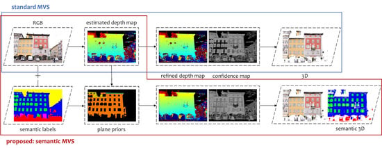
4. Proposed Methodology: Semantic PatchMatch MVS

The proposed semantic PatchMatch MVS approach links the input images with their semantic equivalent using a direct pixel to pixel mapping (Figure 1). Based on [9], it extends the initial idea of [18] by imposing class-specific geometric constraints during the depth map computation step. These geometric constraints are used to optimize the matching cost computation and support thus the depth estimation in textureless areas, but at the same time preserve the details and do not over-smooth. Indeed, semantic labels generally imply geometric constraints, as for pixels belonging to the same class the hypothesis is made that they potentially share also common geometric properties. Other works assume local planarity in the form of triangles [24] or superpixels [22], yet we explicitly link the semantic info to derive geometric constraints by assuming planarity for larger, dominant planar areas of the scene. For instance, in urban scene scenarios, semantically segmented images can provide structure hypothesis as for building facades. Planar walls are assumed to be more likely textureless areas, commonly made of flat surfaces of the same color. However, the method is extendable to other shape priors as well. As image segmentation per se is not the main scope of this work, we used a priori generated labels as in [18,77].

As in the PatchMatch MVS implementation explained in Section 3, stereo pair selection is followed by the depth computation step, where the main core of PatchMatch algorithms takes place. Initial depth values are estimated using the sparse cloud and are further refined using spatial propagation. This iterative procedure will probably converge to a good depth estimate, especially for high resolution images. However, in weakly supported, textureless regions, the photometric score will be dominated by image noise, resulting in wrongly estimated dense points. An overview of the steps of the proposed method are shown in Figure 2.

4.1. Plane Fitting for Depth Prior Generation

The standard PatchMatch iterations output estimated depth values and assigned normal vectors that are to be further refined in the next steps. We use these pixel depth estimates to generate depth and normal priors for every dominant plane present in the scene. In this study, we adopt planar surfaces as they are commonly encountered in urban scenarios, close-range or aerial. PatchMatch depth maps of each view are first projected in the 3D space using the camera projection matrix. Instead of projecting all scene pixels, we use semantic prior masks to project only the subset of points under specific semantic labels that are more likely to include planes (i.e., “wall”, “floor”) (Figure 3b,c). Using the eigenvalues ${\lambda }_1,{\lambda }_2,{\lambda }_3$, 3D points are classified according to their planarity:

$$\frac{{\lambda }_2-{\lambda }_3}{{\lambda }_1},$$

(3)

the points with low planarity values ($p<0.3$) are filtered out. By doing so, isolated groups of points are to be excluded from our further process, since they most probably would not belong to representative dominant planes of the scene but they would rather be outliers. Subsequently, 3D planes in every view are detected using the Efficient RANSAC algorithm [78] as enfolded in CGAL library [79]. RANSAC parameters, $ϵ$ and $cluster$ thresholds, as well as minimun number of points to fit a plane, are adjusted accordingly based on the average spacing of every point cloud so that only significantly large planes are considered valid and avoid, thus, oversegmentation (Figure 3d).

For every detected plane the weighted centroid $C(X,Y,Z)$ and the normal n is calculated. We define the boundaries of each plane in 3D using the minimum bounding rectangle (extent) of each set belonging to the same RANSAC plane. Finally we assign each image pixel that passes the semantic label check to the correct plane using raytracing. For assigning a pixel to its corresponding plane, the pixel has to be inside its extent (projected back to the image) and the plane has to be the closest to the point. Eventually, planar priors are generated only for the semantic classes that we consider locally planar e.g., facade walls. Both depth and normal priors are stored for every image pixel of these regions. These priors are further used to assist the cost computation (Figure 3e).

4.2. Proposed Cost Function

PatchMatch highly relies on the photometric consistency measure (NCC) to correctly select which value from the random estimates is the best depth hypothesis. Our method starts from the mostly good depth estimates calculated by the first iterations of the standard PatchMatch (commonly set $i=4$) and refines the results using the plane priors. Spatial propagation, a fundamental step in PatchMatch, is the procedure when the photometric cost of the current pixel is compared to its neighboring ones and if the values of the latter are better (i.e., lower) they are assigned to the current pixel. On the contrary, the initial estimate is kept if the costs of the neighbors are less reliable (i.e., higher). The cost is defined:

$$cos{t}_{ph}=1-NCC.$$

(4)

The lower the cost, the higher the photometric consistency metric is, resulting in better depth estimates. Even though this approach produces generally accurate results, in textureless areas it often causes the propagation of wrong depth estimates. One possible solution for this would be to directly substitute the estimated depth values in problematic areas with the plane priors calculated in the previous step. However, this would create unreliable outcomes, forcing planarity and smoothing out details. Instead, we propose to adjust the cost function in order to leverage the plane priors, if previously generated for this area, by introducing two additional metrics. Our first metric is based on the shape priors (inherited from the semantic labels in our case) of the pixels that imply geometric constraints and measures the consistency between PatchMatch estimates and plane priors using shift-invariant Gaussian kernel:

$$C_s=e^{\frac{-D^2}{2{\sigma }_1^2}},$$

(5)

where D is the difference between shape priors generated by RANSAC and PatchMatch estimates and ${\sigma }_1$ is a constant. Given the depth prior $d_{prior}$ and the original PatchMatch estimation $d_{ph}$, we define D as:

$$D=\frac{|d_{prior}-d_{ph}|}{d_{prior}}.$$

(6)

If D is very small (i.e., close to zero), it means that the initial estimate is close enough to the “ideal” prior, i.e., we get a reliable hypothesis and PatchMatch depth value is retained and thus propagated. On the contrary, if the depth difference is large, we assume that we are in a problematic region, PatchMatch likely has propagated a wrong estimate and we trust more the prior value.

The second metric, represents the textureness of the pixel’s neighbourhood by calculating the standard deviation of the intensity (color) values in a $N\times N$ window:

$$s_t=\sqrt{\frac{\sum {(i-\mu )}^2}{N\times N}}.$$

(7)

In the presence of evenly colored, textureless surfaces, standard deviation would have very small values, close to zero. This metric indicates the reliability of the photometric score and is critical for avoiding over-smoothing and preserving details. Textureness metrics were also used in [22] but in a different fashion than our formulation. Our textureness coefficient is defined similarly to the semantic prior coefficient in Equation (5) as:

$$C_t=e^{\frac{-s_t^2}{2{\sigma }_2^2}},$$

(8)

where $s_t^2$ is the variance and ${\sigma }_2$ a constant. We leverage both the semantic coefficient $C_s$ (Equation (5)) and the textureness coefficient $C_t$ (Equation (8)) into the initial photometric cost $cos{t}_{ph}$ (Equation (4)) to get the combined cost:

$$cos{t}_{ph,s}=cos{t}_{ph}(1-C_t)+w(1-C_s)C_t,$$

(9)

where w is a weight factor.

Planar regions for which plane priors are available are very likely to be assigned with high photometric cost values, since most of the matches will be ambiguous and thus unreliable. The standard deviation $s_t$ of the intensity of the pixel neighbourhood will probably be close to zero, since color similarity is maximized. In this way, for the planar regions that have high scores, the new cost function will give priority to the prior estimates. On the contrary, for the regions where the original photometric score is reliably calculated the depth estimates will trust more the photometric score. In such a way, plane priors are alleviated with color similarity and erroneous estimates vanish resulting in more reliable depth maps. In other words, when the surface deviates from the plane but has a significant texture variance, the photometric cost is trusted more. Possible outliers will be filtered out from PatchMatch because of no coherence with the neighborhood and in the worst case scenario it will degenerate to the standard case. Example behaviour of the cost function with respect to D and $s_t^2$ variations are shown in Figure 4.

The cost function affects directly not only the depth maps, but also the normal and confidence ones (Figure 2). Noisy regions of the normal maps are also smoothed and information gaps are filled in, since estimated normals are leveraged with the normal prior information. Same holds for confidence maps that reflect the depth estimate reliability of every pixel. In our experiments we show that only two additional PatchMatch iterations with the new cost function were enough to significantly improve the depth and normal map quality, as well as the confidence of every pixel and the final dense 3D point cloud. Indeed, our solution converges relatively fast. Depth maps are further fused adopting the standard approach of [9] as described in Section 3 resulting in a unique dense point cloud.

Following a common dense cloud coloring technique where each fused point in 3D inherits the pixel color of the image from which it is better seen, we use the semantic labels to color the fused dense cloud and generate semantically enriched point clouds. Our semantic PatchMatch approach is built upon the open source library OpenMVS [80], which follows the approach of [9] for the the dense reconstruction.

5. Experiments and Results

5.1. Datasets

Benchmarks with semantically segmented images for accurate 3D reconstruction using MVS are not currently available up to our knowledge. Our method cannot be directly applied to benchmark 3D reconstruction datasets such as ETH3D [3] or Tanks and Temples [2] as other MVS algorithms do [22,23,66], due to the fact that these MVS datasets lack accompanied labelled data. However, in order to be in-line and comparable with the other state of the art techniques, we used three representative ETH3D datasets for which the GT labels were manually annotated. Along with this, we tested our algorithm on our custom datasets [18,77] and the UDD5 benchmark dataset.

ETH3D: We use sequences from the high-resolution (6048 × 4032) datasets for which ground truth 3D data is available: ETH3D-courtyard (38 images) and ETH3D-terrace (23 images) as typical outdoor scenarios and ETH3D-pipes (13 images) for the indoor one. We performed manual labelling for the building facades in order to extract planar regions, as shown in Figure 3. Class labels are the same used in [18,77] for the ETH3D-courtyard and ETH3D-terrace datasets while for the interior scenario ETH3D-pipes we introduce the semantic labels “wall”, “floor”, “door”, “closet” and “other”. In this specific dataset, planes estimation is performed within the classes “wall”, “floor” and “closet”, whereas for the other two only “wall” is considered. For being comparable with the publicly available results of the other state of the art methods tested on the benchmark, images are resampled to 3200 pixels as in [23]. This is a common practice in order to reduce the computational cost and handle large scale datasets, and although dense cloud density is, as expected, partially affected it is considered to be enough for such datasets. For these datasets we perform qualitative comparisons for depth maps (Figure 5) and confidence maps (Figure 6). The resulting 3D dense clouds are evaluated qualitatively (Figure 7) and quantitatively (

Table 1. Accuracy, completeness and $F_1$ score comparisons for tolerance $\tau$ = 2 cm and $\tau$ = 10 cm for the ETH3D benchmark datasets. Values for the other methods are taken from the ETH3D evaluation site. Best values in bold.

		$\mathbf{\tau }$ = 2 cm			$\mathbf{\tau }$ = 10 cm
	Method	Accuracy	Completeness	${\mathit{F}}_{\mathbf{1}}$	Accuracy	Completeness	${\mathit{F}}_{\mathbf{1}}$
ETH3D-terrace	COLMAP	96.79	75.67	84.94	99.29	93.83	96.48
	TAPA-MVS	94.00	82.37	87.80	98.45	98.15	98.30
	ACMM	96.19	84.13	89.76	99.13	96.16	97.62
	ACMP	96.14	84.45	89.92	99.14	96.42	97.76
	PCF-MVS	92.72	84.75	88.56	98.09	97.46	97.78
	OpenMVS	88.72	87.52	88.12	98.00	98.53	98.27
	ours	89.81	88.83	89.32	98.28	98.98	98.63
	ours-no labels	89.77	88.65	89.21	98.26	98.94	98.60
ETH3D-courtyard	COLMAP	88.98	73.47	80.49	99.14	92.20	95.54
	TAPA-MVS	84.69	77.04	80.68	97.64	96.14	96.89
	ACMM	91.35	82.85	86.89	99.51	91.90	95.56
	ACMP	90.83	80.96	85.61	99.43	90.80	94.92
	PCF-MVS	86.12	83.67	84.88	98.43	94.44	96.39
	OpenMVS	80.46	90.10	85.01	97.85	97.63	97.74
	ours	79.66	90.58	84.77	97.61	97.22	97.41
	ours-no labels	79.69	90.43	84.72	97.60	97.04	97.32
ETH3D-pipes	COLMAP	97.77	34.24	50.72	99.18	62.75	76.86
	TAPA-MVS	93.71	63.80	75.91	97.90	86.70	91.96
	ACMM	96.63	53.97	69.26	98.89	66.25	79.34
	ACMP	97.65	53.54	69.16	99.20	65.80	79.12
	PCF-MVS	90.40	69.18	78.38	98.48	88.47	93.21
	OpenMVS	82.33	64.55	72.36	95.95	85.42	90.38
	ours	85.33	73.50	78.97	96.89	93.63	95.23
	ours-no labels	84.19	69.88	76.37	97.32	91.08	94.10

). Results derived with the proposed method are compared against the baseline OpenMVS [80], as well as COLMAP [10] and four recent methods that use geometric prior-assisted PatchMatch: TAPA-MVS [20], ACMM [23], ACMP [24] and PCF-MVS [66].

Custom datasets: Two more scenarios are used in our evaluation, namely PiazzaDuomo (12 high resolution images, 6048 × 4032 px) and PiazzaNavona (5 high resolution images, 4000 × 3000 px). Again, images are resampled to 3200 pixels. Ground truth semantic labels are available from our previous work [77] for the classes “wall”, “window”, “door”, “other”, where “wall” is considered a class in which we search for planar areas. For the dataset PiazzaDuomo, a ground truth 3D point cloud from terrestrial laser scanning is also available. In this scenario, we compare our results with COLMAP [10], TAPA-MVS [20], ACMM [23] and ACMP [24] (

Table 2. Accuracy, completeness and $F_1$ score comparisons of the PiazzaDuomo dataset for $\tau$ = 10 cm.

	Method	Acc.	Compl.	${\mathit{F}}_{\mathbf{1}}$
PiazzaDuomo	COLMAP	88.89	38.00	52.24
	TAPA-MVS	25.56	23.74	24.62
	ACMM	50.87	50.51	50.69
	ACMP	40.92	25.93	31.75
	OpenMVS	70.53	68.55	69.52
	ours	71.08	69.38	70.22

, Figure 8). Qualitative comparison for the dense and confidence maps is also presented (Figure 9).

UDD5:UrbanDrone Dataset UDD5 [45] is a large scale benchmark dataset for segmentation of aerial urban scenarios. We use the training data for which the images labels are given as ground truth (200 images, 4000 × 3000 pixels). UDD5 labels are defined as “vegetation”, “building”, “vehicle”, “road” and “other”. Plane priors are estimated for the class “building” (which includes roofs and facades). Since 3D ground truth data are not available for this dataset, we use it only for qualitative evaluation (Figure 9). For computational efficiency, depth maps are generated in $1/4$ of the original resolution, i.e., 2000 × 1500 pixels.

5.2. Parameter Settings

We ran our tests on an AMD Ryzen 2950X CPU and a GeForce GTX 1070Ti GPU. For a fair comparison with the baseline PatchMatch MVS approach [9] of OpenMVS [80], we keep the same parameter configuration and change only the cost computation for including the class-specific priors. The combined score is computed using $w=0.1$, $N=7$, ${\sigma }_1=0.05$ and ${\sigma }_2=0.03$ that experimentally were proven to be the best trade off values. The depth map filtering step is skipped for the reconstruction of this experimental setup and it is substituted with point cloud filtering, following the OpenMVS parameter settings for the published results available in the ETH3D website. Depth map fusion is then used as enfolded in OpenMVS library [80].

5.3. Evaluation Metrics

According to [2,3], completeness (or recall) r is calculated as the amount of ground truth points for which the distance to the MVS reconstructed points are below a certain threshold. On the contrary, accuracy (or precision) p refers to the ratio of reconstructed points which are within the threshold distance from the ground truth points, without taking into consideration the GT information gaps. Both accuracy and completeness are considered important, and $F1$ score is the harmonic mean of the above measures, defined as $F_1=2(p\times r)/(p+r)$.

6. Discussion

Experimental results on ETH3D sequences and custom datasets show the effectiveness of our approach in handling textureless areas and generating more complete point clouds. Please note that ETH3D-courtyard and ETH3D-terrace are generally complete sequences acquired with dense image networks of high overlap where no particularly problematic textureless areas are present. Indeed, most of the state of the art algorithms achieve good results as shown in Table 1. Even in this case, our approach performs in a competitive way. On the other hand, ETH3D-pipes is one of the most challenging sequences, featuring lower overlap and large textureless areas or reflective surfaces. Our method outperforms the other methods in completeness and $F_1$ score in this particular sequence. Overall, the proposed method generates more complete depth maps (Figure 5) and higher confidence values (Figure 6) for the ETH3D datasets with respect to other MVS methods and the respective point clouds contain less gaps (Figure 7). As shown in Table 1, we achieved better completeness results with respect to all other methods in all three ETH3D datasets for $\tau$ = 2 cm and for $\tau$ = 10 cm except for ETH3D-courtyard in $\tau$ = 10 cm where we rank second. Accuracy and $F_1$ score values are significantly higher than the baseline OpenMVS for ETH3D-pipes, marginally better for ETH3D-terrace, and slightly lower for ETH3D-courtyard for both $\tau$ = 2 cm and $\tau$ = 10 m. However, our $F_1$ score is always among the best ones; other methods that perform well in accuracy (such as COLMAP) suffer in completeness scores since they generate significantly sparser point clouds. The qualitative comparisons of the depth and confidence maps, where available, show that our method delivers more complete depth maps and higher confidence values even in textureless areas where other algorithms fail.

For PiazzaDuomo and PiazzaNavona datasets, the proposed approach generates more complete point clouds with respect to the baseline and other MVS methods. Especially in the low textured regions, we achieve satisfying results in gap filling in the depth maps and higher confidence values (Figure 9, first two rows) while the 3D point clouds lack less information in textureless areas (Figure 8). This is also proven by the completeness score which outperforms all other methods and the second best accuracy after COLMAP (Table 2) that however produces very sparse results (Figure 8a). The PiazzaDuomo and PiazzaNavona datasets have been proven to be challenging, as they feature relatively small overlap with respect to ETH3D datasets and the scenes include many textureless regions (Figure 8). UDD5 dataset is a dense sequence of 200 highly overlapping images. The standard OpenMVS reconstruction was not particularly problematic since the scene was generally well textured. Gaps in depth maps still exist, though they are mainly caused by occlusions. In such cases, our algorithm performs equally well as the standard approach (Figure 9, lower row).

The proposed method relies on the estimation of planar priors in the scene. Typically, regions with erroneous depth estimations result in outliers in 3D and, consequently, the plane fitting procedure is less robust in those regions. Indeed, over some thresholds, RANSAC is not able to cope with these errors, plane priors cannot be accurately calculated and wrong depth estimations will still exist in a similar way as the standard PatchMatch approach of OpenMVS. To validate the effectiveness of our approach in general scenarios where no semantic information is available, we remove the input labels and we search for valid dominant planes across the entire image (ours-no labels). The results show similar performance with our semantic PatchMatch method for the ETH3D-courtyard and ETH3D-terrace sequences with marginally lower accuracy, completeness and $F_{1}score$ values (Table 1). For the ETH3D-pipes sequence, more evident improvement is proven while using the labels (ours), especially in completeness (2–4%) and $F_1$ score (1–2%) with respect to the variant without the labels (ours-no labels) as well as with respect to our baseline OpenMVS. This proves the effectiveness of the semantic PatchMatch approach, as the labels constrain the plane search area performing class-specific assumptions. In this way, it is more likely to fit better planes and propagate correct depth estimates using the priors. Regarding runtime analysis, our method behaves similar to standard OpenMVS, as the two additional iterations add little computational cost to the entire MVS procedure.

As by-product and added value, the proposed method generates also semantically enriched point clouds (Figure 10); each 3D point, beside the real texture information, has also a semantic meaningful attribute inherited from the image annotations.

7. Conclusions

The article introduced a novel approach to leverage plane priors inherited from semantic labels into the MVS process. Based on the standard PatchMatch algorithm implemented in OpenMVS library, we proposed an adapted cost function for improving depth estimations on textureless areas. The method was successfully evaluated on outdoor urban scenes and indoor scenarios available in well-known benchmarks and custom datasets. Although overall metrics do not not always outperform other MVS methods, the presented visual and quantitative results show that depth maps and point clouds are more complete with the proposed method. Lastly, our method also generates semantically enriched dense clouds by projecting the image labels to the 3D points. The additional semantic information used to support depth estimation could be a limitation in the generalization of the proposed method, yet semantically segmented images are increasingly becoming available due to the broad use of deep learning methods. Our code and labelled datasets are to be publicly available.

References

1. Seitz, S.M.; Curless, B.; Diebel, J.; Scharstein, D.; Szeliski, R. A comparison and evaluation of multi-view stereo reconstruction algorithms. In Proceedings of the 2006 IEEE Computer Society Conference on Computer Vision and Pattern Recognition (CVPR’06), New York, NY, USA, 17–22 June 2006; Volume 1, pp. 519–528. [Google Scholar]
2. Knapitsch, A.; Park, J.; Zhou, Q.Y.; Koltun, V. Tanks and temples: Benchmarking large-scale scene reconstruction. ACM Trans. Graph. (ToG) 2017, 36, 1–13. [Google Scholar] [CrossRef]
3. Schops, T.; Schonberger, J.L.; Galliani, S.; Sattler, T.; Schindler, K.; Pollefeys, M.; Geiger, A. A multi-view stereo benchmark with high-resolution images and multi-camera videos. In Proceedings of the IEEE Conference on Computer Vision and Pattern Recognition, Honolulu, HI, USA, 21–26 July 2017; pp. 3260–3269. [Google Scholar]
4. Hirschmuller, H. Stereo processing by semiglobal matching and mutual information. IEEE Trans. Pattern Anal. Mach. Intell. 2007, 30, 328–341. [Google Scholar] [CrossRef]
5. Yao, Y.; Luo, Z.; Li, S.; Fang, T.; Quan, L. Mvsnet: Depth inference for unstructured multi-view stereo. In Proceedings of the European Conference on Computer Vision (ECCV), Munich, Germany, 8–14 September 2018; pp. 767–783. [Google Scholar]
6. Huang, P.H.; Matzen, K.; Kopf, J.; Ahuja, N.; Huang, J.B. Deepmvs: Learning multi-view stereopsis. In Proceedings of the IEEE Conference on Computer Vision and Pattern Recognition, Salt Lake City, UT, USA, 18–23 June 2018; pp. 2821–2830. [Google Scholar]
7. Wang, C.; Miguel Buenaposada, J.; Zhu, R.; Lucey, S. Learning depth from monocular videos using direct methods. In Proceedings of the IEEE Conference on Computer Vision and Pattern Recognition, Salt Lake City, UT, USA, 18–23 June 2018; pp. 2022–2030. [Google Scholar]
8. Bleyer, M.; Rhemann, C.; Rother, C. PatchMatch Stereo-Stereo Matching with Slanted Support Windows. In Proceedings of the British Machine Vision Conference, Dundee, UK, 29 August–2 September 2011; Volume 11, pp. 1–11. [Google Scholar]
9. Shen, S. Accurate multiple view 3d reconstruction using patch-based stereo for large-scale scenes. IEEE Trans. Image Process. 2013, 22, 1901–1914. [Google Scholar] [CrossRef]
10. Schönberger, J.L.; Zheng, E.; Frahm, J.M.; Pollefeys, M. Pixelwise view selection for unstructured multi-view stereo. In Proceedings of the European Conference on Computer Vision, Amsterdam, The Netherlands, 14–16 October 2016; pp. 501–518. [Google Scholar]
11. Zheng, E.; Dunn, E.; Jojic, V.; Frahm, J.M. Patchmatch based joint view selection and depthmap estimation. In Proceedings of the IEEE Conference on Computer Vision and Pattern Recognition, Columbus, OH, USA, 23–24 June 2014; pp. 1510–1517. [Google Scholar]
12. Galliani, S.; Lasinger, K.; Schindler, K. Massively parallel multiview stereopsis by surface normal diffusion. In Proceedings of the IEEE International Conference on Computer Vision, Santiago, Chile, 7–13 June 2015; pp. 873–881. [Google Scholar]
13. Jancosek, M.; Pajdla, T. Exploiting visibility information in surface reconstruction to preserve weakly supported surfaces. Int. Sch. Res. Not. 2014, 2014, 798595. [Google Scholar] [CrossRef]
14. Chen, L.C.; Papandreou, G.; Kokkinos, I.; Murphy, K.; Yuille, A.L. Deeplab: Semantic image segmentation with deep convolutional nets, atrous convolution, and fully connected crfs. IEEE Trans. Pattern Anal. Mach. Intell. 2017, 40, 834–848. [Google Scholar] [CrossRef]
15. Badrinarayanan, V.; Kendall, A.; Cipolla, R. Segnet: A deep convolutional encoder-decoder architecture for image segmentation. IEEE Trans. Pattern Anal. Mach. Intell. 2017, 39, 2481–2495. [Google Scholar] [CrossRef] [PubMed]
16. Paszke, A.; Chaurasia, A.; Kim, S.; Culurciello, E. Enet: A deep neural network architecture for real-time semantic segmentation. arXiv 2016, arXiv:1606.02147. [Google Scholar]
17. Knyaz, V.A.; Kniaz, V.V.; Remondino, F.; Zheltov, S.Y.; Gruen, A. 3D Reconstruction of a Complex Grid Structure Combining UAS Images and Deep Learning. Remote. Sens. 2020, 12, 3128. [Google Scholar] [CrossRef]
18. Stathopoulou, E.K.; Remondino, F. Multi-view stereo with semantic priors. Int. Arch. Photogramm. Remote. Sens. Spat. Inf. Sci. 2019, XLII-2/W15, 1135–1140. [Google Scholar] [CrossRef] [Green Version]
19. Häne, C.; Zach, C.; Cohen, A.; Angst, R.; Pollefeys, M. Joint 3D scene reconstruction and class segmentation. In Proceedings of the IEEE Conference on Computer Vision and Pattern Recognition, Portland, OR, USA, 23–28 June 2013; pp. 97–104. [Google Scholar]
20. Romanoni, A.; Ciccone, M.; Visin, F.; Matteucci, M. Multi-view stereo with single-view semantic mesh refinement. In Proceedings of the IEEE International Conference on Computer Vision Workshops, Venice, Italy, 22–29 October 2017; pp. 706–715. [Google Scholar]
21. Blaha, M.; Rothermel, M.; Oswald, M.R.; Sattler, T.; Richard, A.; Wegner, J.D.; Pollefeys, M.; Schindler, K. Semantically informed multiview surface refinement. In Proceedings of the IEEE International Conference on Computer Vision, Venice, Italy, 22–29 October 2017; pp. 3819–3827. [Google Scholar]
22. Romanoni, A.; Matteucci, M. Tapa-mvs: Textureless-aware patchmatch multi-view stereo. In Proceedings of the IEEE International Conference on Computer Vision, Seoul, Korea, 27 October–2 November 2019; pp. 10413–10422. [Google Scholar]
23. Xu, Q.; Tao, W. Multi-scale geometric consistency guided multi-view stereo. In Proceedings of the IEEE Conference on Computer Vision and Pattern Recognition, Seoul, Korea, 27 October–2 November 2019; pp. 5483–5492. [Google Scholar]
24. Xu, Q.; Tao, W. Planar Prior Assisted PatchMatch Multi-View Stereo. arXiv 2019, arXiv:1912.11744. [Google Scholar]
25. Shotton, J.; Winn, J.; Rother, C.; Criminisi, A. Textonboost for image understanding: Multi-class object recognition and segmentation by jointly modeling texture, layout, and context. Int. J. Comput. Vis. 2009, 81, 2–23. [Google Scholar] [CrossRef] [Green Version]
26. Shotton, J.; Johnson, M.; Cipolla, R. Semantic texton forests for image categorization and segmentation. In Proceedings of the 2008 IEEE conference on computer vision and pattern recognition, Anchorage, AK, USA, 23–28 June 2008; pp. 1–8. [Google Scholar]
27. Fulkerson, B.; Vedaldi, A.; Soatto, S. Class segmentation and object localization with superpixel neighborhoods. In Proceedings of the 2009 IEEE 12th International Conference on Computer Vision, Kyoto, Japan, 4 October–29 September 2009; pp. 670–677. [Google Scholar]
28. LeCun, Y.; Bengio, Y.; Hinton, G. Deep learning. Nature 2015, 521, 436–444. [Google Scholar] [CrossRef]
29. Krizhevsky, A.; Sutskever, I.; Hinton, G.E. Imagenet classification with deep convolutional neural networks. Adv. Neural Inf. Process. Syst. 2012, 25, 1097–1105. [Google Scholar] [CrossRef]
30. Simonyan, K.; Zisserman, A. Very deep convolutional networks for large-scale image recognition. arXiv 2014, arXiv:1409.1556. [Google Scholar]
31. He, K.; Gkioxari, G.; Dollár, P.; Girshick, R. Mask r-cnn. In Proceedings of the IEEE International Conference on Computer Vision, Venice, Italy, 22–29 October 2017; pp. 2961–2969. [Google Scholar]
32. Szegedy, C.; Liu, W.; Jia, Y.; Sermanet, P.; Reed, S.; Anguelov, D.; Erhan, D.; Vanhoucke, V.; Rabinovich, A. Going deeper with convolutions. In Proceedings of the IEEE Conference on Computer Vision and Pattern Recognition, Boston, MA, USA, 7–12 June 2015; pp. 1–9. [Google Scholar]
33. Szegedy, C.; Vanhoucke, V.; Ioffe, S.; Shlens, J.; Wojna, Z. Rethinking the inception architecture for computer vision. In Proceedings of the IEEE Conference on Computer Vision and Pattern Recognition, Las Vegas, NV, USA, 27–30 June 2016; pp. 2818–2826. [Google Scholar]
34. Szegedy, C.; Ioffe, S.; Vanhoucke, V.; Alemi, A. Inception-v4, inception-resnet and the impact of residual connections on learning. In Proceedings of the AAAI Conference on Artificial Intelligence, Francisco, CA, USA, 4–9 February 2017; Volume 31. [Google Scholar]
35. Huang, G.; Liu, Z.; Van Der Maaten, L.; Weinberger, K.Q. Densely connected convolutional networks. In Proceedings of the IEEE Conference on Computer Vision and Pattern Recognition, Honolulu, HI, USA, 21–26 July 2017; pp. 4700–4708. [Google Scholar]
36. Long, J.; Shelhamer, E.; Darrell, T. Fully convolutional networks for semantic segmentation. In Proceedings of the IEEE Conference on Computer Vision and Pattern Recognition, Boston, MA, USA, 7–12 June 2015; pp. 3431–3440. [Google Scholar]
37. Minaee, S.; Boykov, Y.; Porikli, F.; Plaza, A.; Kehtarnavaz, N.; Terzopoulos, D. Image segmentation using deep learning: A survey. arXiv 2020, arXiv:2001.05566. [Google Scholar]
38. Brostow, G.J.; Fauqueur, J.; Cipolla, R. Semantic object classes in video: A high-definition ground truth database. Pattern Recognit. Lett. 2009, 30, 88–97. [Google Scholar] [CrossRef]
39. Riemenschneider, H.; Bódis-Szomorú, A.; Weissenberg, J.; Van Gool, L. Learning where to classify in multi-view semantic segmentation. In Proceedings of the European Conference on Computer Vision, Zurich, Switzerland, 6–12 September 2014; pp. 516–532. [Google Scholar]
40. Cordts, M.; Omran, M.; Ramos, S.; Rehfeld, T.; Enzweiler, M.; Benenson, R.; Franke, U.; Roth, S.; Schiele, B. The cityscapes dataset for semantic urban scene understanding. In Proceedings of the IEEE Conference on Computer Vision and Pattern Recognition, Las Vegas, NV, USA, 27–30 June 2016; pp. 3213–3223. [Google Scholar]
41. Armeni, I.; Sax, S.; Zamir, A.R.; Savarese, S. Joint 2d-3d-semantic data for indoor scene understanding. arXiv 2017, arXiv:1702.01105. [Google Scholar]
42. Song, S.; Lichtenberg, S.P.; Xiao, J. Sun rgb-d: A rgb-d scene understanding benchmark suite. In Proceedings of the IEEE Conference on Computer Vision and Pattern Recognition, Boston, MA, USA, 7–12 June 2015; pp. 567–576. [Google Scholar]
43. Silberman, N.; Hoiem, D.; Kohli, P.; Fergus, R. Indoor segmentation and support inference from rgbd images. In Proceedings of the European Conference on Computer Vision, Florence, Italy, 7–13 October 2012; pp. 746–760. [Google Scholar]
44. McCormac, J.; Handa, A.; Leutenegger, S.; Davison, A.J. Scenenet rgb-d: 5m photorealistic images of synthetic indoor trajectories with ground truth. arXiv 2016, arXiv:1612.05079. [Google Scholar]
45. Chen, Y.; Wang, Y.; Lu, P.; Chen, Y.; Wang, G. Large-scale structure from motion with semantic constraints of aerial images. In Proceedings of the Chinese Conference on Pattern Recognition and Computer Vision (PRCV), Guangzhou, China, 23–26 November 2018; pp. 347–359. [Google Scholar]
46. Lyu, Y.; Vosselman, G.; Xia, G.S.; Yilmaz, A.; Yang, M.Y. UAVid: A semantic segmentation dataset for UAV imagery. ISPRS J. Photogramm. Remote. Sens. 2020, 165, 108–119. [Google Scholar] [CrossRef]
47. Rottensteiner, F.; Sohn, G.; Jung, J.; Gerke, M.; Baillard, C.; Benitez, S.; Breitkopf, U. The ISPRS benchmark on urban object classification and 3D building reconstruction. Ann. Photogramm. Remote. Sens. Spat. Inf. Sci. I-3 2012, 1, 293–298. [Google Scholar] [CrossRef] [Green Version]
48. Ladickỳ, L.; Sturgess, P.; Russell, C.; Sengupta, S.; Bastanlar, Y.; Clocksin, W.; Torr, P.H. Joint optimization for object class segmentation and dense stereo reconstruction. Int. J. Comput. Vis. 2012, 100, 122–133. [Google Scholar] [CrossRef] [Green Version]
49. Schneider, L.; Cordts, M.; Rehfeld, T.; Pfeiffer, D.; Enzweiler, M.; Franke, U.; Pollefeys, M.; Roth, S. Semantic stixels: Depth is not enough. In Proceedings of the 2016 IEEE Intelligent Vehicles Symposium (IV), Gotenburg, Sweden, 19–22 June 2016; pp. 110–117. [Google Scholar]
50. Kundu, A.; Li, Y.; Dellaert, F.; Li, F.; Rehg, J.M. Joint semantic segmentation and 3d reconstruction from monocular video. In Proceedings of the European Conference on Computer Vision, Zurich, Switzerland, 6–12 September 2014; pp. 703–718. [Google Scholar]
51. Zhang, C.; Wang, L.; Yang, R. Semantic segmentation of urban scenes using dense depth maps. In Proceedings of the European Conference on Computer Vision, Crete, Greece, 5–11 September 2010; pp. 708–721. [Google Scholar]
52. Häne, C.; Zach, C.; Cohen, A.; Pollefeys, M. Dense semantic 3d reconstruction. IEEE Trans. Pattern Anal. Mach. Intell. 2016, 39, 1730–1743. [Google Scholar] [CrossRef]
53. Savinov, N.; Häne, C.; Ladicky, L.; Pollefeys, M. Semantic 3d reconstruction with continuous regularization and ray potentials using a visibility consistency constraint. In Proceedings of the IEEE Conference on Computer Vision and Pattern Recognition, Las Vegas, NV, USA, 27–30 June 2016; pp. 5460–5469. [Google Scholar]
54. Blaha, M.; Vogel, C.; Richard, A.; Wegner, J.D.; Pock, T.; Schindler, K. Large-scale semantic 3d reconstruction: An adaptive multi-resolution model for multi-class volumetric labeling. In Proceedings of the IEEE Conference on Computer Vision and Pattern Recognition, Las Vegas, NV, USA, 27–30 June 2016; pp. 3176–3184. [Google Scholar]
55. Cherabier, I.; Schonberger, J.L.; Oswald, M.R.; Pollefeys, M.; Geiger, A. Learning priors for semantic 3d reconstruction. In Proceedings of the European Conference on Computer Vision (ECCV), Munich, Germany, 8–14 September 2018; pp. 314–330. [Google Scholar]
56. Yingze Bao, S.; Chandraker, M.; Lin, Y.; Savarese, S. Dense object reconstruction with semantic priors. In Proceedings of the IEEE Conference on Computer Vision and Pattern Recognition, Portland, OR, USA, 23–28 June 2013; pp. 1264–1271. [Google Scholar]
57. Ulusoy, A.O.; Black, M.J.; Geiger, A. Semantic multi-view stereo: Jointly estimating objects and voxels. In Proceedings of the 2017 IEEE Conference on Computer Vision and Pattern Recognition (CVPR), Portland, OR, USA, 23–28 June 2017; pp. 4531–4540. [Google Scholar]
58. Furukawa, Y.; Curless, B.; Seitz, S.M.; Szeliski, R. Manhattan-world stereo. In Proceedings of the 2009 IEEE Conference on Computer Vision and Pattern Recognition, Miami, FL, USA, 20–25 June 2009; pp. 1422–1429. [Google Scholar]
59. Gallup, D.; Frahm, J.M.; Pollefeys, M. Piecewise planar and non-planar stereo for urban scene reconstruction. In Proceedings of the 2010 IEEE Computer Society Conference on Computer Vision and Pattern Recognition, San Francisco, CA, USA, 13–18 June 2010; pp. 1418–1425. [Google Scholar]
60. Chen, W.; Hou, J.; Zhang, M.; Xiong, Z.; Gao, H. Semantic stereo: Integrating piecewise planar stereo with segmentation and classification. In Proceedings of the 2014 4th IEEE International Conference on Information Science and Technology, Shenzhen, China, 26–28 April 2014; pp. 200–204. [Google Scholar]
61. Guney, F.; Geiger, A. Displets: Resolving stereo ambiguities using object knowledge. In Proceedings of the IEEE Conference on Computer Vision and Pattern Recognition, Boston, MA, USA, 7–12 June 2015; pp. 4165–4175. [Google Scholar]
62. Barnes, C.; Shechtman, E.; Finkelstein, A.; Goldman, D.B. PatchMatch: A randomized correspondence algorithm for structural image editing. ACM Trans. Graph. 2009, 28, 24. [Google Scholar] [CrossRef]
63. Besse, F.O. PatchMatch Belief Propagation for Correspondence Field Estimation and Its Applications. Ph.D. Thesis, University College London, London, UK, 2013. [Google Scholar]
64. Heise, P.; Klose, S.; Jensen, B.; Knoll, A. Pm-huber: Patchmatch with huber regularization for stereo matching. In Proceedings of the IEEE International Conference on Computer Vision, Sydney, Australia, 1–8 December 2013; pp. 2360–2367. [Google Scholar]
65. Duggal, S.; Wang, S.; Ma, W.C.; Hu, R.; Urtasun, R. Deeppruner: Learning efficient stereo matching via differentiable patchmatch. In Proceedings of the IEEE International Conference on Computer Vision, Seoul, Korea, 27 October–2 November 2019; pp. 4384–4393. [Google Scholar]
66. Kuhn, A.; Lin, S.; Erdler, O. Plane completion and filtering for multi-view stereo reconstruction. In Proceedings of the German Conference on Pattern Recognition, Dortmund, Germany, 10–13 September 2019; pp. 18–32. [Google Scholar]
67. Liu, H.; Tang, X.; Shen, S. Depth-map completion for large indoor scene reconstruction. Pattern Recognit. 2020, 99, 107112. [Google Scholar] [CrossRef]
68. Schonberger, J.L.; Frahm, J.M. Structure-from-motion revisited. In Proceedings of the IEEE Conference on Computer Vision and Pattern Recognition, Las Vegas, NV, USA, 27–30 June 2016; pp. 4104–4113. [Google Scholar]
69. Wang, Y.; Guan, T.; Chen, Z.; Luo, Y.; Luo, K.; Ju, L. Mesh-Guided Multi-View Stereo With Pyramid Architecture. In Proceedings of the IEEE/CVF Conference on Computer Vision and Pattern Recognition, Seattle, WA, USA, 14–19 June 2020; pp. 2039–2048. [Google Scholar]
70. Scharstein, D.; Szeliski, R. A taxonomy and evaluation of dense two-frame stereo correspondence algorithms. Int. J. Comput. Vis. 2002, 47, 7–42. [Google Scholar] [CrossRef]
71. Scharstein, D.; Hirschmüller, H.; Kitajima, Y.; Krathwohl, G.; Nešić, N.; Wang, X.; Westling, P. High-resolution stereo datasets with subpixel-accurate ground truth. In Proceedings of the German Conference on Pattern Recognition, Münster, Germany, 2–5 September 2014; pp. 31–42. [Google Scholar]
72. Strecha, C.; Von Hansen, W.; Van Gool, L.; Fua, P.; Thoennessen, U. On benchmarking camera calibration and multi-view stereo for high resolution imagery. In Proceedings of the 2008 IEEE conference on computer vision and pattern recognition, Anchorage, AK, USA, 23–28 June 2008; pp. 1–8. [Google Scholar]
73. Menze, M.; Geiger, A. Object scene flow for autonomous vehicles. In Proceedings of the IEEE Conference on Computer Vision and Pattern Recognition, Boston, MA, USA, 7–12 June 2015; pp. 3061–3070. [Google Scholar]
74. Geiger, A.; Lenz, P.; Urtasun, R. Are we ready for autonomous driving? The KITTI vision benchmark suite. In Proceedings of the 2012 IEEE Conference on Computer Vision and Pattern Recognition, Providence, RI, USA, 16–21 June 2012; pp. 3354–3361. [Google Scholar]
75. Jensen, R.; Dahl, A.; Vogiatzis, G.; Tola, E.; Aanæs, H. Large scale multi-view stereopsis evaluation. In Proceedings of the 2014 IEEE Conference on Computer Vision and Pattern Recognition, Columbus, OH, USA, 23–28 June 2014; pp. 406–413. [Google Scholar]
76. Aanæs, H.; Jensen, R.R.; Vogiatzis, G.; Tola, E.; Dahl, A.B. Large-Scale Data for Multiple-View Stereopsis. Int. J. Comput. Vis. 2016, 120, 153–168. [Google Scholar] [CrossRef] [Green Version]
77. Stathopoulou, E.K.; Remondino, F. Semantic photogrammetry – boosting image-based 3D reconstruction with semantic labelling. Int. Arch. Photogramm. Remote. Sens. Spat. Inf. Sci. 2019, XLII-2/W9, 685–690. [Google Scholar] [CrossRef] [Green Version]
78. Schnabel, R.; Wahl, R.; Klein, R. Efficient RANSAC for point-cloud shape detection. In Computer Graphics Forum; Wiley Online Library: Hoboken, NJ, USA, 2007; Volume 26, pp. 214–226. [Google Scholar]
79. CGAL (Computational Geometry Algorithms Library). Available online: https://www.cgal.org (accessed on 5 February 2021).
80. Cernea, D. OpenMVS: Multi-View Stereo Reconstruction Library. Available online: https://github.com/cdcseacave/openMVS (accessed on 5 February 2021).
Figure 1. Overview of the proposed method leveraging semantic information into the 3D dense point cloud reconstruction. Per pixel labels are used to generate class specific geometric priors to support depth map computation in problematic textureless areas and produce a more complete point cloud enriched also with the semantic information.
Remotesensing 13 01053 g001
Figure 2. The standard PatchMatch pipeline [9] vs. the proposed method. From left to right: the input image and the respective estimated depth map after standard PatchMatch iterations. In the upper part, the standard approach outputs filtered depth maps (gap interpolation and small segment removal) as well as confidence and normal maps. In the proposed approach (lower part), extra semantic iterations are added after the geometric prior estimation. Resulting depth maps contain less gaps, normal maps are smoother and confidence is higher (scale black to white, with white representing higher confidence).
Remotesensing 13 01053 g002
Figure 3. Plane prior estimation: input image (a); respective labels (b) for semantic classes: sky (yellow), wall (blue), window (green), door (purple), other (red); binary mask for planar classes (c); the estimated normal prior map for the RANSAC planes detected in 3D (d) and their respective depth priors in color scale (e) with blue being the closest and red the farthest.
Remotesensing 13 01053 g003
Figure 4. The combined score c p h , s given a standard photometric score c p h = 0.4 (relatively low confidence) with respect to: (a) the depth difference D for and s t 2 = 0.0001 (textureless area); (b) the s t 2 and D = 0.01 .
Remotesensing 13 01053 g004
Figure 5. Qualitative depth map comparison of our method with other state of the art algorithms for the ETH3D benchmark sequences terrace, courtyard, and pipes. Labels for walls and ceilings have been used in our method to improve the depth estimation. GT depth maps look sparse as they contain empty pixels [3]. All other depth maps are scaled to the GT color scale. (a) RGB image; (b) GT; (c) COLMAP; (d) OpenMVS; (e) proposed.
Remotesensing 13 01053 g005
Figure 6. Qualitative confidence map comparison of our method with respect to the baseline OpenMVS on the ETH3D datasets. Scale black to white, where black means lower confidence. It is evident that the plane priors increase the confidence, especially where textureless areas are present in ETH3D-terrace (ceiling) and ETH3D-pipes (orange panel, closet). For ETH3D-courtyard where the not particularly textureless areas exist, the confidence remains mostly the same. (a) RGB image; (b) OpenMVS; (c) proposed.
Remotesensing 13 01053 g006
Figure 7. Qualitative point cloud comparison of our method with other state of the art algorithms for the ETH3D benchmark sequences terrace, courtyard and pipes. Dense reconstructions for the state of the art methods are as in ETH3D evaluation site. (a) COLMAP; (b) TAPA-MVS; (c) ACMM; (d) ACMP; (e) OpenMVS; (f) ours.
Remotesensing 13 01053 g007
Figure 8. Qualitative point cloud comparison for PiazzaDuomo (first two rows) and PiazzaNavona: state of the art baselines results versus the proposed method (last column). (a) COLMAP; (b) ACMM; (c) ACMP; (d) TAPA-MVS; (e) OpenMVS; (f) proposed.
Remotesensing 13 01053 g008
Figure 9. Qualitative depth and confidence map comparison of our method with respect to the baseline OpenMVS on our custom datasets (PiazzaDuomo and PiazzaNavona) and the UDD5 dataset. The proposed method improves depth estimations and achieve higher confidence scores in problematic planar areas for PiazzaDuomo and PiazzaNavona. In UDD5, where no evident textureless areas exist, it performs like standard OpenMVS. (a) RGB image; (b) OpenMVS-depth; (c) proposed-depth; (d) OpenMVS-conf; (e) proposed-conf.
Remotesensing 13 01053 g009
Figure 10. Dense point clouds generated by our method (left) and their semantically enriched equivalents (right). PiazzaDuomo, PiazzaNavona, ETH-terrace and ETH-courtyard follow the same class labels, namely “wall” (blue), “window” (green), “door” (pink), “other” (red). For the interior dataset ETH-pipes we set “wall” (blue), “floor” (orange), “closet” (grey), “door” (pink) and “other” (red). Aerial dataset UDD5 follows: “vegetation” (green), “building” (purple), “road” (pink), “vehicle” (blue).
Remotesensing 13 01053 g010