Article

Clustering of Rainfall Types Using Micro Rain Radar and Laser Disdrometer Observations in the Tropical Andes

by
Gabriela Urgilés
1,2,
Rolando Célleri
1,2,
Katja Trachte
3,
Jörg Bendix
4 and
Johanna Orellana-Alvear
1,4,*
1
Departamento de Recursos Hídricos y Ciencias Ambientales, Universidad de Cuenca, Cuenca EC010207, Ecuador
2
Facultad de Ingeniería, Universidad de Cuenca, Cuenca EC010207, Ecuador
3
Institute for Environmental Sciences, Brandenburg University of Technology (BTU), Cottbus-Senftenberg, D-03046 Cottbus, Germany
4
Laboratory for Climatology and Remote Sensing, Philipps-University Marburg, D-35032 Marburg, Germany
*
Author to whom correspondence should be addressed.
Remote Sens. 2021, 13(5), 991; https://doi.org/10.3390/rs13050991
Submission received: 28 January 2021 / Revised: 27 February 2021 / Accepted: 1 March 2021 / Published: 5 March 2021
(This article belongs to the Special Issue Remote Sensing of the Water Cycle in Mountain Regions)

Abstract

:
Lack of rainfall information at high temporal resolution in areas with a complex topography as the Tropical Andes is one of the main obstacles to study its rainfall dynamics. Furthermore, rainfall types (e.g., stratiform, convective) are usually defined by using thresholds of some rainfall characteristics such as intensity and velocity. However, these thresholds highly depend on the local climate and the study area. In consequence, these thresholds are a constraining factor for the rainfall class definitions because they cannot be generalized. Thus, this study aims to analyze rainfall-event types by using a data-driven clustering approach based on the k-means algorithm that allows accounting for the similarities of rainfall characteristics of each rainfall type. It was carried out using three years of data retrieved from a vertically pointing Micro Rain Radar (MRR) and a laser disdrometer. The results show two main rainfall types (convective and stratiform) in the area which highly differ in their rainfall features. In addition, a mixed type was found as a subgroup of the stratiform type. The stratiform type was found more frequently throughout the year. Furthermore, rainfall events of short duration (less than 70 min) were prevalent in the study area. This study will contribute to analyze the rainfall formation processes and the vertical profile.

Graphical Abstract

1. Introduction

Precipitation is among the most important components of the hydrologic cycle because it triggers important processes that determine water distribution and availability [1,2,3]. In addition, precipitation is characterized by a high spatiotemporal variability. This is particularly true in the Tropical Andes, where complex topography is a key factor that influences rainfall processes [4]. Here, precipitation variability has been studied only at a certain extent [5,6,7]. This is because of the lack of high temporal resolution data, which is one of the main obstacles to understand the rainfall processes and dynamics in this area [8]. Usually, rainfall characteristics such as rain rate are used to study rainfall variability [6]. Moreover, microphysical characteristics (e.g., drop size distribution) and the study of the vertical profile of the rainfall allow to improve the knowledge about microphysical processes that govern the formation of the hydrometeors and to identify rainfall types. This rainfall variability can be captured by remote sensing observation with Micro Rain Radar (MRR) and laser disdrometers. The advantage of these instruments is that they not only enable to quantify the rainfall but also allow for the analysis of its microphysical attributes [9,10].
MRRs are instruments that measure the characteristics of the precipitation along its vertical profile. MRRs retrieve the reflectivity profile, drop size distribution (DSD), rain rate, velocity, and liquid water content (LWC) [9] for different atmospheric layers. These characteristics allow for the analysis of the vertical structure of the rain. They also allow to differentiate between rain types (convective and stratiform rain) and to identify the height of the Melting Layer (ML) [2,11,12,13]. Besides, disdrometers are instruments that retrieve characteristics as particle spectrum, the rain rate, the quantity, and the type of rain [10]. These instruments have been used to analyze the rainfall dynamic in mountain areas [4,12,14,15,16,17]. In the Tropical Andes, the diurnal dynamics of the precipitation were studied by Bendix et al. [16] using MRR data. The author found that rainfall is mostly of stratiform type and the afternoon events are influenced by local convection. A study in Peru and Bolivia using MRR data [12] showed the dominance of stratiform events during the night, and suggested that the height of ML is an indicator of climate change. Using microphysical data (e.g., mean volume diameter Dm) obtained from laser disdrometers, Orellana-Alvear et al. [4] analyzed rainfall types at three sites with different height in the Andes Cordillera in Ecuador. The authors found that convective type (rainfall associated with higher rain rate and Dm) was more common in the lower elevation sites while light rain was more frequent in higher sites. Seidel et al. [14] using MRR data, found that short events (less than 3 h) were dominant in the Tropical Andes and nocturnal precipitation is more of the stratiform type.
Previous studies highlight the importance of differentiating between rainfall types [3,17,18,19], principally to analyze the rainfall behavior and find patterns in the rainfall attributes. Furthermore, the definition of rainfall types is useful for improving the quantitative precipitation estimation (e.g., Z-R relation) [4]. Usually, rainfall types (e.g., stratiform and convective) are defined by using some rainfall characteristics thresholds such as rain rate [19,20,21]; DSD [22,23] and; reflectivity [24]. Furthermore, in the case of the reflectivity profile, it is used to determine the ML presence, which is also used to determine rainfall types [11,25]. However, these thresholds are site specific [21] and depend mainly on the local climate and the study area. This makes rainfall classification closely related to independent, arguably subjective decisions rather than the possibility of extracting knowledge only from the interactions between rainfall characteristics. This can be overcome using clustering analysis.
This is a machine learning tool that allows grouping objects with similar characteristics only based on the data. Clustering analysis based on the hierarchical and k-means algorithm had been successfully used to classify rainfall events in different studies such as Dilmi et al. [26], dos Santos et al. [27], Fang et al. [28], and Peng and Wang [29]. These studies were carried out in subtropical regions [26,28,29] and tropical semiarid regions [27]. However, there is no report of the application of these techniques in tropical high mountains up to date.
In this context, this study aims to analyze rainfall-event types in the Tropical Andes by using a clustering approach based on the k-means algorithm that allows accounting for the similarities of rainfall characteristics (e.g., duration, rain rate, drop size distribution) of each rainfall type. This will allow for the improvement of the knowledge of rainfall dynamics and its occurrence in the region.

2. Study Site and Data

2.1. Study Site

The study area Balzay (2°53′S, 79°02′W) is located at 2610 m above sea level (a.s.l), in the outskirts of the city of Cuenca in the Tropical Andes of southern Ecuador, as shown in Figure 1. Balzay is located in the inter-Andean depression [30] and shows a bimodal rainfall regime with two wet seasons in the months March-April-May and October. The mean annual precipitation is 969 mm [4] and the mean temperature is 14 °C [31]. The precipitation is mainly driven by the displacement of the Intertropical Convergence Zone (ITCZ) [32,33]. The ITCZ is defined as the zone in the vicinity of the equator, where the trade winds from the north and south converge [34]. The climate in Ecuador shows high variability in part due to the presence of the Andes Cordillera. In the inter-Andean depression, due to the impact of the ITCZ, the tropical Amazon air masses from the East and the Pacific coastal regimen from the West are the main factors that control the climatology of the area [35].

2.2. Instruments

The instruments used in this study are the Micro Rain Radar (MRR) [9] and the laser disdrometer (Thies Clima LPM—Laser Precipitation Monitor) [10]. A detailed explanation of the instruments’ operation is provided in the following sections.

2.2.1. Micro Rain Radar

The MRR is a vertically pointing frequency modulated continuous wave (FM-CW) doppler radar. It operates at 24.1 GHz and 12.5 mm wavelength. The radar transmits a signal along a vertical orientation in the atmosphere over the antenna [9,36].
The primary advantage of the MRR is its high sensitivity and temporal resolution to detect small amounts of precipitation (i.e., low rain rates) [9]. The MRR detects droplets with diameters between 0.25 to 6 mm [37], and it assumes water drops are spherical. The MRR retrieves basically the Doppler spectra of the falling droplets and radar reflectivity where parameters like the mean fall velocity, droplet concentration, rain liquid water content, and rain rate are derived from. The details of the parameters derivation can be found in [9,36,37,38]. The MRR records these parameters for all the vertical profile.
The vertical profile consists of 31 height steps (gates) whose maximum and minimum height resolution is defined by the user and range between 10 and 1000 m. In our case, the MRR was operated with a height resolution of 100 m and the data were captured with a 1-min frequency.

2.2.2. Disdrometer

The disdrometer used in this study is a Thies Clima Laser precipitation monitor (LPM) [10], which is based on a laser sensor that produces a horizontal light beam. This sensor has a wavelength of 785 nm and the measuring area is 45.6 cm2. When a precipitation particle falls through the light beam, the receiving signal is attenuated. The particle diameter is estimated from the reduction in the signal amplitude while its fall velocity is calculated from the duration of the decreased signal. Each drop is assigned to one of 22 size bins and to one of 20 velocity bins. The size bins are between 0.125 and 8 mm and the velocity bins are between 0 and 10 m s−1. Later, a telegram is sent every minute. This shows the number of drops that the LPM detected in each class depending on the bin combination (diameter-velocity). The LPM retrieves the particle spectrum, the rain rate, the quantity, and the type of precipitation. Data were captured with 5-min frequency, as a result of averaging 1-min observations.

2.3. Data Availability and Quality Control

Three years of data, from February 2017 to February 2020 of both instruments were used in this study. The performance of the disdrometer data has been evaluated in [39,40]. In spite of the good performance of the disdrometer, it shows some issues at high wind speeds (>15 m s−1) [41], which, however, were not present in our disdrometer records [4]. Furthermore, to eliminate uncertainty measurements obtained from misclassification of particles, margin fallers and splashing effect, we employed the methodology used in Orellana-Alvear et al. [4]. Details regarding the quality control method can be found in Orellana-Alvear et al. [4] and Friedrich et al. [41]. In the case of the MRR, the data were averaged to 5-min. Several parameters of the MRR such as rain rate (mm h−1), mean fall velocity (m s−1), liquid water content (g m−3), droplet concentration (m−3 mm−1), and radar reflectivity (dBZ) were used for the rainfall classification process.
The validity of the MRR data has been reported by many researchers [11,19,40,42,43]. These studies showed a good agreement between MRR and different types of disdrometer (OTT Parsivel, Joss-Waldvogel and LPM) through a correlation analysis. Thus, to ensure the validity of the MRR measurements, we compared the rain rate observed by the MRR at the lowest height (100m) with the rain rate obtained from the collocated disdrometer at 30-min cumulative interval (Figure 2). This comparison was performed by using the determination coefficient (R2). The coefficient of determination between MRR and LPM rain rate data was 0.74 (Figure 2). Therefore, we had a good fit in spite of the difference in height where each sensor is monitoring the rainfall (i.e., the disdrometer is located at ground level while the MRR first range of monitoring is 0–100 m).
As shown in Figure 2, the MRR tended to slightly underestimate the rainfall amount compared to disdrometer observations. Nevertheless, the MRR showed some outliers especially in higher values. Figure 2 also suggests that the MRR tend to overestimate the rainfall above 10 mm 30 min−1. Sarkar et al. [40] found that the LPM and MRR had a good fit (R2 = 0.74). The author suggested that over 60 mm h−1, the MRR has a high probability of underestimating the measures of rain rate. In addition, Rollenbeck et al. [44] compared the precipitation measurements between five recording devices. The author found that the MRR underestimate the precipitation. The MRR had a high sensitivity to detect light rain, but it had problems detecting higher rain rates [44,45]. These studies agree with our results and show the good fit between both instruments. Thus, we derived the drop size distribution (m−3 mm−1) from the disdrometer data. It was calculated from the number of drops for each size and velocity bins [10]. The details of the drop spectrum calculation can be found in [4,40,46].

3. Methods

First, we selected rainfall events from the available time series by using three criteria which are detailed in Section 3.1. Then, for each of them, we determined individual rainfall event characteristics (e.g., duration, maximum rain rate, etc.) derived from the MRR and LPM data. Finally, we applied the k-means algorithm that clusters these events based on their derived characteristics. A detailed explanation of the last steps is provided in Section 3.2.

3.1. Rainfall Events Selection

Representative data of the study period were obtained through the delineation of rainfall events using three criteria: (i) minimum interevent time, (ii) minimum total rainfall accumulation, and (iii) minimum duration. The minimum interevent time is defined as the minimum lapse of time for a dry period (i.e., no rainfall occurrence or less than a threshold) between rainfall events, which is necessary to classify two events as independent. In this study, we used the threshold of rain rate greater than 0.05 mm min−1 for each time step. This threshold was identified using a sensitivity analysis by testing different values between 0.01 and 0.1 mm min−1. The value of 0.05 mm min−1 was selected because it eliminated the long tails and discontinuities that lower rain rate values showed in the events. The minimum total rainfall accumulation refers to the rainfall total during the event. The minimum duration is the time where the rainfall was continuous (without gaps) [47,48]. To identify the proper thresholds for these values we performed a sensitivity analysis which was carried out by using a variation between a range of values of each criterion (minimum interevent time, minimum total rainfall accumulation, and minimum duration) with the purpose of getting a probability distribution. This distribution was used to find a threshold where the number of events got steady for each criterion and thus, we got a trade-off between the number of events and their representativeness. The range of values to find the proper threshold were: (i) 20–60 min for minimum interevent time; (ii) 2–8 mm for minimum total rainfall accumulation per event and; (iii) 10–30 min for minimum duration. The methodology of Orellana-Alvear et al. [4] was used as a starting point to determine such thresholds. Finally, rainfall events that met the criteria were selected for the current study.

3.2. Rainfall Classification

3.2.1. Derivation of Rainfall Events Characteristics

Rainfall event characteristics are used to describe and synthesize the behavior of a rainfall event [26]. After the rainfall events were selected, several of their temporal (e.g., duration) and hydrometeorological (e.g., rainfall accumulation) characteristics were picked out for the rainfall classification process. However, there is no universally agreed set of characteristics to describe a rainfall event [26]. Generally, choosing the rainfall characteristics depends on the instrument, its measured variables, and the objective of the study. Here, we used the characteristics obtained from the MRR and the LPM; these include hydrological and microphysical information of the rainfall events (Table A1).

Derivation of MRR and Disdrometer Characteristics

We used four hydrological characteristics of rainfall events of the lower height bin of the MRR, namely rain rate (mm h−1), mean fall velocity (m s−1), liquid water content (g m−3), and radar reflectivity (dBZ). Moreover, rainfall accumulation and the duration of the event were calculated.
Regarding microphysical data, the LPM retrieved the drop spectra N(D) (m−3 mm−1) and drop diameters D (mm). These characteristics are used to represent the Drop Size Distribution (DSD) [49] at each time step. Nonetheless, we needed to combine these characteristics to get a representative DSD for each rainfall event. So, we derived the mean volume diameter (Dm) in mm that represents the proportion between the fourth and third moment of the DSD, as defined by [50]. It is frequently used to represent the DSD of a rainfall event [4,26,43,51,52]. Finally, we analyzed the characteristic distribution and extracted the mean, maximum, minimum, and median value for characterizing the rainfall properties within each event.

Determination of the Melting Layer

The Melting Layer (ML) is an important characteristic, commonly used to identify rainfall classes [11,25,53]. The ML determination is based on the identification of a Bright Band (BB) signature in the vertical profile of the reflectivity. This BB detection consists in determining the prominent increase of the values in the reflectivity profile at specific gates, using the maximum slope found in the reflectivity profile [11,54,55]. This band is a combination of water, air, and ice that highly increase the reflectivity values at certain gates of the vertical profile. In addition, another factor that influences the increase in reflectivity is the density effect, which consists in the water (melted and snow) distribution in the particles [19,53,54,55].
A general solution to identify the ML is performing a visual inspection of the reflectivity profile [19,22]. Thus, the BB was identified for each event based on a visual inspection and the scheme of Fabry and Zawadski [55]. The scheme analyzed the vertical reflectivity profile of each event in order to determine the presence of the BB and to extract parameters such as the height of the BB. As a result, three possible scenarios related to the occurrence of the BB were found: (i) the BB is always present during the rainfall event, (ii) the BB is partially present along the event, and; (iii) the BB is absent. Thus, we used a three stage ML variable that can be set to 1 (BB always present), 0.5 (BB intermittent), and 0 (no BB present).

3.2.2. Clustering Approach: k-Means Algorithm

Clustering analysis is a statistical tool used to group objects with similar characteristics. The technique performs an unsupervised classification; thus, it is not based on the use of a priori labels to determine the clusters [26,56,57]. Therefore, by using a set of objects (instances from a data set), it finds their natural grouping that maximize the cohesion within the groups while ensuring higher separation from other clusters [57]. Clustering algorithms are divided into hierarchical and partitional [57]. In partitional algorithms as k-means clustering, the definition of the number of clusters and the feature selection are important conditions in the cluster formation [58].
The k-means algorithm was used for obtaining the rainfall event classes. This is accomplished by identifying different groups of instances (i.e., rainfall events) with similar features (i.e., the rainfall characteristics such as duration, DSD, etc.) within each group in a data set [59]. The main idea behind the k-means algorithm is grouping n points of m dimensions into k clusters, so that for each cluster, the square of the Euclidean distance between the x points that belongs to n and the centroid of the cluster is minimal (Equation (1)) [58,60,61].
J = j = 1 k i = 1 n | x i c j | 2 ,
where J is the Euclidean distance, xi is each data point and cj is the centroid of the cluster. The k-means algorithm is iterative, so the process is repeated until the Euclidean distance converges to the minimum value. In order to apply the k-means algorithm, it is needed to fulfill three conditions: determine the features (rainfall event characteristics) to use; standardize the features and define the number of clusters.
To begin this process, we decided to select a subset of features to diminish redundant information for the algorithm and for obtaining a parsimonious model. A number of techniques have been developed for feature-selection [62]. We chose each feature by performing a cross-correlation analysis between all features by means of the Pearson correlation coefficient. This aimed to highlight the features that contribute redundant information for the algorithm. With this, we removed these features and we got a parsimonious model with lower number of features.
In the case of the ML feature, it is worth mentioning that the identification of the ML and its corresponding feature derivation needed a great effort and was very time consuming because we had to visually check each one of the rainfall events. For these reasons, this feature was included and excluded from the original list of features with the purpose of determining its influence over the rainfall clusters formation.
Furthermore, the standardization of features is mandatory for the implementation of the k-means algorithm. This is because all features should have the same weight for calculating the Euclidean distance. While different methods have been proposed to standardize the features, Milligan and Cooper [63] found that standardizing by the range was the best method of eight standardization methods. So, we decided to use the range method (Equation (2)).
Z = X Min ( X ) Max ( X ) Min ( X ) ,
where Z is the standardized feature, X is the feature, and Max and Min are the maximum and minimum value of X, respectively.
Finally, we aimed to select the optimal number of clusters for our data set. Milligan and Cooper [64] evaluated thirty procedures to determine the optimal number of clusters and they found that it highly depends on the data. For this study, we decided to run the algorithm a priori with two and three clusters because rainfall types are usually classified in two and three classes (stratiform, convective, and transition or mixed). Furthermore, we evaluated the quality of the cluster separation, so we decided to use the elbow method. Here, we needed to identify a sharp elbow between the sum of the squared errors as a function of the number of clusters [65]. In addition, this value usually indicates the optimal number of clusters. In our case we will include and exclude the ML feature in this analysis to identify its influence on the cluster’s separation.

4. Results

4.1. Rainfall Events Selection

We selected 92 rainfall events after finding the thresholds that met the criteria for the rainfall event separation. The thresholds of the three criteria were: 30 min for minimum interevent time, 3 mm for minimum total rainfall accumulation per event, and 15 min for minimum event duration.
Figure 3 illustrates the distribution of the rainfall event duration and occurrence in each month. The distribution of the rainfall events along the year is in agreement with the bimodal regime of precipitation in the study area as documented by Campozano et al. [33] and Célleri et al. [6]. The higher number of rainfall events occurred in March, May, and October whereas June, July, August, and September had the lowest number of rainfall events. However, no rainfall events accomplished the defined criteria (e.g., minimum interevent time, minimum total rainfall accumulation, and minimum duration) in July, which is one of the driest months of the year with a mean monthly precipitation of 7mm. Furthermore, the longest events duration was found in April and May, which are the wettest months with a mean monthly precipitation of 78 and 98 mm, respectively.
For the selected events, we found that the rainfall event duration was shorter than 3 h (Figure 3). In addition, we found that short rainfall events (i.e., <70 min) were predominant (around 70%) in the region during the study period. In addition, the mean duration at every month was less than 70 min.

4.2. Rainfall Event Features

Determination of the Melting Layer

With the aim of determining the ML feature, we analyzed the vertical reflectivity and velocity profile and well as their evolution along the rainfall event. Here we used data with 1 min frequency, as it was necessary to identify the variability of the rainfall characteristics along the event. We had three scenarios linked to the occurrence of the BB: (i) present, (ii) partially present, and (iii) absent.
Figure 4, Figure 5 and Figure 6 show the three scenarios (i–iii) about the BB identification. The event shown in Figure 4a,b shows a constant enhancement in the reflectivity and in the velocity profile around 2000 m above ground level (a.g.l), which evidence a BB. In the reflectivity profile, there is a clear increase of the reflectivity value around this height. In addition, a closer inspection of the velocity profile showed an extreme variation in the values around the 2000 m a.g.l. and in consequence supports the presence of the ML. In this case, the ML variable was set to 1.
In contrast, Figure 5a,b shows that the BB was not always present during the entire rainfall event as seen in the reflectivity and velocity profiles. Thus, the ML related feature was set to 0.5. The clear BB appeared from 15:00 h until the end of the event around 2000 m a.g.l. In the reflectivity and velocity profiles, we could see an increase of their values around this height from 15:00 h until the 15:35 h which is the end of the event. However, there is no previous signature of BB.
Finally, Figure 6a,b illustrates the absence of the BB along the entire event in the reflectivity and velocity profiles. There are no strong variations in the reflectivity and velocity profiles as in the previous scenarios. This means that the ML was not evident in the rainfall event. Here, we set the ML related feature to 0.
Furthermore, in Figure 4c, Figure 5c and Figure 6c, we differentiated between the rain rate range and the evolution of the event in the three scenarios of the BB.
In Figure 4c, we found that the rain rate ranged between 0 and 16 mm h−1. In Figure 5c, the range was between 0 and 35 mm h−1. In addition, the rain rate reveals two peaks before 15:00 h. Figure 6c shows that the rain rate ranged between 0 and 80 mm h−1 and also has two peaks.

4.3. Clustering Using k-Means

4.3.1. Features Selection

We analyzed the cross-correlation between the 23 features determined in Table A1. Results of the cross-correlation analysis are provided in Figure A1. From the cross-correlation analysis, we found that features as reflectivity and liquid water content are related especially with rain rate. Therefore, rain rate could explain these features in the algorithm. Furthermore, the median value distribution of all the features are linked in their majority with the mean value distribution of the same or other feature. Therefore, the features with a Pearson correlation coefficient higher than 0.8 are found to provide repetitive information in the clusters, so we kept only one feature and removed the related one(s). Thus, we determined that 12 features were the most important and these capture all the variability during the event (see Table 1). In the case of Mean Rain Rate (RRmean), it had a Pearson correlation coefficient of 0.8 with the Maximum Rain Rate (RRmax) feature. However, we kept this feature because it is commonly considered to determine thresholds for rainfall types. The list of the selected features is provided in Table 1.

4.3.2. Features Standardization

As stated previously, standardization is mandatory for applying the k-means clustering algorithm. This ensures that all features are equally weighted in the process. This method compensates the differences among the range of all the features. For example, the RRmax values range between 5 and 100 mm h−1 whereas the Dm values range between 0.30 and 5 mm.
Figure 7 shows the 12 features in a standardized mode. In the case of the rain rate related features (RRmax, RRmin and RRmean), we had a few events with high values, especially in RRmax. In this feature, around 80% of the events showed values below 0.5.
With respect to rainfall accumulation (Raccum), we had the same pattern as RRmax, but here around 70% of the events showed values below 0.25. In the case of Duration (Dur), short duration events (less than 0.5) were predominant. For the three velocity features, high values were dominant in all of the events. Finally, Dm max and Dm mean showed a similar distribution in their values.

4.3.3. Clustering with k = 2 and k = 3

The 12 standardized features and the a priori selected number of clusters (k = 2 and k = 3) were used to apply the k-means algorithm. In addition, by applying the elbow method, we found that k = 3 was the optimal k when we include the ML feature. However, when we exclude the ML feature, we find that k = 2 was the optimal k (see the Figure A2). So, these results agreed with our number of clusters selected a priori. To facilitate the graphical visualization of the clusters, we elaborated Figure 8 by using the two principal components from the principal component analysis (PCA); details regarding the methodology of PCA can be found in Abdi and Williams [66] and Wold et al. [67].
Figure 8 shows the results of the clustering approach by using k = 2 and k = 3. For each k we present the subsequent results of including or excluding the ML feature in the clusters formation. For simplicity we would refer as Class x (e.g., Class 1, Class 2) to every group resulting of the clustering process. Figure 8a,b with k = 2, present the Class 1 and Class 2. By excluding the ML feature, only two events shifted from Class 1 to Class 2. Also, this could be observed in the variation of the number of events in each Class (Cl).
Figure 8c,d with k = 3, present the Class 1, Class 2 and Class 3. By using k = 3, we found that 11 events shifted the class they belong initially. In addition, this could be observed in the variation of the number of events in each Cl.
Furthermore, when we increased the number of groups (i.e., k = 2 to k = 3) independently of the ML feature, it can be seen in Figure 8a–c and Figure 8b–d that Class 3 is formed principally by a splitting of Class 2. Besides, applying three classes (k = 3), we found a higher variability in the formation of the clusters.

Features Distribution Analysis per Each Class

Furthermore, we analyzed the distributions of the features obtained per each class in order to identify the thresholds of the features value for rainfall classification. Figure 9 shows the distribution of all the features using k = 2 and k = 3 and the influence of the presence or absence of the ML feature in the clusters formation.
In the clusters with k = 2 (Figure 9a), we found that the highest values of all features but the duration occurred in Class 1. Thus, in this class we had events with higher rain rate, velocity, Dm, and rainfall accumulation. However, the same events had the shortest duration in comparison with Class 2. On the other hand, Class 2 had events with lower values in all features, but these were also the events with the longest duration. Moreover, we observed that the ML feature has no effect in the clusters’ formation. This can be seen in the similarity of the feature distributions for both scenarios.
Similarly, we obtained comparable results in the clusters with k = 3 (Figure 9b). Class 1 showed events with higher values in the rain rate, velocity, rainfall accumulation, and Dm but shorter values in the event duration. However, in Class 2 and Class 3, it was difficult to define a tendency because there was not an evident pattern in all the features. For instance, in comparison with Class 2, Class 3 showed higher value in RRmax but shorter values in RRmin. However, Class 2 showed the highest value in the duration event feature.
Furthermore, in the clusters with k = 3, we observed a more notorious range difference regarding the values of the features when using the ML feature in comparison with their counterparts when using k = 2.

Distribution of Rainfall Classes along the Year

In order to analyze the rainfall events frequency, we calculated the events percentage by month from every cluster as seen in Figure 10.
Figure 10a,b present the events percentage when we included or not the ML feature with k = 2. In concordance with the Figure 8a,b, the 2 events that shifted of Class, belonged to January and May. For this reason, we found a slight variation in these months in the Figure 10a,b. In addition, these two events did have a BB and their rain rate showed a range between 0 and 60 mm h−1 in 1min frequency.
Furthermore, we found that Class 1 was dominant (more than 50%) only in March and November. As a result, we had a predominance of the Class 2 along the year.
Figure 10c,d shows the events percentage by including or excluding the ML feature with k = 3. In Figure 10c,d, we found a different percentage of events in January, March, April, October, November, and December especially in the Class 2 and Class 3.

5. Discussion

Our study shows that we have a prevalence of short rainfall duration in the study area. These results about short rainfall duration support evidence from previous observations [4,14]. Orellana-Alvear et al. [4] analyzed the rainfall events duration using the LPM disdrometer and found that the mean event duration is around 3 h. In the same way, Seidel et al. [14] confirmed that the short duration events are dominant in this study area by using MRR data. Furthermore, the short duration of the events evidenced the necessity of high temporal resolution to capture their variability. However, the instruments’ time resolution (e.g., rain gauge) limit capturing the variability in these events [14,68]. Padrón et al. [68] already discussed the influence of different instrument time resolution (rain gauge and disdrometer laser) in rainfall data after finding that the rain gauge underestimates rainfall catch. In our case, with the MRR and LPM data, we could analyze the temporal variability (i.e., 1 min frequency) with respect to rain rate, velocity, reflectivity, liquid water content, rainfall accumulation, and mean volume diameter.
With respect to the rainfall characteristics, it is interesting to note that the events with a clear BB were related to the low rainfall rain rate range at the ground level. In addition, events with intermittent BB had an intermediate rainfall rain rate range between the other two scenarios of BB. This suggested that these events are mixed case of the other scenarios of BB. In the same way, events with no BB were related to the high rainfall rain rate range at the ground level. This finding was also reported by Das et al. [11], Seidel et al. [14], and Das and Maitra [19]. The authors related these scenarios of the BB to stratiform, transition, or mixed and convective classes. Furthermore, Seidel et al. [14] pointed out that the BB typically lies between 1700 and 2400 m a.g.l; this is in concordance with our results.
Furthermore, as can be seen in Figure 4, Figure 5 and Figure 6, rainfall starts forming at higher height gates (around 2000 m a.g.l), which is the height where we found the BB. Later, this rainfall comes to the ground gate with a lag time. This is named the boundary effect [14]. Moreover, Seidel et al. [14] identified that it could be a problem in its rainfall classification. So, to evaluate their rainfall classification method, the author employed other approaches that used different features (e.g., Dm).
Regarding the clustering method, previous studies [58,62,64] have noted the importance of defining the number of clusters and the features selected before applying the algorithm. In our case, we defined the number of clusters considering the typical rainfall classes (convective, stratiform, and mixed).
In the case of the features selected, we reduced from 23 to 12 features. Dilmi et al. [26] reduced the number of features from 23 to 5 using a genetic algorithm and self-organizing maps. Despite using different features than in this study, the rain rate, duration, and rainfall accumulation features belonged to the features selected. So, it suggests that these features are important in the rainfall classification. In relation to data standardization, our results are in agreement with [26,59,63], who found that data standardization is required to get the same weighting of the features before clustering.
Further by using the clustering method we conducted a classification of rainfall types. With respect to the number of clusters, one interesting finding is to note that the Class 3 and Class 2 (with k = 3) are principally part of the Class 2 (with k = 2) (Figure 8). So, the Class 3 could be considered like a subclass of the Class 2. These results are in agreement with Dilmi et al. [26] findings, which showed five subclasses of the two mainly rainfall types (convective and stratiform). Furthermore, our results suggest that with k = 2, we obtain remarkable features differences between the Class 1 and Class 2 (Figure 9a). These findings suggest that when we have another class (i.e., Class 3), it will be a result of splitting one of the main classes (k = 2). Besides, we analyzed the influence of including or excluding the ML feature in the cluster formation. In the case of k = 2, the results suggest that the ML feature did not affect the cluster formation. However, in k = 3, we had a shift of 11 events where more than 50% of these events change from Class 3 to Class 2 or vice versa. A possible explanation for this might be that the Class 3 and Class 2 (k = 3) are a subclass of the Class 2 (k = 2). So, the ML feature influenced in the cluster formation when we used three classes (k = 3).
Therefore, the features selected and determination of number of clusters play an important role in the cluster formation. For these reasons, these conditions should be defined carefully. In addition, we have to notice that k-means is an unsupervised method, so we did not evaluate the information a priori [57] to get these rainfall classifications.
For the purpose of determining the threshold values of the features for the rainfall classification, we assessed the features distribution. Rainfall is usually classified in stratiform, mixed, and convective rain. Stratiform rain is defined like a homogenous rain, with low rain rate, high duration, and low velocity [26]. Convective rain consists of variable rain types, with high rain rate, low duration, and high velocity [26]. Mixed rain is considered as a transition between convective and stratiform rain [19]. Several authors have identified rain rate and Dm thresholds for rainfall classification (Table 2).
Table 2 shows that Das and Maitra [19] and Tokay et al. [69] agreed that the convective rain type showed the highest values in comparison with the stratiform rain type. In the case of the mixed rain type, Caracciolo et al. [23] suggested that the values of rain rate between 2 and 10 mm h−1 are complex to interpret because this range can show a mixed of convective and stratiform rainfall. In addition, Bendix et al. [16] found that mixed rain type had values of rain rate around 2.4 mm h−1. Besides rain rate, Dm has also been related to rainfall type. Bringi et al. [70] found that events with larger Dm are considered convective. Seidel et al. [14] confirmed that convective events present values of Dm higher than stratiform events (Table 2). In this context, in our study, Class 1 events represent a convective rain type, Class 2 events are associated with stratiform rain type, and Class 3 events exhibit characteristics of a mixed rain type.
The analysis of the distribution of the rainfall classes along the year show that the stratiform type (Class 2) with k = 2 is not affected by the ML feature. Furthermore, the convective type (Class 1) for k = 3 showed a maximum value in March which may be related to the first ITCZ passage and a slightly higher value in October and November as a result of the secondary ITCZ. Nonetheless, in k = 3 the stratiform type (Class 2) and mixed type (Class 3) showed that the ML influenced the clusters formation. In addition, our results support the finding of Seidel et al. [14] that during most of the year the stratiform and mixed rain types are dominant.
The results obtained in this study are representative of the rainfall types in the high Tropical Andes, above 2400 m a.s.l. Since the land-sea contrast and related sea breezes have a great influence on the precipitation regime in the coastal lowlands, a different categorization of rainfall types may be found.

6. Conclusions

This is the first study that analyzed rainfall-event types in the Tropical Andes of Ecuador by using a data-driven clustering approach (k-means algorithm). The algorithm was efficient to identify rainfall types based on the similarities of rainfall attributes only. So, this method allowed disregarding subjective classification criteria of a human investigator. Furthermore, this methodology could be used to study rainfall classes in other areas because it is only based in data knowledge extraction. The investigation used common rainfall characteristics such as rain rate but also included microphysical data (e.g., DSD). Finally, it evaluated the influence of the Melting Layer (ML) as a feature in the clusters’ formation. From the study, the main conclusions are as follows:
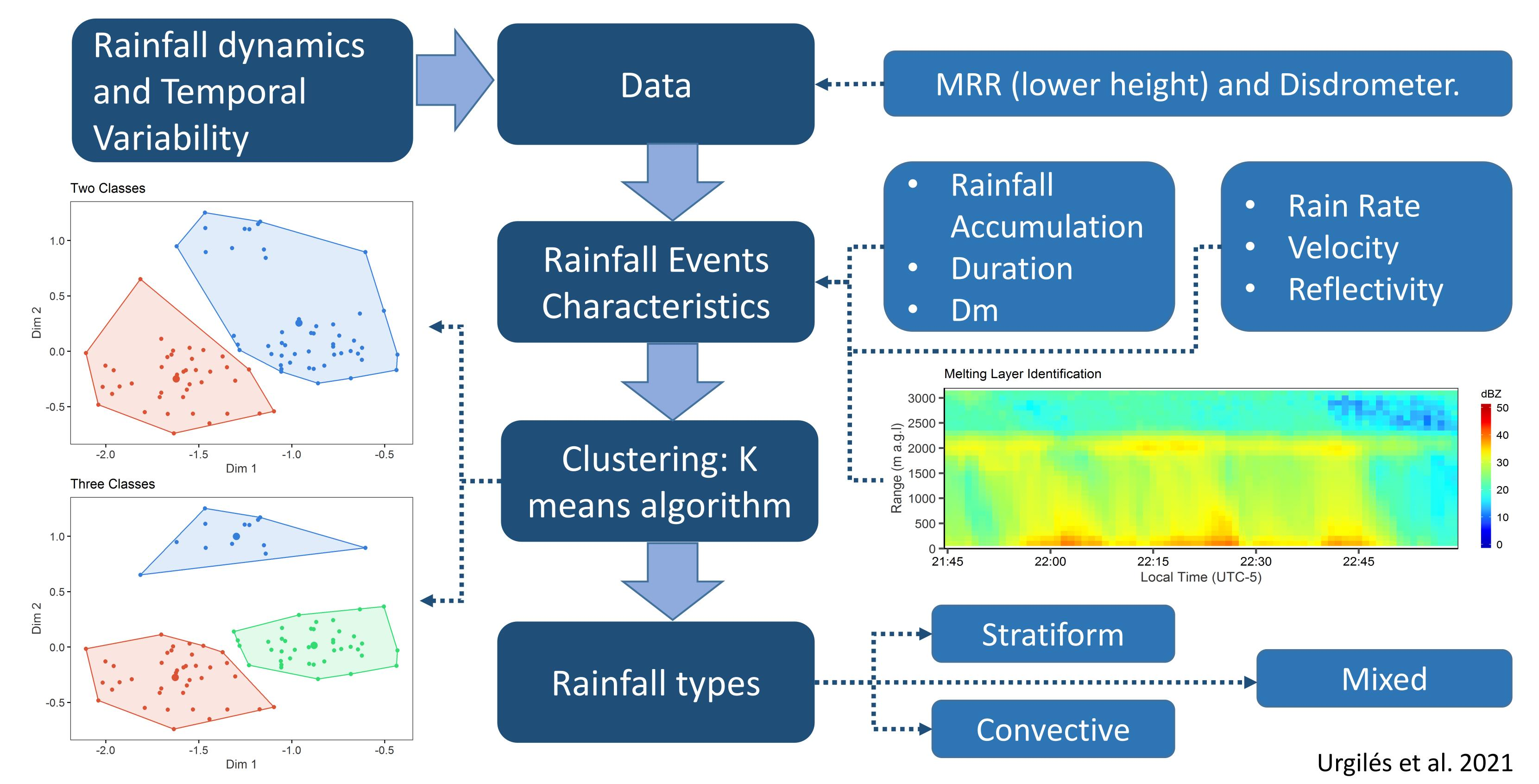
  • Rainfall types were identified by applying a clustering method and thus ensured an objective separation of rainfall events because the classification is based exclusively on the data (i.e., rainfall characteristics). The use of microphysical characteristics, which are not commonly used due to instrument limitations, allowed for the provision of additional insights about each rainfall type.
  • Three rainfall classes were identified in the study area: convective, stratiform, and mixed. The rainfall classes show that the clustering method (k-means) works well to distinguish the different rainfall patterns and identify the rainfall types. The first two main classes, i.e., convective and stratiform, were obtained by first using the method with two classes (k = 2). Here, the two groups showed a clear difference in the features, especially in the mean values of rain rate, velocity, and Dm. In addition, the convective type (class 1) showed rainfall events with shorter duration and higher rain rate than the stratiform type (class 2). The inclusion/exclusion of the Melting Layer feature did not influence the clustering results. Thus, it proves that the other rainfall features are able to properly describe the differences between these two main groups. When using three classes (k = 3), the mixed type (class 3) resulted as a subgroup of one of the main groups (k = 2). So, the convective type remained almost invariable regarding its rainfall characteristics. With respect to the stratiform type and mixed type, their rainfall features are most similar between them. It suggests that the mixed type has a dominant stratiform behavior.
  • Rainfall events with shorter duration of less than 70 min are more frequent in the study area. Furthermore, there is a prevalence of convective rainfall events in March and November, while rainfall events of the stratiform and mixed type are common during all the year.
The findings of this research provide insights about the rainfall dynamics in this tropical mountain setting and show that data with high temporal resolution is necessary to analyze the temporal variability in this area. Furthermore, these rainfall types identified here will be of interest to analyze the vertical profile of rainfall and identify the rainfall formation process. Applications that can benefit from rainfall classification include (i) Numerical Weather Prediction (NWP) verification regarding convective rainfall at high altitudes, (ii) the improvement of quantitative precipitation estimation from scanning weather radar, (iii) the parameterization of cloud microphysical processes in numerical models, and (iv) the analysis of rain-fed soil erosion.
This study allowed for the analysis of the rainfall-event types and their occurrence in the study area. Further analyses on the intraevent rainfall variability is suggested for future investigations.

Author Contributions

Conceptualization, G.U., J.O.-A., R.C.; methodology, G.U., J.O.-A., R.C.; software, G.U.; formal analysis, G.U., J.O.-A., R.C., J.B., K.T.; data curation, G.U., J.O.-A., K.T.; writing—original draft preparation, G.U.; writing—review and editing, J.O.-A., R.C., K.T., J.B.; visualization, G.U.; supervision, J.O.-A., R.C.; project administration, R.C.; funding acquisition, R.C. All authors have read and agreed to the published version of the manuscript.

Funding

This research was funded by the project “High-resolution radar analysis of precipitation extremes in Ecuador and North Peru and implications of the ENSO-dynamics”. It was funded by the German Research Foundation (Deutsche Forschungsgemeinschaft- DFG; DFG GZ.: RO3815/2-1) and the Research Office of the University of Cuenca (DIUC). We want to thank these institutions for their generous funding. The APC was financed by the Marburg University´s Open Access Publishing Fund.

Institutional Review Board Statement

Not applicable

Informed Consent Statement

Not applicable

Data Availability Statement

The data are not publicly available due to university policies because current research is being developed.

Acknowledgments

This manuscript is an outcome of the Maestría en Hidrología mención en Ecohidrología offered by Universidad de Cuenca. We are grateful to the technical staff that contributed to the hydrometeorological monitoring. Furthermore, we would like to thank the three anonymous reviewers whose comments helped to improve the manuscript.

Conflicts of Interest

The authors declare no conflict of interest.

Appendix A

Table A1. The 23 Rainfall events features determined for each event.
NumberFeature NameUnitSymbolInstrument
1Maximum Rain Ratemm h−1RRmaxMRR
2Minimum Rain Ratemm h−1RRminMRR
3Mean Rain Ratemm h−1RRmeanMRR
4Median Rain Ratemm h−1RRmedianMRR
5Rainfall AccumulationmmRaccumMRR
6Maximum Velocitym s−1VmaxMRR
7Minimum Velocitym s−1VminMRR
8Mean Velocitym s−1VmeanMRR
9Median Velocitym s−1VmedianMRR
10Event DurationminutesDurMRR
11Maximum ReflectivitydBZRmaxMRR
12Minimum ReflectivitydBZRminMRR
13Mean ReflectivitydBZRmeanMRR
14Median ReflectivitydBZRmedianMRR
15Melting Layer-MLMRR
16Maximum Liquid Water Contentg m−3LWCmaxMRR
17Minimum Liquid Water Contentg m−3LWCminMRR
18Mean Liquid Water Contentg m−3LWCmeanMRR
19Median Liquid Water Contentg m−3LWCmedianMRR
20Maximum Mean Volume DiametermmDmmaxLPM
21Minimum Mean Volume DiametermmDmminLPM
22Mean Liquid Mean Volume DiametermmDmmeanLPM
23Median Mean Volume DiametermmDmmedianLPM
Figure A1. Cross-correlation matrix between rainfall characteristics. The highlight characteristics are the features selection for the algorithm.
Remotesensing 13 00991 g0a1
Figure A2. Sum of square errors in function of the number of clusters: (a) including ML, (b) excluding ML.
Remotesensing 13 00991 g0a2

References

  1. Chahine, M.T. The hydrological cycle and its influence on climate. Nature 1992, 359, 373. [Google Scholar] [CrossRef]
  2. Mazari, N.; Sharif, H.O.; Xie, H.; Tekeli, A.E.; Zeitler, J.; Habib, E. Rainfall observations and assessment using vertically pointing radar and X-band radar. J. Hydroinform. 2017, 19, 538–557. [Google Scholar] [CrossRef]
  3. Wen, G.; Xiao, H.; Yang, H.; Bi, Y.; Xu, W. Characteristics of summer and winter precipitation over northern China. Atmos. Res. 2017, 197, 390–406. [Google Scholar] [CrossRef]
  4. Orellana-Alvear, J.; Célleri, R.; Rollenbeck, R.; Bendix, J. Analysis of Rain Types and Their Z–R Relationships at Different Locations in the High Andes of Southern Ecuador. J. Appl. Meteorol. Climatol. 2017, 56, 3065–3080. [Google Scholar] [CrossRef]
  5. Buytaert, W.; Célleri, R.; Willems, P.; De Bièvre, B.; Wyseure, G. Spatial and temporal rainfall variability in mountainous areas: A case study from the south Ecuadorian Andes. J. Hydrol. 2006, 329, 413–421. [Google Scholar] [CrossRef]
  6. Celleri, R.; Willems, P.; Buytaert, W.; Feyen, J. Space–time rainfall variability in the Paute basin, Ecuadorian Andes. Hydrol. Process. 2007, 21, 3316–3327. [Google Scholar] [CrossRef]
  7. Rollenbeck, R.; Bendix, J. Rainfall distribution in the Andes of southern Ecuador derived from blending weather radar data and meteorological field observations. Atmos. Res. 2011, 99, 277–289. [Google Scholar] [CrossRef]
  8. Célleri, R.; Buytaert, W.; De Bièvre, B.; Tobon, C.; Crespo, P.; Molina Carpio, J.; Feyen, J. Understanding the Hydrology of Tropical Andean Ecosystems through an Andean Network of Basins. IAHSAISH Publ. 2010, 336, 209–212. [Google Scholar] [CrossRef]
  9. Metek. MRR Physical Basics, Valid for MRR Service Version 5.2.0.1; Technical Manual; METEK: Elmshorn, Germany, 2009. [Google Scholar]
  10. 10. Thies Clima. Instructions for use: Laser Precipitation Monitor 5.4110.xx.x00 V2.2xSTD. Thies Clima Tech. Rep. 2007, 1–52.
  11. Das, S.; Shukla, A.K.; Maitra, A. Investigation of vertical profile of rain microstructure at Ahmedabad in Indian tropical region. Adv. Space Res. 2010, 45, 1235–1243. [Google Scholar] [CrossRef]
  12. Endries, J.L.; Perry, L.B.; Yuter, S.E.; Seimon, A.; Andrade-Flores, M.; Winkelmann, R.; Quispe, N.; Rado, M.; Montoya, N.; Velarde, F.; et al. Radar-observed characteristics of precipitation in the tropical high andes of Southern Peru and Bolivia. J. Appl. Meteorol. Climatol. 2018, 57, 1441–1458. [Google Scholar] [CrossRef]
  13. Sreekanth, T.S.; Varikoden, H.; Resmi, E.A.; Kumar, G.M. Classification and seasonal distribution of rain types based on surface and radar observations over a tropical coastal station. Atmos. Res. 2019, 218, 90–98. [Google Scholar] [CrossRef]
  14. Seidel, J.; Trachte, K.; Orellana-Alvear, J.; Figueroa, R.; Célleri, R.; Bendix, J.; Fernandez, C.; Huggel, C. Precipitation Characteristics at Two Locations in the Tropical Andes by Means of Vertically Pointing Micro-Rain Radar Observations. Remote Sens. 2019, 11, 2985. [Google Scholar] [CrossRef] [Green Version]
  15. Zwiebel, J.; Van Baelen, J.; Anquetin, S.; Pointin, Y.; Boudevillain, B. Impacts of orography and rain intensity on rainfall structure. The case of the HyMeX IOP7a event. Q. J. R. Meteorol. Soc. 2016, 142, 310–319. [Google Scholar] [CrossRef]
  16. Bendix, J.; Rollenbeck, R.; Reudenbach, C. Diurnal patterns of rainfall in a tropical Andean valley of southern Ecuador as seen by a vertically pointing K-band Doppler radar. Int. J. Climatol. 2006, 26, 829–846. [Google Scholar] [CrossRef]
  17. Prat, O.P.; Barros, A.P. Ground observations to characterize the spatial gradients and vertical structure of orographic precipitation—Experiments in the inner region of the Great Smoky Mountains. J. Hydrol. 2010, 391, 141–156. [Google Scholar] [CrossRef]
  18. Bellon, A.; Lee, G.W.; Zawadzki, I. Error statistics of VPR corrections in stratiform precipitation. J. Appl. Meteorol. 2005, 44, 998–1015. [Google Scholar] [CrossRef] [Green Version]
  19. Das, S.; Maitra, A. Vertical profile of rain: Ka band radar observations at tropical locations. J. Hydrol. 2016, 534, 31–41. [Google Scholar] [CrossRef]
  20. Li, Y.; Liu, X.; Wu, Y.; Hu, S. Characteristics and Small-Scale Variations of Raindrop Size Distribution over the Yangtze River Delta in East China. J. Hydrol. Eng. 2020, 25, 5020010. [Google Scholar] [CrossRef]
  21. Llasat, M.-C. An objective classification of rainfall events on the basis of their convective features: Application to rainfall intensity in the northeast of spain. Int. J. Climatol. 2001, 21, 1385–1400. [Google Scholar] [CrossRef]
  22. Thurai, M.; Gatlin, P.N.; Bringi, V.N. Separating stratiform and convective rain types based on the drop size distribution characteristics using 2D video disdrometer data. Atmos. Res. 2016, 169, 416–423. [Google Scholar] [CrossRef]
  23. Caracciolo, C.; Porcù, F.; Prodi, F. Precipitation classification at mid-latitudes in terms of drop size distribution parameters. Adv. Geosci. 2008, 16, 11–17. [Google Scholar] [CrossRef] [Green Version]
  24. Biggerstaff, M.I.; Listemaa, S.A. An improved scheme for convective/stratiform echo classification using radar reflectivity. J. Appl. Meteorol. 2000, 39, 2129–2150. [Google Scholar] [CrossRef]
  25. Kunhikrishnan, P.K.; Sivaraman, B.R.; Kumar, N.V.P.K.; Alappattu, D.P. Rain observations with micro rain radar (MRR) over Thumba. Proc. SPIE 2006, 6408. [Google Scholar] [CrossRef]
  26. Dilmi, M.D.; Mallet, C.; Barthes, L.; Chazottes, A. Data-driven clustering of rain events: Microphysics information derived from macro-scale observations. Atmos. Meas. Tech. 2017, 10, 1557–1574. [Google Scholar] [CrossRef] [Green Version]
  27. dos Santos, J.C.N.; de Andrade, E.M.; Medeiros, P.H.A.; Guerreiro, M.J.S.; de Queiroz Palácio, H.A. Effect of Rainfall Characteristics on Runoff and Water Erosion for Different Land Uses in a Tropical Semiarid Region. Water Resour. Manag. 2017, 31, 173–185. [Google Scholar] [CrossRef]
  28. Fang, N.-F.; Shi, Z.-H.; Li, L.; Guo, Z.-L.; Liu, Q.; Ai, L. The effects of rainfall regimes and land use changes on runoff and soil loss in a small mountainous watershed. CATENA 2012, 99, 1–8. [Google Scholar] [CrossRef]
  29. Peng, T.; Wang, S. Effects of land use, land cover and rainfall regimes on the surface runoff and soil loss on karst slopes in southwest China. CATENA 2012, 90, 53–62. [Google Scholar] [CrossRef]
  30. Coltorti, M.; Ollier, C. Geomorphic and tectonic evolution of the Ecuadorian Andes. Geomorphology 2000, 32, 1–19. [Google Scholar] [CrossRef]
  31. Córdova, M.; Célleri, R.; Shellito, C.J.; Orellana-Alvear, J.; Abril, A.; Carrillo-Rojas, G. Near-Surface Air Temperature Lapse Rate Over Complex Terrain in the Southern Ecuadorian Andes: Implications for Temperature Mapping. Arct. Antarct. Alp. Res. 2016, 48, 673–684. [Google Scholar] [CrossRef] [Green Version]
  32. Poveda, G.; Mesa, O.J. Feedbacks between Hydrological Processes in Tropical South America and Large-Scale Ocean–Atmospheric Phenomena. J. Clim. 1997, 10, 2690–2702. [Google Scholar] [CrossRef]
  33. Campozano, L.; Trachte, K.; Célleri, R.; Samaniego, E.; Bendix, J.; Albuja, C.; Mejia, J.F. Climatology and Teleconnections of Mesoscale Convective Systems in an Andean Basin in Southern Ecuador: The Case of the Paute Basin. Adv. Meteorol. 2018, 2018, 1–13. [Google Scholar] [CrossRef] [PubMed]
  34. Žagar, N.; Skok, G.; Tribbia, J. Climatology of the ITCZ derived from ERA Interim reanalyses. J. Geophys. Res. 2011, 116. [Google Scholar] [CrossRef] [Green Version]
  35. Vuille, M.; Bradley, R.S.; Keimig, F. Climate Variability in the Andes of Ecuador and Its Relation to Tropical Pacific and Atlantic Sea Surface Temperature Anomalies. J. Clim. 2000, 13, 2520–2535. [Google Scholar] [CrossRef]
  36. Peters, G.; Fischer, B.; Andersson, T. Rain observations with a vertically looking Micro Rain Radar (MRR). Boreal Environ. Res. 2002, 7, 353–362. [Google Scholar]
  37. Löffler-Mang, M.; Kunz, M.; Schmid, W. On the Performance of a Low-Cost K-Band Doppler Radar for Quantitative Rain Measurements. J. Atmos. Ocean. Technol. 1999, 16, 379–387. [Google Scholar] [CrossRef]
  38. Wang, H.; Lei, H.; Yang, J. Microphysical processes of a stratiform precipitation event over eastern China: Analysis using micro rain radar data. Adv. Atmos. Sci. 2017, 34, 1472–1482. [Google Scholar] [CrossRef]
  39. Frasson, R.; Cunha, L.; Krajewski, W. Assessment of the Thies optical disdrometer performance. Atmos. Res. 2011, 101, 237–255. [Google Scholar] [CrossRef]
  40. Sarkar, T.; Das, S.; Maitra, A. Assessment of different raindrop size measuring techniques: Inter-comparison of Doppler radar, impact and optical disdrometer. Atmos. Res. 2015, 160, 15–27. [Google Scholar] [CrossRef]
  41. Friedrich, K.; Higgins, S.; Masters, F.J.; Lopez, C.R. Articulating and Stationary PARSIVEL Disdrometer Measurements in Conditions with Strong Winds and Heavy Rainfall. J. Atmos. Ocean. Technol. 2013, 30, 2063–2080. [Google Scholar] [CrossRef]
  42. Tokay, A.; Hartmann, P.; Battaglia, A.; Gage, K.S.; Clark, W.L.; Williams, C.R. A field study of reflectivity and Z-R relations using vertically pointing radars and disdrometers. J. Atmos. Ocean. Technol. 2009, 26, 1120–1134. [Google Scholar] [CrossRef]
  43. Adirosi, E.; Baldini, L.; Tokay, A. Rainfall and DSD Parameters Comparison between Micro Rain Radar, Two-Dimensional Video and Parsivel2 Disdrometers, and S-Band Dual-Polarization Radar. J. Atmos. Ocean. Technol. 2020, 37, 621–640. [Google Scholar] [CrossRef]
  44. Rollenbeck, R.; Bendix, J.; Fabian, P.; Boy, J.; Dalitz, H.; Emck, P.; Oesker, M.; Wilcke, W. Comparison of Different Techniques for the Measurement of Precipitation in Tropical Montane Rain Forest Regions. J. Atmos. Ocean. Technol. 2007, 24, 156–168. [Google Scholar] [CrossRef]
  45. Adirosi, E.; Baldini, L.; Roberto, N.; Gatlin, P.; Tokay, A. Improvement of vertical profiles of raindrop size distribution from micro rain radar using 2D video disdrometer measurements. Atmos. Res. 2016, 169, 404–415. [Google Scholar] [CrossRef]
  46. Beard, K. V Terminal Velocity and Shape of Cloud and Precipitation Drops Aloft. J. Atmos. Sci. 1976, 33, 851–864. [Google Scholar] [CrossRef] [Green Version]
  47. Dunkerley, D. Identifying individual rain events from pluviograph records: A review with analysis of data from an Australian dryland site. Hydrol. Process. 2008, 22, 5024–5036. [Google Scholar] [CrossRef]
  48. Coutinho, J.V.; Almeida, C.D.N.; Leal, A.M.F.; Barbosa, L.R. Characterization of sub-daily rainfall properties in three raingauges located in northeast Brazil. Proc. Int. Assoc. Hydrol. Sci. 2014, 364, 345–350. [Google Scholar] [CrossRef]
  49. Marshall, J.S.; Palmer, W.M.K. The Distribution of Raindrops with size. J. Meteorol. 1948, 5, 165–166. [Google Scholar] [CrossRef]
  50. Testud, J.; Oury, S.; Black, R.A.; Amayenc, P.; Dou, X. The concept of “normalized” distribution to describe raindrop spectra: A tool for cloud physics and cloud remote sensing. J. Appl. Meteorol. 2001, 40, 1118–1140. [Google Scholar] [CrossRef]
  51. Jash, D.; Resmi, E.A.; Unnikrishnan, C.K.; Sumesh, R.K.; Sreekanth, T.S.; Sukumar, N.; Ramachandran, K.K. Variation in rain drop size distribution and rain integral parameters during southwest monsoon over a tropical station: An inter-comparison of disdrometer and Micro Rain Radar. Atmos. Res. 2019, 217, 24–36. [Google Scholar] [CrossRef]
  52. Zhou, L.; Dong, X.; Fu, Z.; Wang, B.; Leng, L.; Xi, B.; Cui, C. Vertical Distributions of Raindrops and Z-R Relationships Using Microrain Radar and 2-D-Video Distrometer Measurements During the Integrative Monsoon Frontal Rainfall Experiment (IMFRE). J. Geophys. Res. Atmos. 2020, 125, e2019JD031108. [Google Scholar] [CrossRef] [Green Version]
  53. Cha, J.-W.; Chang, K.-H.; Yum, S.S.; Choi, Y.-J. Comparison of the bright band characteristics measured by Micro Rain Radar (MRR) at a mountain and a coastal site in South Korea. Adv. Atmos. Sci. 2009, 26, 211–221. [Google Scholar] [CrossRef]
  54. Klaassen, W. Radar Observations and Simulation of the Melting Layer of Precipitation. J. Atmos. Sci. 1988, 45, 3741–3753. [Google Scholar] [CrossRef]
  55. Fabry, F.; Zawadzki, I. Long-Term Radar Observations of the Melting Layer of Precipitation and Their Interpretation. J. Atmos. Sci. 1995, 52, 838–851. [Google Scholar] [CrossRef]
  56. Abu Abbas, O. Comparisons Between Data Clustering Algorithms. Int. Arab. J. Inf. Technol. 2008, 5, 320–325. [Google Scholar]
  57. Jain, A. Data Clustering: 50 Years Beyond K-Means. Pattern Recognit. Lett. 2010, 31, 651–666. [Google Scholar] [CrossRef]
  58. Steinley, D. K-means clustering: A half-century synthesis. Br. J. Math. Stat. Psychol. 2006, 59, 1–34. [Google Scholar] [CrossRef] [PubMed] [Green Version]
  59. Löwe, R.; Madsen, H.; McSharry, P. Objective Classification of Rainfall in Northern Europe for Online Operation of Urban Water Systems Based on Clustering Techniques. Water 2016, 8, 87. [Google Scholar] [CrossRef] [Green Version]
  60. Hartigan, J.A.; Wong, M.A. Algorithm AS 136: A K-Means Clustering Algorithm. Appl. Stat. 1979, 28, 100. [Google Scholar] [CrossRef]
  61. Liu, Y.; Liu, L. Rainfall feature extraction using cluster analysis and its application on displacement prediction for a cleavage-parallel landslide in the Three Gorges Reservoir area. Nat. Hazards Earth Syst. Sci. Discuss. 2016, 2016, 1–15. [Google Scholar] [CrossRef] [Green Version]
  62. Guyon, I.; Elisseeff, A. An introduction to variable and feature selection. J. Mach. Learn. Res. 2003, 3, 1157–1182. [Google Scholar]
  63. Milligan, G.W.; Cooper, M.C. A study of standardization of variables in cluster analysis. J. Classif. 1988, 5, 181–204. [Google Scholar] [CrossRef]
  64. Milligan, G.W.; Cooper, M.C. An examination of procedures for determining the number of clusters in a data set. Psychometrika 1985, 50, 159–179. [Google Scholar] [CrossRef]
  65. Mouton, J.P.; Ferreira, M.; Helberg, A.S.J. A comparison of clustering algorithms for automatic modulation classification. Expert Syst. Appl. 2020, 151, 113317. [Google Scholar] [CrossRef]
  66. Abdi, H.; Williams, L.J. Principal component analysis. Wiley Interdiscip. Rev. Comput. Stat. 2010, 2, 433–459. [Google Scholar] [CrossRef]
  67. Wold, S.; Esbensen, K.; Geladi, P. Principal component analysis. Chemom. Intell. Lab. Syst. 1987, 2, 37–52. [Google Scholar] [CrossRef]
  68. Padrón, R.S.; Wilcox, B.P.; Crespo, P.; Célleri, R. Rainfall in the Andean Páramo: New Insights from High-Resolution Monitoring in Southern Ecuador. J. Hydrometeorol. 2015, 16, 985–996. [Google Scholar] [CrossRef]
  69. Tokay, A.; Short, D.A.; Williams, C.R.; Ecklund, W.L.; Gage, K.S. Tropical Rainfall Associated with Convective and Stratiform Clouds: Intercomparison of Disdrometer and Profiler Measurements. J. Appl. Meteorol. 1999, 38, 302–320. [Google Scholar] [CrossRef]
  70. Bringi, V.N.; Chandrasekar, V.; Hubbert, J.; Gorgucci, E.; Randeu, W.L.; Schoenhuber, M. Raindrop Size Distribution in Different Climatic Regimes from Disdrometer and Dual-Polarized Radar Analysis. J. Atmos. Sci. 2003, 60, 354–365. [Google Scholar] [CrossRef]
Figure 1. Study site in the southern Ecuador; the diamond indicates the location of instruments.
Remotesensing 13 00991 g001
Figure 2. Correlation between rainfall recorded by the Micro Rain Radar (MRR) and Laser Precipitation Monitor (LPM) data at 30-min accumulation. The solid line denotes the regression line, the dashed line denotes the bisector line, and R2 is the determination coefficient.
Remotesensing 13 00991 g002
Figure 3. Violin plots show the frequency distribution of rainfall event duration per month at Balzay. n is the number of events and the gray point represents the mean value.
Remotesensing 13 00991 g003
Figure 4. Event with a clear bright band on 21 March 2019: (a) reflectivity profile (dBZ), (b) vertical fall velocity (m s−1), (c) rain rate at range of 100 m a.g.l (mm h−1).
Remotesensing 13 00991 g004
Figure 5. Event with intermittent bright band on 26 December 2017: (a) reflectivity profile (dBZ), (b) vertical fall velocity (m s−1), (c) rain rate at range of 100 m a.g.l (mm h−1). White color in (a), represents missing data.
Remotesensing 13 00991 g005
Figure 6. Event without bright band on 29 January 2019: (a) reflectivity profile (dBZ), (b) vertical fall velocity (m s−1), (c) rain rate at range of 100 m a.g.l (mm h−1). White color in (a), represents missing data.
Remotesensing 13 00991 g006
Figure 7. Standardized features using the range method.
Remotesensing 13 00991 g007
Figure 8. The classified rainfall events based on cluster analysis: (a) two classes (with Melting Layer—ML feature), (b) two classes (without ML feature), (c) three classes (with ML feature), (d) three classes (without ML feature). Cl1, Cl2, Cl3 are the number of events per each class.
Remotesensing 13 00991 g008
Figure 9. Boxplots of variables: (a) two classes, (b) three classes.
Remotesensing 13 00991 g009
Figure 10. Monthly event percentage for two classes: (a) with ML feature, (b) without ML feature. Events for three classes: (c) with ML feature, (d) without ML feature.
Remotesensing 13 00991 g010
Table 1. Features selected for the cluster analysis.
NumberVariable NameUnitSymbol
1Maximum Rain Ratemm h−1RRmax
2Minimum Rain Ratemm h−1RRmin
3Mean Rain Ratemm h−1RRmean
4Rainfall AccumulationmmRaccum
5Maximum Velocitym s−1Vmax
6Minimum Velocitym s−1Vmin
7Mean Velocitym s−1Vmean
8Event DurationminutesDur
9Melting Layer-ML
10Maximum Mean Volume DiametermmDmmax
11Minimum Mean Volume DiametermmDmmin
12Mean Liquid Mean Volume DiametermmDmmean
Table 2. Summary of rainfall features thresholds of Tropical Zones.
Feature (Units)AuthorLocationRainfall
Classification
Value
Rain Rate (mm h−1)Tokay, (1999)Marine
Tropics
Convective>10
Stratiform≈1.86
Bendix, (2006)Mountains South
Ecuador
Mixed≈2.4
Das and Maitra, (2016)Tropical
Locations
Convective8–12
Stratiform2–5
This studyTropical
Andes
Class 1 (k = 2)14.86 ± 0.20
Class 2 (k = 2)6.55 ± 0.08
Class 1 (k = 3)15.08 ± 0.32
Class 2 (k = 3)5.43 ± 1.06
Class 3 (k = 3)7.27 ± 0.14
Dm (mm)Seidel, (2019)Tropical
Andes
Convective≈1.66
Stratiform≈1.07
This studyTropical
Andes
Class 1 (k = 2)1.55 ± 0.01
Class 2 (k = 2)1.09 ± 0.01
Class 1 (k = 3)1.57 ± 0.02
Class 2 (k = 3)1.1 ± 0.05
Class 3 (k = 3)1.1 ± 0.01
Publisher’s Note: MDPI stays neutral with regard to jurisdictional claims in published maps and institutional affiliations.

