Mapping Paddy Rice with Sentinel-1/2 and Phenology-, Object-Based Algorithm—A Implementation in Hangjiahu Plain in China Using GEE Platform

Abstract

In tropical/subtropical monsoon regions, accurate rice mapping is hampered by the following factors: (1) The frequent occurrence of clouds in such areas during the rice-growing season interferes strongly with optical remote sensing observations; (2) The agro-landscape in such regions is fragmented and scattered. Rice maps produced using low spatial resolution data cannot well delineate the detailed distribution of rice, while pixel-based mapping using medium and high resolutions has significant salt-and-pepper noise. (3) The cropping system is complex, and rice has a rotation schedule with other crops. Therefore, the Phenology-, Object- and Double Source-based (PODS) paddy rice mapping algorithm is implemented, which consists of three steps: (1) object extraction from multi-temporal 10-m Sentinel-2 images where the extracted objects (fields) are the basic classification units; (2) specifying the phenological stage of transplanting from Savitzky–Golay filtered enhanced vegetation index (EVI) time series using the PhenoRice algorithm; and (3) the identification of rice objects based on flood signal detection from time-series microwave and optical signals of the Sentinel-1/2. This study evaluated the potential of the combined use of the Sentinel-1/2 mission on paddy rice mapping in monsoon regions with the Hangzhou-Jiaxin-Huzhou (HJH) plain in China as the case study. A cloud computing approach was used to process the available Sentinel-1/2 imagery from 2019 and MODIS images from 2018 to 2020 in the HJH plain on the Google Earth Engine (GEE) platform. An accuracy assessment showed that the resultant object-based paddy rice map has a high accuracy with a producer (user) accuracy of 0.937 (0.926). The resultant 10-m paddy rice map is expected to provide unprecedented detail, spatial distribution, and landscape patterns for paddy rice fields in monsoon regions.

1. Introduction

Rice feeds more than half of the global human population [1] with more than 90% of rice production being in Asia [2]. Moreover, the International Food Policy Research Institute suggests that the demand for rice increases by 1.8% per year. Therefore, obtaining information on the rice location and distribution is important for food security and water use. Field survey-based agricultural statistical methods, which is the conventional approach to determine rice planting areas, is time- and labor-intensive. Tabular data obtained from this method lacks explicit spatial distribution information, and the data may be altered in regions where agriculture subsidies are provided. In contrast, remote sensing methods are an efficient and reliable approach to obtain spatially explicit and objective data. The main data sources are optical and synthetic aperture radar (SAR). Optical data provide spectral information of the surface and reflects the biochemical characteristics of objects. However, the nature of passive imaging and its short wavelength means it is easily affected by atmospheric factors, such as clouds and cloud shadows. SAR data provide backscattering information in different polarizations for surface objects and captures their physical characteristics, such as spatial structure and dielectric properties. The nature of active imaging and its long wavelength has all-weather and day-and-night observation capabilities.

Dong and Xiao [3] reviewed the evolution of remote sensing methods for paddy rice mapping from the 1980s through 2015, in which the approaches were divided into four categories: (1) reflectance data and image statistics; (2) vegetation indices (VIs) and enhanced image statistics; (3) VI or radar backscatter-based temporal analysis; and (4) phenology through remote sensing recognition of key growth phases. The first and second categories use supervised or unsupervised algorithms, such as the maximum likelihood classifier, random forest, and support vector machine, which involve human intervention in sample collection or cluster labeling to build the models. The feasibility of such image- and statistics-based approaches has been limited to specific regions or periods due to the inherent spectral variability, which makes it difficult to perform large-scale monitoring of crop information over multiple years [4]. An example of the third category is rice cropping system maps as produced by Gumma [5] for South Asia. This method has generated accurate maps over wide areas, but its application to other regions would involve an additional round of time-consuming operator analysis and decision making for the classification, grouping, and labeling phases.

The fourth approach defines a series of detection criteria based on the well-known temporal characteristics of rice cultivation. One of the most cited methods for rice detection in the fourth approach was proposed using the Spot Vegetation (VGT) data [6] and later MODIS data [7] to map rice flooding and rice cultivated areas in China and South and Southeast Asia [8]. This method is based on the detection of agronomic (i.e., deliberate) flooding of rice fields before the crop is established and its subsequent rapid growth within a fixed time after flooding. As these two characteristics are common to many rice cultivation practices (with the exceptions of upland rice, deepwater rice, dry direct-seeded rice, and other relatively minor rice ecosystems or rice management practices), this approach has the potential for operational monitoring of rice-cultivated areas at regional scales. However, demonstrations of this method have revealed that false positives can occur when applied in ecosystems different from those where it was originally developed [9] or when external knowledge of the local crop calendar and agro-practices are not considered [10]. In temperate regions where the temperature is the primary factor limiting rice growth, a signal detection time window during the transplanting phase of rice can be determined from the time-series temperature data to filter false signals from outside the window [11]. Apart from temperature constraints, the choice of when to establish a crop is driven by several other factors, such as water availability in water-limited environments, temporal variability in water salinity, risk of submergence, or combinations therein [12]. Therefore, it is possible to map the potential growing season for rice based on climatic suitability parameters. However, in South, Southeast, and East Asia, where 90% of the world’s rice is produced, the subtropical and tropical temperatures, the abundance of water during the monsoon season, and the increasing reliance on irrigation in the dry season have allowed rice to be grown at nearly any time of year across the region [13].

The MODIS satellite is characterized by its hyper-temporal resolution and has become the primary data source for vegetation phenology retrieval. Several algorithms have been proposed based on this system. For example, Sakamoto et al. [14,15] used wavelet analysis to extract seasonality information from multi-temporal MODIS imagery for rice crops in Japan and along the Mekong delta. Nguyen et al. [16] and Asilo et al. [17] used labeling and grouping of unsupervised classifications with VGT data in the Mekong delta and MODIS data in the Philippines, respectively, to generate rice crop calendars. Tornos et al. [18] studied the temporal characteristics of rice cropping systems in Spain and demonstrated that time-series data of vegetation indices can help analyze changes in flooding periods (hydroperiod). Boschetti [19] presented a rule-based algorithm called PhenoRice for the automated extraction of temporal information on rice crops using MODIS data. PhenoRice has been applied extensively in research [4,20], and the results showed that this could effectively estimate temporal information.

In addition to complex cropping systems, many regions in South and Southeast Asia are characterized as fragmented landscapes due to their complex terrain and frequent cloud coverage during the rice-growing season as induced by monsoons. Current applications of such phenology-based approaches generally use coarse-resolution MODIS data, which involves mixed pixel issues in Asia where smallholders constitute the majority of paddy rice agriculture [3]. For fragmented agro-landscapes, low-resolution satellite imagery may significantly over-estimate or under-estimate cropland areas [21]. The free release of Landsat archival data and the launch of Landsat 8 and Sentinel-2 provide unprecedented opportunities to map paddy rice in fragmented landscapes with a higher spatial resolution; however, the salt-and-pepper effect from the enhanced spatial resolution is another issue in pixel-based classification. Classifying crops on a per-field (object-based) approach is known to produce better results than per-pixel methods.

Several remote sensing approaches to determine the extent of cropland have been explored. It has been proved that the use of multi-temporal images with higher spatial resolution generally achieves better performance compared with the use of mono-temporal images or images of lower resolution [22,23]. Watkins [24] evaluated several Earth observation methodologies to automatically delineate crop field boundaries from multi-temporal Sentinel-2 imagery, which uses edge detection as applied to multiple images acquired during the growing season along with image segmentation to delimit agricultural fields, orchards, and vineyards. A promising result was achieved by applying the Canny edge detector to multiple Sentinel-2 images [24]. However, the usage of multi-temporal high spatial resolution data causes an explosive increase in data volume, meaning the size of study area is limited by data storage and processing capability of the local general-purpose computer.

Due to frequent cloud coverage, SAR-based images have gained increasing attention recently as they are not affected by clouds or illumination conditions. The SAR backscatter mechanism for fields changes from surface reflection to specular reflection as indicated by a rapid decrease in the backscatter coefficient when regions are flooded due to natural or agro-practice flooding. Therefore, extensive research has been conducted on mapping the extent of paddy rice [25,26] or flooded regions [27] using this fact. In recent studies, effectively combining optical and microwave data has become a research hotspot as this can often provide higher precision than single data sources. Data availability has been greatly improved by the implementation of the Copernicus Programme, which is an Earth observation initiative that provides unprecedented levels of observational capabilities through the operation of recently launched satellites (called Sentinels). The Sentinel-1 data are part of the first global open-access SAR dataset, and the Sentinel-2 constellation provides a significant increase in the observational capacity compared with other satellites, such as Landsat, due to its large number (13) of spectral bands, high (10–60 m) spatial resolutions, and short (five-day) revisit times. The objectives of this research are to develop a paddy rice mapping algorithm that exploits the great Earth observation capability offered by Sentinel-1/2 based on the temporal characteristics of paddy rice fields. The algorithm (i) accommodates fragmentation of agro-landscapes, (ii) achieves good performance in regions frequently covered by clouds, and (iii) deals with complex cropping systems. Some improvements are made on Dong’s pixel- and phenology-based rice mapping algorithm [11]: for rice phenology, MODIS temperature time series is substituted by MODIS vegetation index time series, to which PhenoRice algorithm [19] is applied; for object-based classification, an edge-based image segmentation algorithm is applied to multiple-temporal Sentinel-2 images to extract objects (fields) [20]. The improved algorithm is named the Phenology-, Object-, and Double Source-based algorithm (PODS).

2. Study Area and Datasets

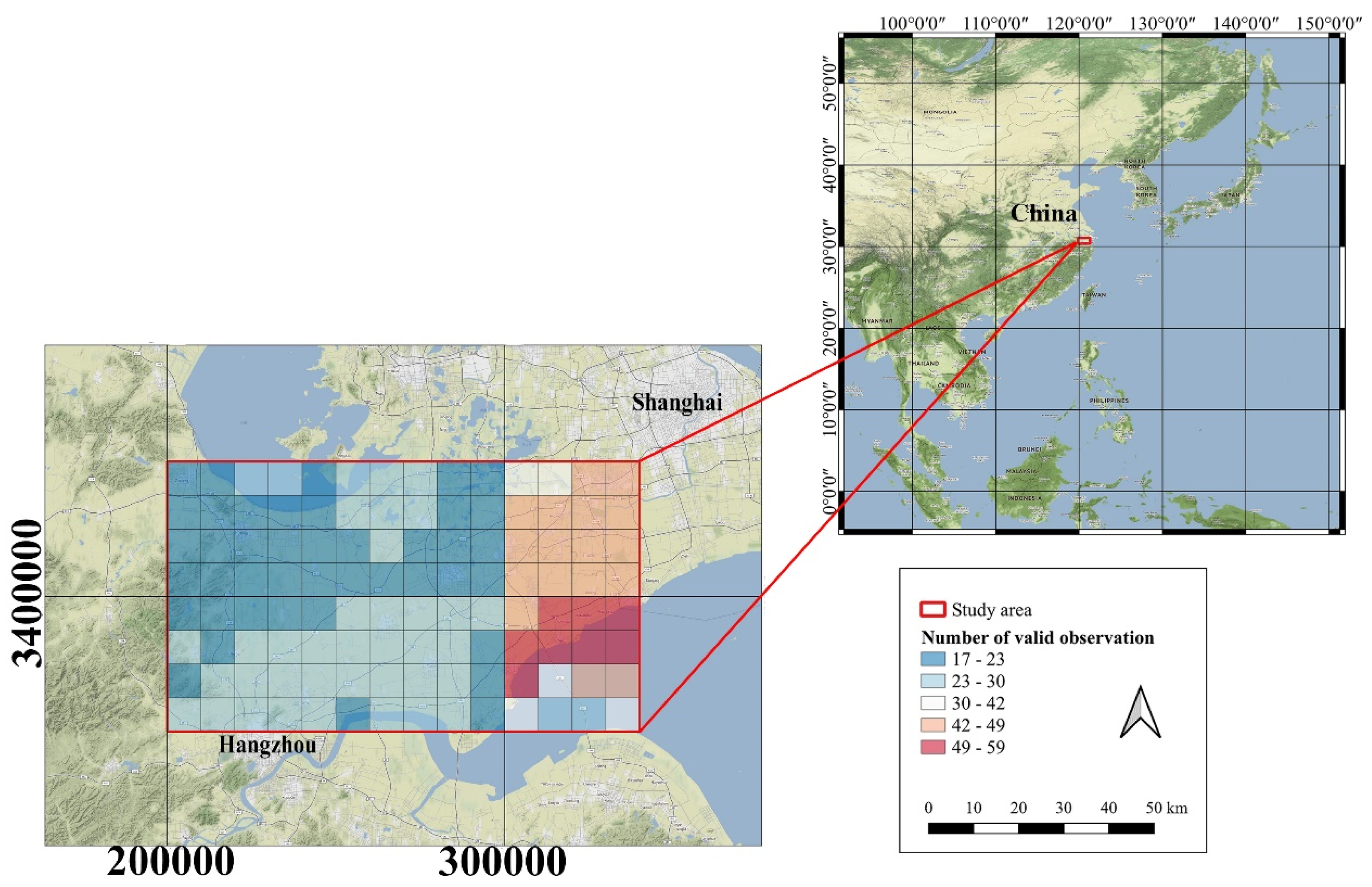
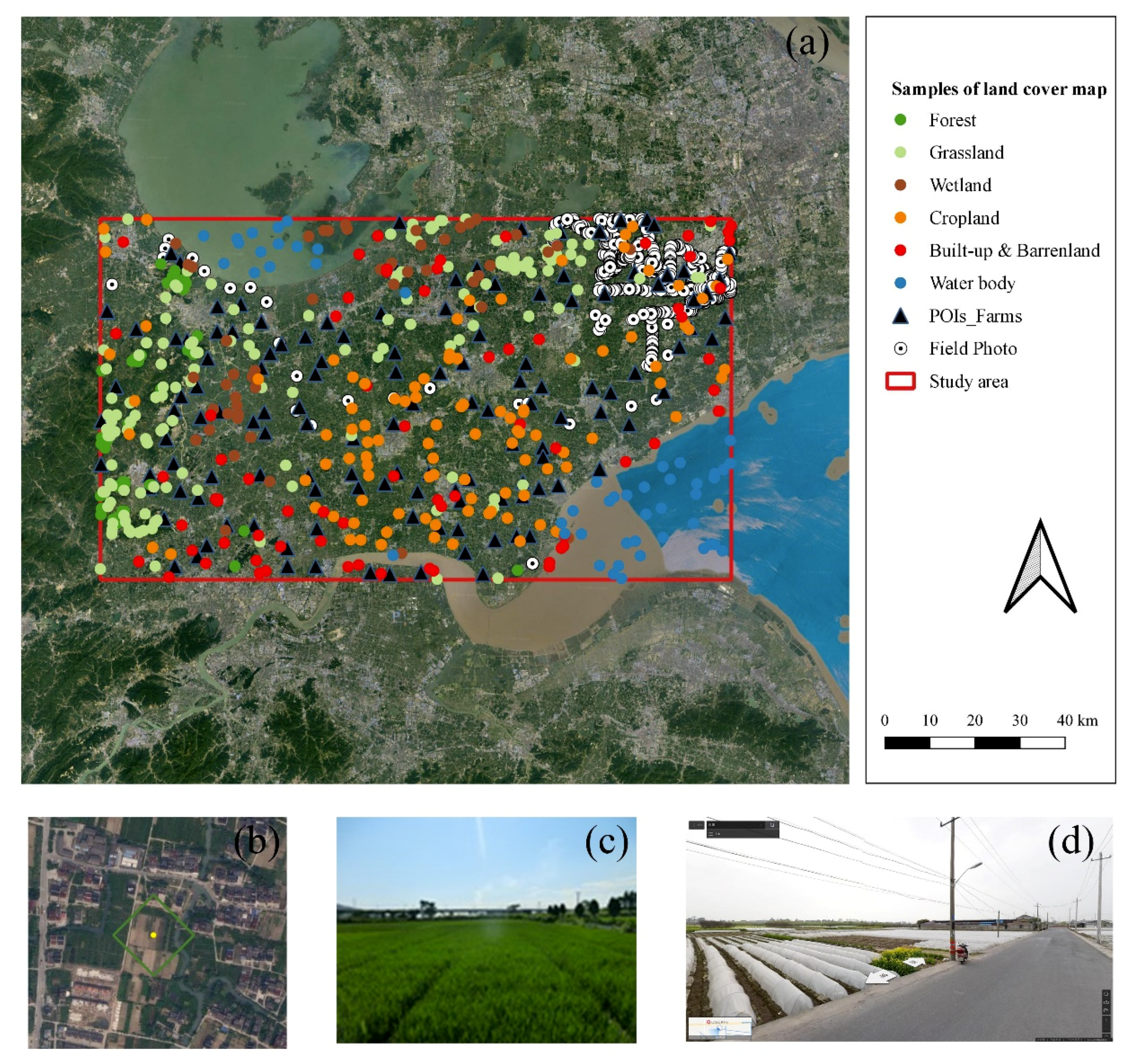
2.1. Study Area

The Hangzhou–Jiaxing–Huzhou (HJH) Plain, or Hangjiahu Plain, is the largest plain in Zhejiang province, China and is an integral part of the Yangtze Delta. It comprises an area of 7620 km² (2940 sq. mi.) and is bound by Lake Tai to the north, the Qiantang River/Hangzhou Bay to the south, and the Tianmu Mountains to the west. It includes all of the prefecture-level city of Jiaxing, most of Huzhou, and the northeastern part of Hangzhou. It has a humid subtropical climate (Köppen Cfa) that is influenced by East Asian monsoons with cool winters and very hot and humid summers. The topography is generally low-lying and flat at around a 3-m elevation, though it is slightly higher to the south and east with lower slopes towards Lake Tai. Its river and canal network, including the Grand Canal, is 12.7 km per km² (20.4 mi per sq. mi.), which is the densest area in China.

The HJH Plain is the primary rice production region in Zhejiang province, which belongs to the single cropping japonica rice area [28]. The growing period with temperatures above 10 °C was 217–222 d, and the cumulative temperature was 4772–4960 °C. The rice-growing season is roughly between May and October, and the annual precipitation is 734.3–905.0 mm. The rice area accounts for 28.1% of all rice planting in Zhejiang province. The region is dominated by single cropping rice, accounting for 90.4% of all rice, while the areas of early and late rice account for 1.7% and 7.9%, respectively.

2.2. Dataset and Preprocessing

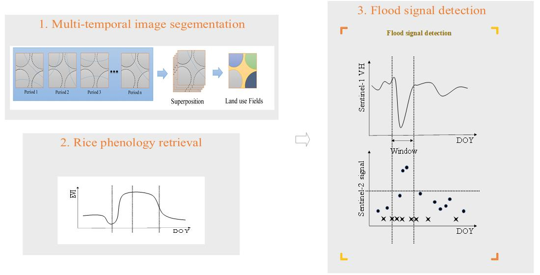
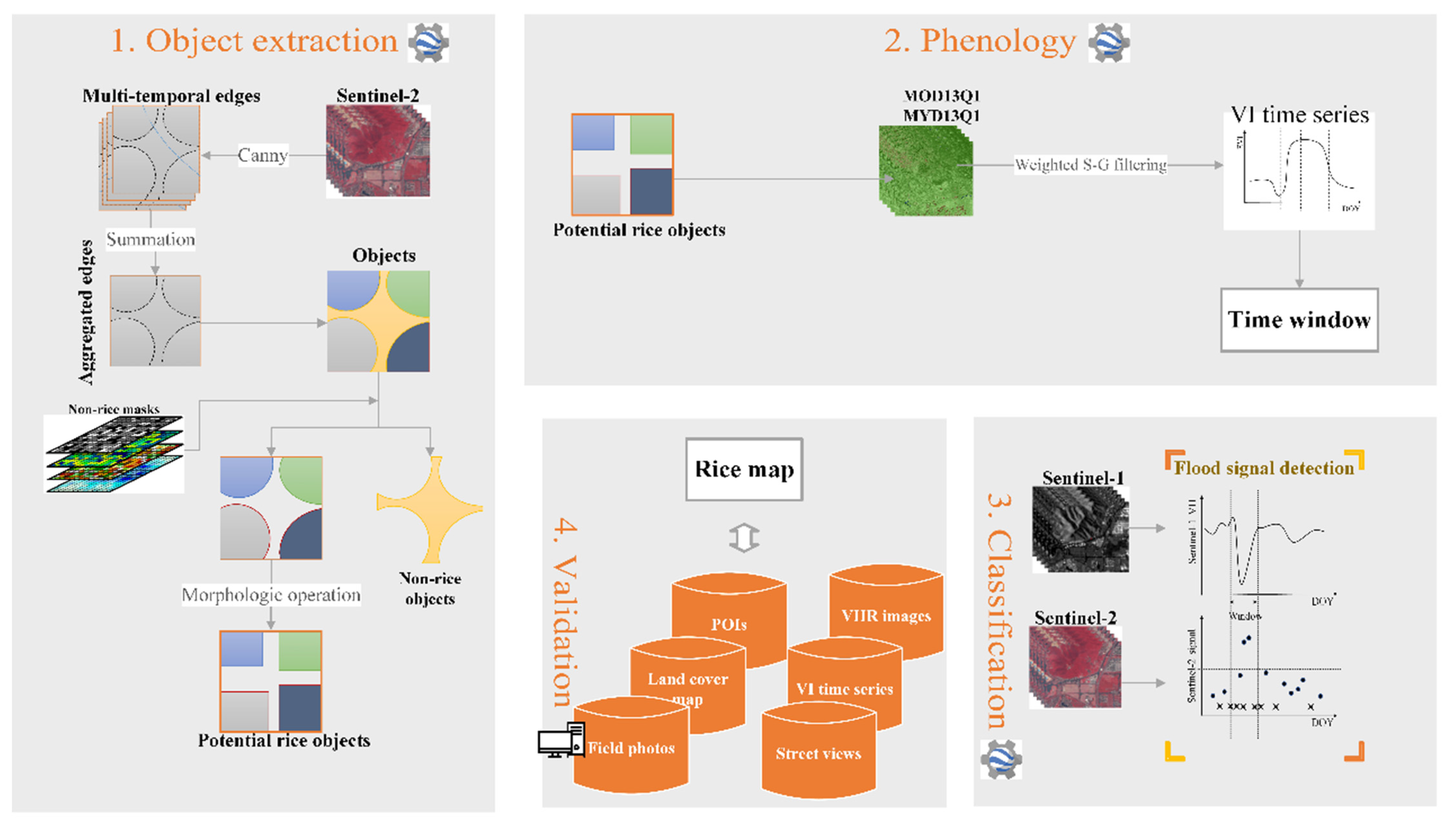
This paper uses the microwave data acquired by Sentinel-1 and the optical data acquired by Sentinel-2 (properties summarized in

Table 1. Sentinel-1/2 data properties.

	Sentinel-1	Sentinel-2
Frequency/Wavelength	5.405 GHz/5.5 cm	-
Polarization/Band	VH	13 spectral bands
Spatial Resolution (m)	10	10, 20, 60
Temporal Resolution (d)	6	5
Incidence Angle	20–47°	-
Mode/Format	IW_GRD	Level-1C
Time Span	1 January 2019 to 1 January 2020

). The Sentinel-1 is the first of the Copernicus Programme satellite constellations launched by the European Space Agency. Its mission is composed of a two-satellite constellation, Sentinel-1A and Sentinel-1B, which share the same orbital plane. They carry C-band SAR instrumentation to provide a collection of all-weather data both day and night. They operate in four acquisition modes: interferometric wide-swath (IW), strip map, extra wide-swath, and wave. The IW is the default acquisition mode over land. The Sentinel-2 is an Earth observation mission from the Copernicus Programme that systematically acquires optical imagery at high spatial resolutions (10–60 m) over land and coastal waters. The mission is a twin-satellite constellation, Sentinel-2A and Sentinel-2B, to achieve a revisit time of five days. The orbit is sun-synchronous at a 786-km altitude with 14.3 revolutions per day and a 10:30 a.m. descending node local overpass time. In this study, only VH polarization of the IW ground-range-detected (GRD) Sentinel-1A imagery was used because this is more sensitive to flooding signals than VV polarization [21]. The year of interest was 2019.

The images obtained from the Sentinel-1 in the Google Earth Engine (GEE) were preprocessed using the Sentinel-1 toolbox. The preprocessing steps are: (1) thermal noise removal, (2) radiometric calibration, (3) terrain correction using SRTM 30 or ASTER DEM for areas greater than 60° latitude when the SRTM is unavailable, and (4) final terrain-corrected value conversion to decibels using log scaling [10*log10(x)]. The Sentinel-2 images were atmospherically corrected using the sen2cor program. The three quality assessment (QA) bands present in the Sentinel-2 images were used to indicate the presence of clouds.

The MGRS with 10 km grids were used to split each Level-1C Sentinel-2 tile (100 km × 100 km) into one hundred grids. The cloud-free Sentinel-2 grids with cloudy pixel percentages less than 5% were selected. By splitting the original tile into smaller grids, more observations on the grid basis can be preserved compared with that on the tile basis. For example, one tile with a cloudy pixel percentage of 50% will be discarded in traditional usable image selection, which is in the unit of an image, but there may be several clear grids with cloudy pixel percentages less than 5% in this image. Though selecting observations on a pixel basis can preserve even more observations, voids due to cloud coverage in images will cause trouble for edge detection. The usage of grids is the trade-off between preserving more observations and suitability for edge detection.

The distribution of clear grids counts in 2019 over the study area is shown in Figure 1.

Besides the Sentinel-1/2 datasets, other datasets used in our study include the 250-m 8-day composite vegetation index products (MOD13Q1 [29] and MYD13Q1 [30]) and land cover-type product (MCD12Q1 [31]) as well as auxiliary data for validation, including VHR images from Google Earth, cadastral data, geo-referenced filed photos, points of interest (POIs), and street views. The cadastral data provided by Bureau of Land Management in Jiashan County, containing information such as plot boundaries, land use type and ownership, is used to validate segmentation and classification. Field photos were acquired from the crowd-sourced field photo library of the University of Oklahoma (http://www.eomf.ou.edu/photos/ (accessed on 1 March 2021)), and the street views and paddy fields related POIs were collected from the Baidu Map (https://map.baidu.com/ (accessed on 1 March 2021)).

3. Methodology

The PODS algorithm includes four modules (see Figure 2) defined as:

• Extract objects from multi-temporal 10-m Sentinel-2 images. The objects are the units used for classification.
• Estimate the time window from the time-series vegetation indices using the PhenoRice algorithm. The time window will be used for classification.
• Object-based flood signal detection using Sentinel-1/2, using objects and time window generated in modules 1 and 2.
• Validation of generated rice map.

The following subsections expand each of these modules.

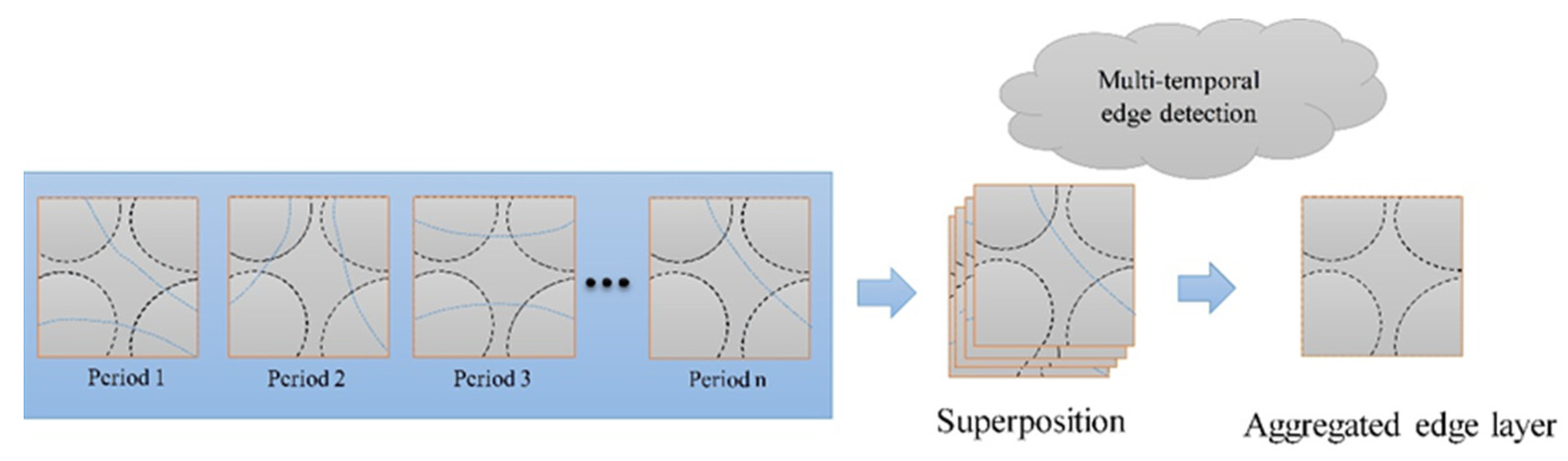
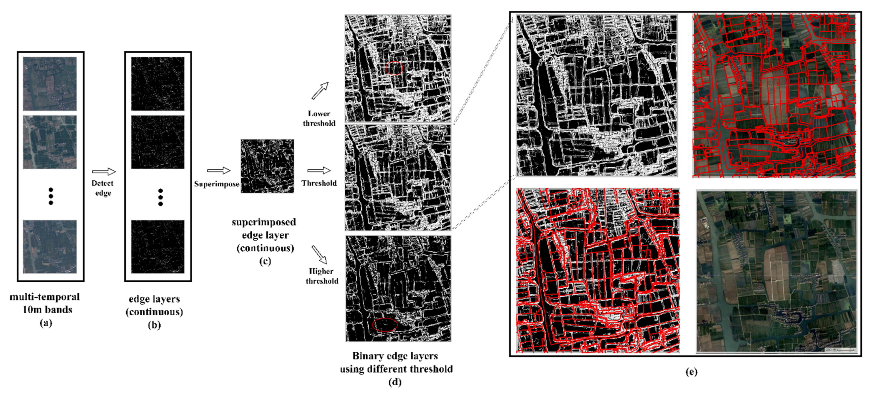
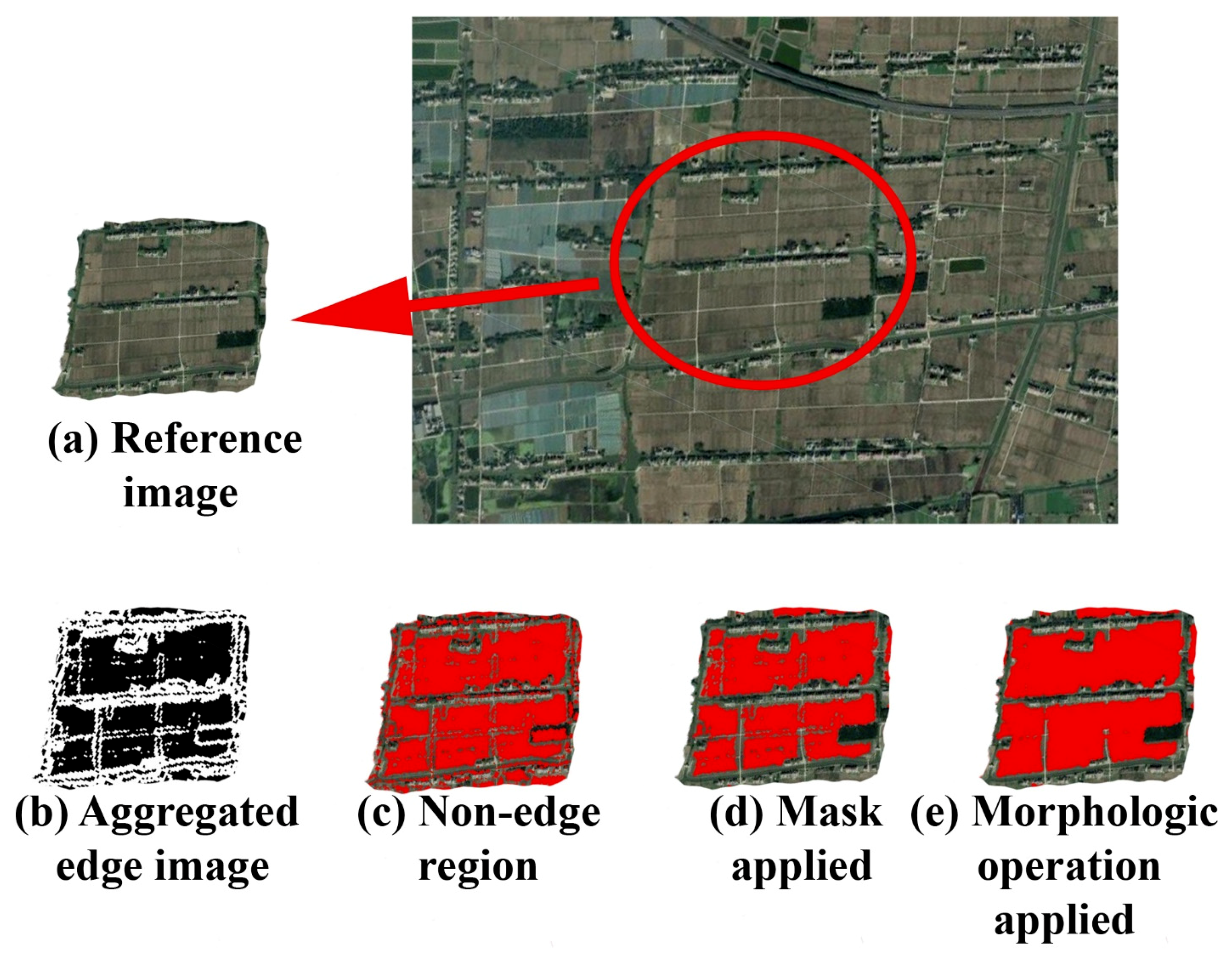
3.1. Object Extraction

Pixel-based classification is commonly adopted when moderate-to-coarse resolution data is used but rarely adopted when finer resolution data is used due to the salt-and-pepper effect resulting from increased pixel heterogeneity. To alleviate such effect, super-pixel or object-based classification can be adopted [32,33,34,35], in which basic classification units approximate parcels or fields.

Finding edges of a field using single-date imagery is challenging when different crop types have similar spectral and structural properties at certain stages of their phenological growth cycle. This challenge is compounded when a single crop is grown on adjacent fields. Therefore, it is necessary to use multiple images throughout the year to accurately detect spatial transitions (edges) between different crop types as well as crops of the same type. Edges in imagery can be defined as a sharp change or discontinuity in the gray-scale values. Various edge detectors have been proposed, such as Sobel, Prewitt, Robert, Scharr, and Canny, to generate the edge layer, which can be described as a gray-scale image that represents object edges. High gray values indicate a sharp discontinuity with adjacent pixels. The Canny operator was used in this study due to its superior performance compared with other edge detection algorithms [24]. We applied the Canny edge operator to image grids from Section 2.2 to extract the edge layers (Figure 3).

Single edge layers have false edges as caused by noise and true edges from fields. A simple equal weight summation of the edge layers was used to combine the images into single, composite, multi-temporal edge images where false edges were faded and true edges were strengthened (Figure 3). The aggregate gradient edge images were divided into edge pixels and non-edge pixels using a threshold. Edge pixels have greater values than the threshold while non-edge pixels have lesser values. As the number of images used in each grid varies (see Figure 1), the thresholds for each grid can change. Generally, a greater number of superimposed images gives a higher threshold. The threshold is set as the product of the image count and a factor, which is determined from trial-and-error experiments. An appropriate factor should keep the integrity of individual plots (assuming the plot grows the same crop) while dividing different plots. A higher (lower) factor causes over- (under)-segmentation. Figure 4 showcases the procedure of multi-temporal edge detection analysis. The edge layer for each date (Figure 4 column b) is the equal-weight aggregation of four edge layers generated from the red, green, blue, and NIR bands. This example qualitatively illustrates how multi-temporal composites of edge layers capture and accentuate persistent field boundaries. Some faint field boundaries (low intensities) on specific dates become more pronounced as images from various dates are combined.

Edge pixels are excluded from subsequent operations and non-edge pixels are retained. These non-edge pixels come from different classes, such as forests, wetlands, built-up areas, and cropland.

Although flooding signals in paddy rice transplanting periods give unique characteristics for paddy rice, flooding signals from other land cover types could also exist during the paddy rice transplanting phase, which mainly includes water bodies (e.g., rivers and lakes) and natural wetlands. In addition, some noise could be caused by miscellaneous non-cropland covers, such as natural vegetation and built-up lands due to some unexpected weather effects. The generation of these non-cropland masks helps reduce sporadic commission errors in the resultant paddy rice maps [11]. We generated several masks by refining the rules used in a previous study [11]. These masks, including sparse and natural vegetation masks, forest masks, as well as slope land masks, were all excluded to minimize commission errors—for example, pixels whose annual maximum vegetation index value is less than 0.3 can be considered as sparse vegetation. Forest and slope land mask are generated from the Japan Aerospace Exploration Agency forest map [22] and Shuttle Radar Topography Mission (SRTM) elevation map [23], respectively.

The unmasked non-edge pixels were clustered into objects based on the four-neighbor connectedness rule. The morphologic operation of closing was then performed to fill holes and smooth boundaries using a 3 × 3 pixel crossing kernel. Figure 5 shows how the workflow is applied to extract objects in a case site.

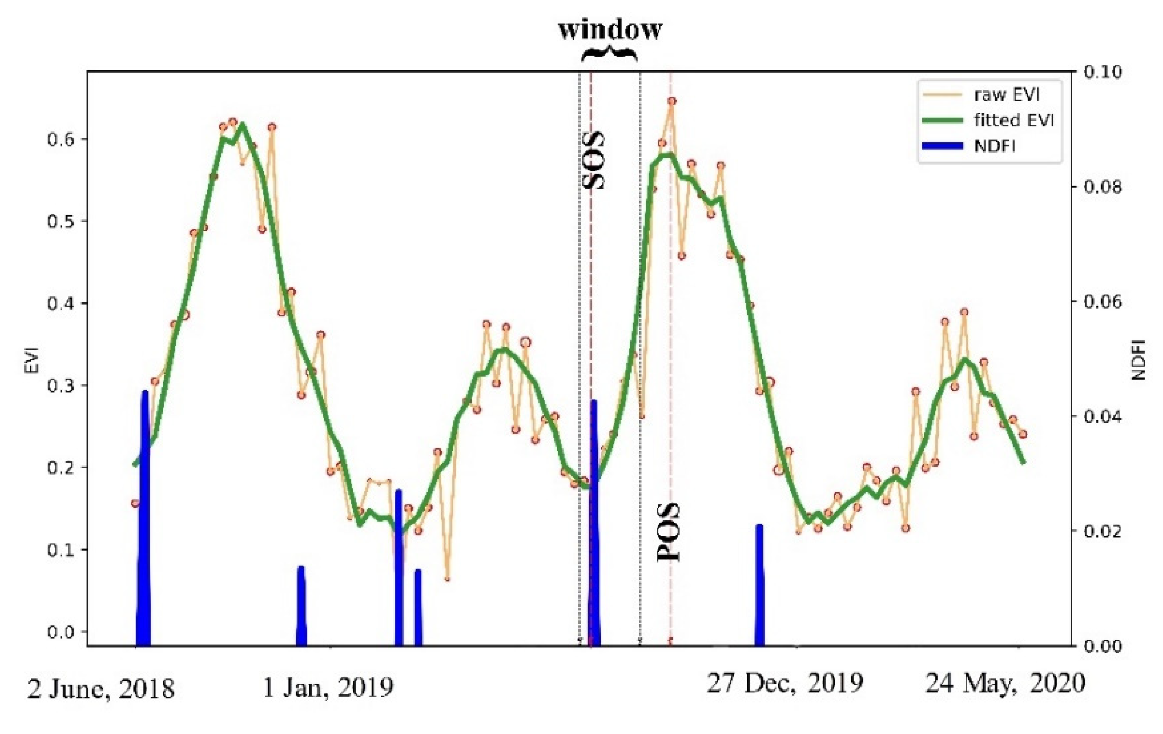
3.2. Time Window Retrieval

When to establish rice depends on genetic, environmental, and management factors [19]. Environment related factors (e.g., temperature [11]) can be used to retrieve rice phenology only if they are the primary limitation for rice planting, which is not the case in the HJH plain. Several researchers used the crop calendar provided by meteorological stations or agricultural observation stations [24,25]. However, these approaches may fail in undeveloped countries where stations are not available and the local agricultural ministry cannot provide a reliable crop calendar. Remote sensing data provide reliable and robust solutions to rice phenology retrieval [26,27,28].

The PhenoRice algorithm monitors information of primarily paddy rice areas, dates for the establishment (Start Of Season, SOS) and flowering (Peak of Season, POS) periods, and cropping intensity by analyzing the time series of individual pixels [19]. For each MODIS pixel (except those excluded by the mask), PhenoRice determines if there is a high probability of belonging to a rice area, estimating the rice crop establishment dates. The EVI time series of each pixel is smoothed using the Savitzky–Golay two-iteration method to reduce noise from cloud contamination or various acquisition angles. The smoothing method assigns weights to the EVI values based on the estimated data quality [13] using information contained in the Pixel Reliability, Usefulness Index, and blue reflectance. The resulting smoothed time series is adapted to the upper envelope of the original curve because those noises have negative biases on original values generally. The smoothed EVI signal is analyzed to identify all local minima and maxima within the time series. Following Manfron et al. [10], these minima and maxima are analyzed based on agronomic criteria (e.g., occurrence of flood event in transplanting phase, the duration from SOS to POS) to determine the presence of a “rice-cycle signal” in the time series. Pixels that meet these criteria are labeled as rice, and their rice crop establishment and flowering dates are estimated. A more detailed description of the PhenoRice algorithm and its performance can be found in [19]. The EVI [29] and normalized flood index (NDFI) used in PhenoRice [19] are calculated as:

$$\mathrm{EVI}=2.5\times \frac{{\rho }_{NIR}-{\rho }_{Red}}{{\rho }_{NIR}+6\times {\rho }_{Red}-7.5\times {\rho }_{Blue}+1}$$

(1)

$$\mathrm{NDFI}=\frac{{\rho }_{Red}-{\rho }_{SWIR}}{{\rho }_{Red}+{\rho }_{SWIR}}$$

(2)

For the exemplar plot (latitude: 30.644440° N, longitude: 120.804088° E), the SOS date determined with the PhenoRice algorithm is the 46th observation in the required time series.

Figure 6 shows the exemplar plots of the PhenoRice estimates for the rice phenological dates (SOS and POS are inflection points in the fitted EVI curve, shown as the orange dotted lines) based on the temporal patterns of the NDFI and the smoothed/raw EVI for different cropping systems for a case pixel. According to temporal profiles of indices over random pixels and local knowledge on cultivation practice, the time window for the flood signal detection is set as the period that starts 10 days before the SOS and ends 50 days after it. It is noted that, as a 250-m pixel often contains a variety of crops, its SOS is determined by the dominant crop type. For example, the SOS of a pixel consisting of 10% rice and 90% forest is the forest SOS (around March) instead of rice (around May). If the time window generated by the forest SOS is used, the number of flood signals detected using the methods in Section 3.3 will be significantly reduced. To ensure the identified SOS is from rice instead of forests (or other crops), the phenology of the non-rice pixels is not estimated. The missing SOS of non-rice pixels is set as the SOS of adjacent rice pixels, assuming that adjacent rice paddies have similar phenology. That is, the SOS of adjacent rice pixels (May) is used as the SOS of the non-rice pixel. Therefore, the SOS for the small number of paddy fields in the exemplar non-rice pixel can be correctly estimated.

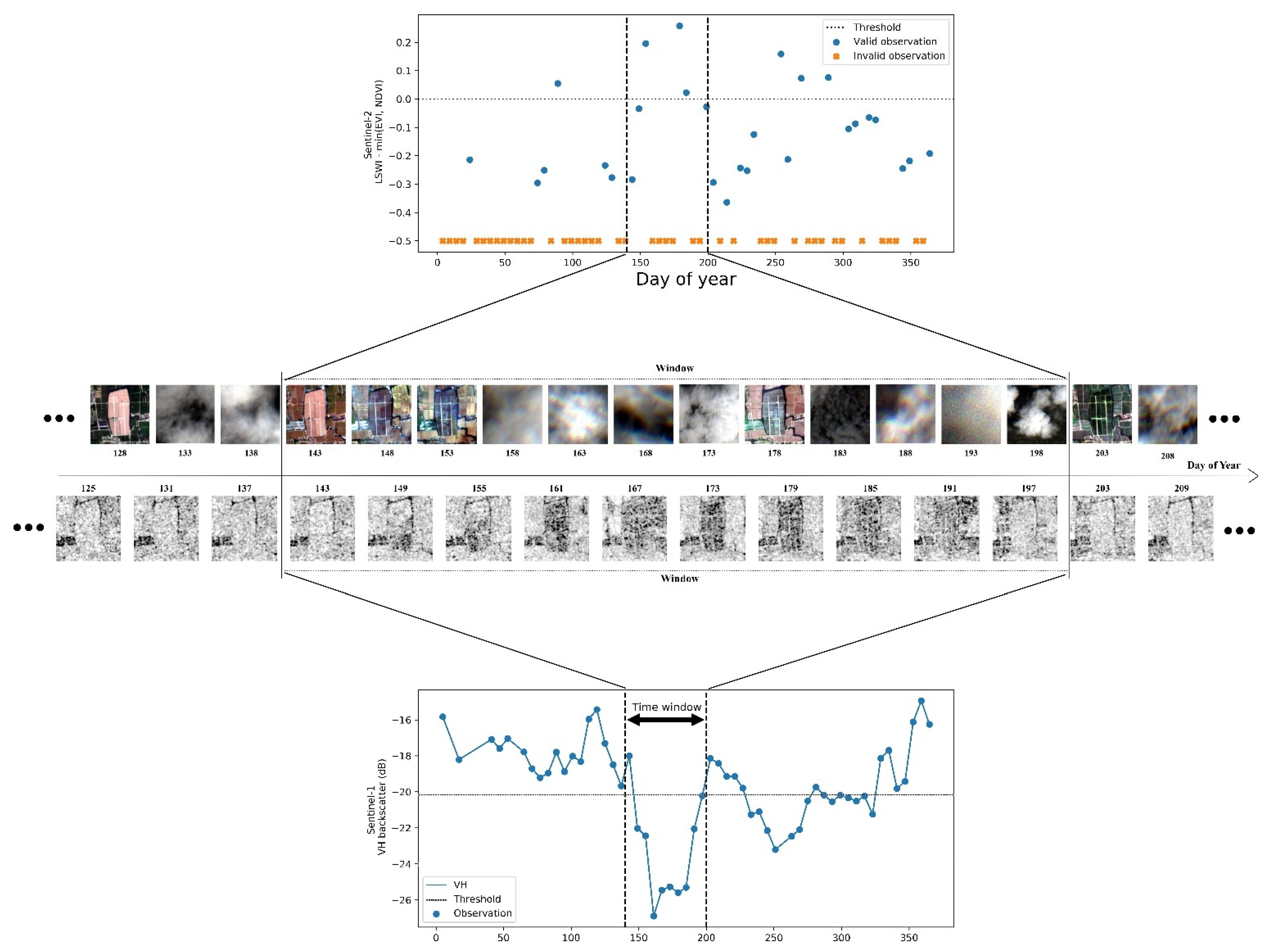
3.3. Flood Signal Detection

Flood signal detection is performed to identify paddy rice for individual objects in their corresponding time windows. The flooding and rice transplanting signals are key features that identify paddy rice fields as this is the only crop that needs to be transplanted in a mixed water–soil environment [30]. The remote sensing recognition of transplanting signals is crucial to identifying paddy rice. Previous studies have revealed that the relationship between the LSWI and NDVI (or EVI) can effectively discriminate flooding/transplanting signals [6]. We performed temporal profile analyses at random paddy rice sites in the study region and found that all the paddy rice agriculture systems in the study area have flooding and transplanting signals in the early growing season that can be captured using vegetation indices. Here, we recognized flooding signals using the LSWI criteria as LSWI-min (EVI, NDVI) > 0. Different from pixel-based classification [11,36], we calculate the signal in the object unit as the mean value of pixels within each object.

Therefore, we detect the flooding and transplanting signals using vegetation indices during the rice transplanting phase. Specifically, the following equation is used [6]:

$$\mathrm{Flood}=\{\begin{array}{ll}1& \mathrm{if} \mathrm{LSW}{\mathrm{I}}_{\mathrm{Ti}}-\min \left({\mathrm{EVI}}_{\mathrm{Ti}},{\mathrm{NDVI}}_{\mathrm{Ti}}\right)>0\\ 0& \mathrm{if} \mathrm{LSW}{\mathrm{I}}_{\mathrm{Ti}}-\min \left({\mathrm{EVI}}_{\mathrm{Ti}},{\mathrm{NDVI}}_{\mathrm{Ti}}\right)\le 0\end{array}(\mathrm{SOT}<T_i<\mathrm{EOT})$$

(3)

where Flood is the status of the flooding/transplanting, and the starting (SOT) and ending (EOT) of the transplanting phase are as defined in Section 3.2, and $T_i$ is the period when the observations are acquired. The spectral indices of NDVI [31], LSWI [7], are calculated using the following equations:

$$\mathrm{NDVI}=\frac{{\rho }_{NIR}-{\rho }_{Red}}{{\rho }_{NIR}+{\rho }_{Red}}$$

(4)

$$\mathrm{LSWI}=\frac{{\rho }_{NIR}-{\rho }_{SWIR}}{{\rho }_{NIR}+{\rho }_{SWIR}}$$

(5)

where ${\rho }_{Blue}$, ${\rho }_{Red}$, ${\rho }_{NIR}$, and ${\rho }_{SWIR}$ are the surface reflectance values of the blue, red, near-infrared, and shortwave-infrared bands from the Sentinel-2 sensor.

SAR data provide complementary observations to optical data, especially in the monsoon season when clouds are prevalent [32,33,34]. The SAR backscattering coefficients for VH polarization over paddy rice fields decrease sharply when flooding occurs but remain relatively stable over non-rice fields throughout the year [35]. A threshold for the backscattering coefficient to divide flood and non-flood areas was successfully applied to SAR data over various frequencies (Henry et al., 2006, Martinis et al., 2015, and Ohki et al., 2016). We selected fifty rice objects and fifty non-rice objects which are evenly distributed over the study area, calculated their minimum VH backscatter intensity during the time window, and applied linear discriminant analysis (LDA) to separate rice and non-rice objects using gamma-naught, which ultimately provides a threshold that separates the two classes [37]. A separation line between two classes can be established and the threshold can be obtained from the LDA with a threshold of −20.1 dB.

Paddy rice can be identified based on its unique flooding characteristics in the transplanting phase. However, variations in transplanting timing for different fields could bias the associated information from one specific image or one image composite [11]. We used a statistics-based approach to delineate the flooding signals by considering all flooding signals during the transplanting phase. The sum of the flooding signals in a given time window for each object (F) is calculated using Equation (6). The threshold for F to identify rice objects is also determined using the LDA approach. Objects whose F value is greater than or equal to 3 are classified as paddy rice.

$$\mathrm{F}={\displaystyle \sum }{\mathrm{Signal}}_{\mathrm{flood}}$$

(6)

Figure 7 shows the time-series optical and microwave signal from the Sentinel-2/1 over an exemplar object (latitude: 30.6444° N, longitude: 120.8041° E). There are ten observations acquired from the Sentinel-1 and twelve from the Sentinel-2 in the specified time window based on the method described in Section 3.2. Six optical observations are obscured by clouds, and four (fourth through the eighth) have positive flood signals because the preceding and following observations (third and ninth) have significant positive flood signals. This is illustrated in the time-series optical signal graph and corresponding images in the first row. Meanwhile, eight of the ten Sentinel-1 observations have positive flood signals with relatively low VH backscatter coefficients. Thus, integrating Sentinel-1 with Sentinel-2 increases the sum of positive flood signals over the object from three to eleven. It is noted that the ninth and twelfth observations from Sentinel-2 in the time window are partially contaminated by clouds, but not flagged in QA bands.

3.4. Validation and Comparison

We used the stratified random sampling approach to acquire validation samples. First, the MODIS land cover products [38] were used to partition the study area into several strata (forest, grassland, wetland, cropland, built-up and barren land, and water body). Second, random points were generated in each stratum, and we made areas of interest (AOIs) as square buffers for the points (100-m × 100-m), as shown in Figure 8b. Third, we checked each AOI with the VHR images and selected and labeled the relatively pure land cover AOIs by referencing both the VHR images from Google Earth and auxiliary information (if any). The AOIs without clear land cover information were excluded. For AOIs with available auxiliary information, such as field photos, street views, or paddy field POIs, the auxiliary information was used to better clarify land cover types. For AOIs without any auxiliary information, the field shape, size, temporal evolution (using Google Earth’s time machine), and vegetation index time series were considered to label the land cover information. Finally, a total of 482 AOIs were generated to validate the resultant paddy rice and non-paddy rice map, including forests (62 AOIs), grasslands (150), wetlands (100), croplands (100), built-up and barren lands (70), and water bodies (50). A confusion matrix for the paddy rice map was calculated to evaluate the accuracy of the results.

Besides the validation, we also compared three pixel-based classification results obtained from three different data sources (Landsat-8, Sentinel-2, and MODIS) along with our object-based results in some randomly selected case regions. The comparison checks the intensity of salt-and-pepper effects that result from data of different spatial resolutions, as well as the advantages of object-based classification over pixel-based approaches to alleviate such effects when moderately high-resolution data are used. For the pixel-based classification, the random forest algorithm [39] available in GEE platform is used, whose number of tree is set as 500 and other parameters as the default. It is often used as a benchmark algorithm because good accuracy could be achieved with a limited number of training samples and default parameter settings [40].

4. Results and Validation

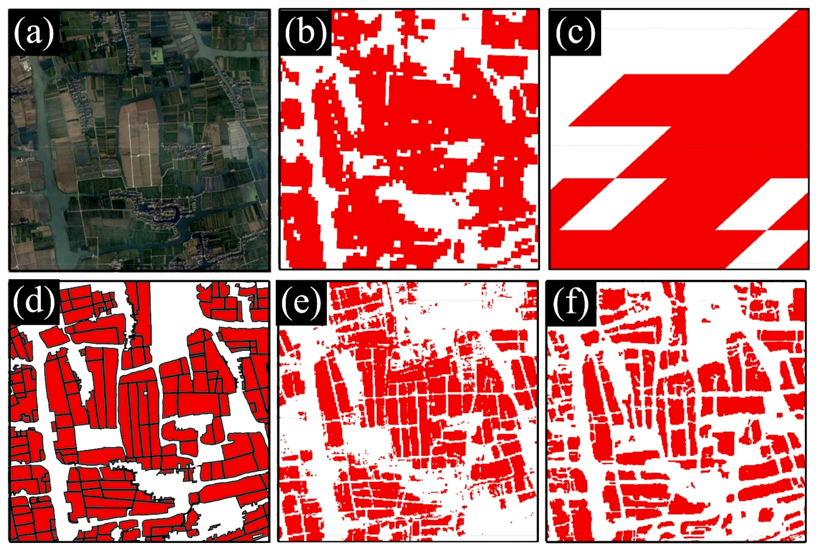
4.1. Field Boundary Delineation

Field boundary delineation has a great impact on further analysis. Two main causes of poor image segmentation are over-segmentation and under-segmentation. The cadastral data provided by land administration in Jiashan County is used as the reference boundary dataset to validate our field boundary delineation. A confusion matrix consisted of 10,000 samples, with 5000 edge samples selected randomly within 10 m of reference boundaries and 5000 non-edge samples randomly selected more than 10 m away from the reference boundaries. Accuracy metrics calculated from the confusion matrix are commission error (CE), omission error (OE), Kappa coefficient, and overall accuracy (OA). The OE indicates how well the extracted edges are in line with reference edge, and a high OE means under-segmentation. The CE measures false edges within fields, and a high OE means over-segmentation. Besides metrics obtained from the confusion matrix, the intersection over union (IoU) score is also used. IoU is a metric to quantify the percentage of overlap between the reference fields and our extracted fields (prediction), which is calculated as:

$$\mathrm{IoU}=\frac{\mathrm{reference}{\displaystyle \cap }\mathrm{prediction}}{\mathrm{reference}{\displaystyle \cup }\mathrm{prediction}}$$

Accuracy metrics in

Table 2. Accuracy metrics for field boundary delineation.

Metric	Value
CE	0.116
OE	0.084
OA	0.898
Kappa	0.796
IoU score	0.718

shows that the field boundary delineation achieves satisfying OA (0.898). The CE and OE are acceptable. Detailed inspections on the prediction results reveal that substantial OEs occur in edges between fields planted with the same crops with similar crop progress, and some CEs are contributed by linear features within the same fields (e.g., irrigation canals and ditches) which are not recorded in cadastral data. As such under-segmentation (the merge of rice fields with similar crop progress) and over-segmentation (caused by irrigation system) will not significantly obscure rice recognition, those fields in reference fields are correspondingly merged and split before calculating IoU score. The IoU score calculated using around four hundred randomly sampled reference fields is 0.718.

4.2. Pattern of Paddy Rice Transplanting Phase

The paddy rice transplanting phase changes over different geographical regions due to various rice genes, environments, and managements. Figure 9 shows the spatial distribution of the SOS.

4.3. Validation and Comparision of Results

Validation based on VHR images, field photos, paddy field POIs, street views, backscatter coefficients, and VI time profiles indicate that the produced paddy rice map in 2019 from the HJH plain had an overall accuracy of 95.4%. The paddy rice category had a producer accuracy (PA) and user accuracy (UA) of 93.7% and 92.6%, respectively. The comparison between three pixel-based paddy rice maps from MODIS, Landsat-8, Sentinel-2, and our PODS-derived paddy rice map showed that all products had a high spatial consistency in the HJH Plain (Figure 10). The Landsat 8-based results had the second highest amount of details, but the Sentinel-2-based results had the most details, excluding roads between paddy rice fields. However, the pixel-based Sentinel-2 rice map suffered from the salt-and-pepper effect across the region, especially in built-up areas, because building shadows were often misclassified as paddy fields due to their spectral similarity, which leads to noteworthy commission errors. Their accuracy assessment metrics are in

Table 3. Accuracy assessment of three pixel-based results from MODIS, Landsat-8 and Sentinel-2, and the object-oriented result generated by PODS.

	MODIS	Landsat	Sentinel-2	PODS
OA	0.869	0.880	0.921	0.954
PA	0.807	0.776	0.907	0.937
UA	0.802	0.850	0.864	0.925
Kappa	0.707	0.724	0.825	0.897
$F_1$	0.805	0.812	0.885	0.931

.

5. Discussion

The phenology- and pixel-based paddy rice mapping algorithm [11] based on flood signal detection is well developed and has been successfully applied to MODIS and Landsat data to produce regional and national rice maps. However, its application to Sentinel-2 data, which has 10-m bands, likely causes a severe salt-and-pepper effect. In addition, algorithms to exploit optical data are not robust when applied to monsoon regions where cloud cover is frequent. The PODS algorithm proposed in our study has three advantages: an object-based classification that uses fields as the basic classification unit to reduce the salt-and-pepper effect; integrating microwave data with optical data to obtain as many positive flood signals as possible in cloudy and rainy regions; and using the PhenoRice algorithm to estimate the transplanting date to address uncertainty in the critical transplanting phase in subtropical/tropical regions. The performance of the PODS algorithm depends on three modules: object extraction, transplanting date estimation, and flood signal detection.

5.1. Object Extraction

Several object-based classification studies use field boundary information obtained from either high-resolution (meter-scale) commercial satellites or local agricultural administrations [41]. However, the cost of commercial data is high and the accessibility of official cadastral data is low. Sentinel-2 satellites, while only having a spatial resolution of 10 m, are not as fine as commercial satellites. However, high temporal resolutions (5–7 d) make up for the limitations of spatial resolution. The fields identified from super-imposed multi-temporal edge layers are promising from our study. The advantage of this approach is that the open and free access to Sentinel-2 data enables scaling of study areas. The past several years have witnessed an increasing number of object-based rice classification researches using Sentinel data [42,43,44]. Among them, the commercial software eCognition [45], providing a number of sophisticated image segmentation algorithms, is often used. However, the fact that it runs on a local computer makes it less suitable to adopt the multi-temporal images approach, since the volume of multi-temporal high-resolution images will overwhelm the PC, especially in the case of a large study region. In contrast, the GEE platform, providing both on-shelf data and computational resources, is more suitable to adopt a multi-temporal images segmentation approach. A multi-temporal image approach solves a primary defect of edge-based image segmentation algorithm, that is, edges between fields can sometimes be weak and false edges within fields may exist in a single image. Besides an edge-based image segmentation approach, there are a few region-based image segmentation approaches on the GEE platform, such as Simple Non-Iterative Clustering (SNIC, [46]). Some researchers have compared edge-based and region-based approaches in recognition of agricultural fields and concluded that the edge-based approach is better because it takes advantage of key characteristics of the agricultural landscape (e.g., ridges or roads surrounding fields) [20].

5.2. Transplanting Phase Determination

MODIS data have been used in several case studies to retrieve rice phenology on a large scale [11,19,47], which has explicitly spatial information and finer resolution than the agricultural phenological calendar released by the agricultural administration, which is usually at the state-level or province-level. In the HJH plain, the 500 m resolution has been able to reflect the general trend of phenology: the difference between distant pixels may be more than 40 days while the difference between adjacent pixels is small. To accommodate potential field variation within the same pixel, a wide time window is adopted at the expense of introducing false signals. Finer resolution of phenological information can narrow the time window, which requires the use of medium resolution satellites, such as Landsat or Sentinel-1/2. Although revisit cycles can be shortened by combining multiple satellites [27]—for example, 5–7 d for Sentinel-2 twins. However, such observation frequency still cannot guarantee a smooth vegetation index time series to be generated, as in the case of exemplar field in Figure 7, where only one valid Sentinel-2 observation is obtained from 153 d to 203 d due to cloud coverage. Cloud coverage is more frequent in a low-latitude area, such as Vietnam, so daily observation frequency is desirable, which could be achieved by image fusion techniques, such as Spatial-Temporal Adaptive Reflectance Fusion Model (STARFM, [48]). Gao [47] used STARFM to fuse MODIS and Landsat data to obtain daily Landsat-like observations, and successfully retrieve plot-level phenology in cloudy areas. However, it is currently not easy to implement this in GEE, so this promising technique is not integrated in our PODS algorithm.

On the other side, SAR backscatter coefficients time series [28] and interferometric coherence time series [49] can be used to retrieve rice phenology, but there are some caveats: SAR data are sensitive to soil moisture (dielectric constant), surface roughness as well as terrain, so non-vegetation factors (e.g., tillage, precipitation) can introduce substantial uncertainty in the time series. Moreover, imaging defects in mountainous regions, such as fore-shortening, shadowing, and overlaying phenomenon, limit its use.

When the region of interest is large, it is necessary to take into consideration all kinds of interfering factors, including terrain, tillage, and precipitation. The vegetation index from optical data is less influenced by these factors and thus is a better proxy of crop progress [50]. Built upon vegetation index time series, the PhenoRice algorithm is reported to be robust and reliable in several case studies [4,51].

5.3. Flood Signal Detection

Following [21], a single global and conservative threshold was used for flood signal detection with microwave data. The influence of the local incidence angle on backscattering hinders the use of a single threshold for the entire scene to a certain extent, but the range of the incident angle of Sentinel-1 is moderate. If the threshold is set higher (lower), the omission error and true positive rates are improved (worsened). Future research will set thresholds as functions of the incidence angle (e.g., piecewise or linear functions) or perform empirical regression-based normalization of the backscatter coefficient to a reference incidence angle [52] by considering the influence of the incidence angle.

The weights of SAR and optical observation in our study are identical, while they could be adjusted depending on terrain, weather, and other conditions. The weight of SAR observation could be reduced when applied to mountainous regions because of the shortages resulted from its acquisition mechanism, such as fore-shortening, overlaying, and shadowing. The sensitivity of backscatter coefficient to soil moisture and ground surface roughness should also be considered.

5.4. Pros and Cons of PODS

The proposed PODS algorithm has the following characteristics, which provide good reproductivity, generality and transferability:

• It was completely implemented on the GEE platform, saving the time of data downloading and taking only several minutes to get the result. Otherwise, it would be computationally unfeasible to implement PODS on general-purpose personal computers because the data volume of Sentinel-1/2 covering the HJH plain, whose area is more than 10 thousand square kilometers, in the whole 2019, is hundreds of gigabytes.
• The datasets used in PODS are those publicly accessible datasets, and neither prior knowledge of the local rice phenology information nor the cadastral field boundary data is required.

The discrimination between rice and non-rice objects is determined by the occurrence of flood signals. However, commission error may occur in those land covers that have flooding phenomenon, such as fish pools and wetlands; omission error may occur in regions where flood signals are weak, e.g., in those regions where upland rice is adopted. Some other distinct characteristics of rice could be incorporated into the current rice classification module to reduce commission and omission error, such as the rapid growth in vegetative phase following the transplanting phase. The rapid growth signal can be captured by a surge in backscatter time series or vegetation index time series [24].

In theory, the PODS algorithm can be applied to regions with different planting intensity and different terrains. However, when applied to different regions, the parameters need to be adjusted. Therefore, this study only selected Hangjiahu Plain as the study area. Double cropping is common in this region, where rice is in rotation with wheat, rapeseed, etc., but double cropping of rice is rare (about 10%). Thus, we didn’t attempt to extract the double cropping rice from the identified rice planting area. The performance assessment of this algorithm in areas with different planting intensity and different terrain will be carried out in the follow-up research.

6. Conclusions

We developed a systematic method to map paddy rice called the PODS algorithm using MODIS and Sentinel-1/2 time series data. The method consists of three procedures: (i) object extraction from multi-temporal 10-m Sentinel-2 data; (ii) specifying the transplanting stage from the time-series VI data using the PhenoRice algorithm; and (iii) identifying rice paddies through flood signal detection from time-series optical and microwave signals (VH backscatter). The PODS algorithm alleviates the pepper-and-salt effect by the object-oriented classification method, accurately recognizes the start of the rice growing season by the PhenoRice method, and solves the low availability of optical remotely sensed images brought by the monsoon climate by optical and radar data fusion. The results were validated against VHR imagery from Google Earth, rice paddy related POIs, geo-referenced field photos, VI time series, and other data sources. The PODS approach is useful when mapping rice paddies in the HJH plain in China. We believe that PODS has potential applicability to other regions where cloud coverage is prevalent, croplands are scattered and fragmented, or the cropping system is complex. In the future, we will test the applicability of this method in a wider range of regions such as south and southeast Asia.

References

1. Kuenzer, C.; Knauer, K. Remote sensing of rice crop areas. Int. J. Remote Sens. 2013, 34, 2101–2139. [Google Scholar] [CrossRef]
2. Jay, M.; Bill, H.; Gene, P.H. Rice Almanac: Source Book for the Most Important Economic Activities on Earth, 4th ed.; IRRI: Los Baños, Philippines, 2013; ISBN 9789712203008. [Google Scholar]
3. Dong, J.; Xiao, X. Evolution of regional to global paddy rice mapping methods: A review. ISPRS J. Photogramm. Remote Sens. 2016, 119, 214–227. [Google Scholar] [CrossRef] [Green Version]
4. Liu, L.; Huang, J.; Xiong, Q.; Zhang, H.; Song, P.; Huang, Y.; Dou, Y.; Wang, X. Optimal MODIS data processing for accurate multi-year paddy rice area mapping in China. GiSci. Remote Sens. 2020, 57, 687–703. [Google Scholar] [CrossRef]
5. Gumma, M.K. Mapping rice areas of South Asia using MODIS multitemporal data. JARS 2011, 5, 53547. [Google Scholar] [CrossRef] [Green Version]
6. Xiao, X.; Boles, S.; Frolking, S.; Salas, W.; Moore, B.; Li, C.; He, L.; Zhao, R. Observation of flooding and rice transplanting of paddy rice fields at the site to landscape scales in China using VEGETATION sensor data. Int. J. Remote Sens. 2002, 23, 3009–3022. [Google Scholar] [CrossRef]
7. Xiao, X.; Boles, S.; Liu, J.; Zhuang, D.; Frolking, S.; Li, C.; Salas, W.; Moore, B. Mapping paddy rice agriculture in southern China using multi-temporal MODIS images. Remote Sens. Environ. 2005, 95, 480–492. [Google Scholar] [CrossRef]
8. Xiao, X.; Boles, S.; Frolking, S.; Li, C.; Babu, J.Y.; Salas, W.; Moore, B. Mapping paddy rice agriculture in South and Southeast Asia using multi-temporal MODIS images. Remote Sens. Environ. 2006, 100, 95–113. [Google Scholar] [CrossRef]
9. Peng, D.; Huete, A.R.; Huang, J.; Wang, F.; Sun, H. Detection and estimation of mixed paddy rice cropping patterns with MODIS data. Int. J. Appl. Earth Obs. Geoinf. 2011, 13, 13–23. [Google Scholar] [CrossRef]
10. Giacinto, M.; Alberto, C.; Mirco, B.; Roberto, C. Testing automatic procedures to map rice area and detect phenological crop information exploiting time series analysis of remote sensed MODIS data. In Remote Sensing for Agriculture, Ecosystems, and Hydrology XIV; International Society for Optics and Photonics: Bellingham, WA, USA, 2012; p. 85311E. [Google Scholar]
11. Dong, J.; Xiao, X.; Menarguez, M.A.; Zhang, G.; Qin, Y.; Thau, D.; Biradar, C.; Moore, B. Mapping paddy rice planting area in northeastern Asia with Landsat 8 images, phenology-based algorithm and Google Earth Engine. Remote Sens. Environ. 2016, 185, 142–154. [Google Scholar] [CrossRef] [Green Version]
12. Wassmann, R.; Jagadish, S.; Heuer, S.; Ismail, A.; Redona, E.; Serraj, R.; Singh, R.K.; Howell, G.; Pathak, H.; Sumfleth, K. Chapter 2 Climate Change Affecting Rice Production: The Physiological and Agronomic Basis for Possible Adaptation Strategies. In Advances in Agronomy; Sparks, D.L., Ed.; Academic Press: Cambridge, MA, USA, 2009; pp. 59–122. ISBN 0065-2113. [Google Scholar]
13. Boschetti, M.; Nelson, A.; Nutini, F.; Manfron, G.; Busetto, L.; Barbieri, M.; Laborte, A.; Raviz, J.; Holecz, F.; Mabalay, M.; et al. Rapid Assessment of Crop Status: An Application of MODIS and SAR Data to Rice Areas in Leyte, Philippines Affected by Typhoon Haiyan. Remote Sens. 2015, 7, 6535–6557. [Google Scholar] [CrossRef] [Green Version]
14. Sakamoto, T.; Yokozawa, M.; Toritani, H.; Shibayama, M.; Ishitsuka, N.; Ohno, H. A crop phenology detection method using time-series MODIS data. Remote Sens. Environ. 2005, 96, 366–374. [Google Scholar] [CrossRef]
15. Sakamoto, T.; van Nguyen, N.; Ohno, H.; Ishitsuka, N.; Yokozawa, M. Spatio–temporal distribution of rice phenology and cropping systems in the Mekong Delta with special reference to the seasonal water flow of the Mekong and Bassac rivers. Remote Sens. Environ. 2006, 100, 1–16. [Google Scholar] [CrossRef]
16. Nguyen, T.T.H.; de Bie, C.A.J.M.; Ali, A.; Smaling, E.M.A.; Chu, T.H. Mapping the irrigated rice cropping patterns of the Mekong delta, Vietnam, through hyper-temporal SPOT NDVI image analysis. Int. J. Remote Sens. 2012, 33, 415–434. [Google Scholar] [CrossRef]
17. Asilo, S.; de Bie, K.; Skidmore, A.; Nelson, A.; Barbieri, M.; Maunahan, A. Complementarity of Two Rice Mapping Approaches: Characterizing Strata Mapped by Hypertemporal MODIS and Rice Paddy Identification Using Multitemporal SAR. Remote Sens. 2014, 6, 12789–12814. [Google Scholar] [CrossRef] [Green Version]
18. Tornos, L.; Huesca, M.; Dominguez, J.A.; Moyano, M.C.; Cicuendez, V.; Recuero, L.; Palacios-Orueta, A. Assessment of MODIS spectral indices for determining rice paddy agricultural practices and hydroperiod. ISPRS J. Photogramm. Remote Sens. 2015, 101, 110–124. [Google Scholar] [CrossRef] [Green Version]
19. Boschetti, M.; Busetto, L.; Manfron, G.; Laborte, A.; Asilo, S.; Pazhanivelan, S.; Nelson, A. PhenoRice: A method for automatic extraction of spatio-temporal information on rice crops using satellite data time series. Remote Sens. Environ. 2017, 194, 347–365. [Google Scholar] [CrossRef] [Green Version]
20. Watkins, B.; van Niekerk, A. A comparison of object-based image analysis approaches for field boundary delineation using multi-temporal Sentinel-2 imagery. Comput. Electron. Agric. 2019, 158, 294–302. [Google Scholar] [CrossRef]
21. Nguyen, D.B.; Gruber, A.; Wagner, W. Mapping rice extent and cropping scheme in the Mekong Delta using Sentinel-1A data. Remote Sens. Lett. 2016, 7, 1209–1218. [Google Scholar] [CrossRef]
22. Shimada, M.; Itoh, T.; Motooka, T.; Watanabe, M.; Shiraishi, T.; Thapa, R.; Lucas, R. New global forest/non-forest maps from ALOS PALSAR data (2007–2010). Remote Sens. Environ. 2014, 155, 13–31. [Google Scholar] [CrossRef]
23. CGIAR-CSI SRTM—SRTM 90 m DEM Digital Elevation Database. Available online: https://srtm.csi.cgiar.org/ (accessed on 28 February 2021).
24. Zhan, P.; Zhu, W.; Li, N. An automated rice mapping method based on flooding signals in synthetic aperture radar time series. Remote Sens. Environ. 2021, 252, 112112. [Google Scholar] [CrossRef]
25. Zhou, Y.; Xiao, X.; Qin, Y.; Dong, J.; Zhang, G.; Kou, W.; Jin, C.; Wang, J.; Li, X. Mapping paddy rice planting area in rice-wetland coexistent areas through analysis of Landsat 8 OLI and MODIS images. Int. J. Appl. Earth Obs. Geoinf. 2016, 46, 1–12. [Google Scholar] [CrossRef] [PubMed] [Green Version]
26. Huang, X.; Liu, J.; Zhu, W.; Atzberger, C.; Liu, Q. The Optimal Threshold and Vegetation Index Time Series for Retrieving Crop Phenology Based on a Modified Dynamic Threshold Method. Remote Sens. 2019, 11, 2725. [Google Scholar] [CrossRef] [Green Version]
27. Boschetti, M.; Busetto, L.; Ranghetti, L.; Haro, J.G.; Campos-Taberner, M.; Confalonieri, R. Testing Multi-Sensors Time Series of Lai Estimates to Monitor Rice Phenology: Preliminary Results. In Proceedings of the 2018 IEEE International Geoscience & Remote Sensing Symposium, Valencia, Spain, 22–27 July 2018; IEEE: Piscataway, NJ, USA, 2018; pp. 8221–8224, ISBN 978-1-5386-7150-4. [Google Scholar]
28. He, Z.; Li, S.; Wang, Y.; Dai, L.; Lin, S. Monitoring Rice Phenology Based on Backscattering Characteristics of Multi-Temporal RADARSAT-2 Datasets. Remote Sens. 2018, 10, 340. [Google Scholar] [CrossRef] [Green Version]
29. Huete, A.; Didan, K.; Miura, T.; Rodriguez, E.; Gao, X.; Ferreira, L. Overview of the radiometric and biophysical performance of the MODIS vegetation indices. Remote Sens. Environ. 2002, 83, 195–213. [Google Scholar] [CrossRef]
30. Le Toan, T.; Ribbes, F.; Wang, L.-F.; Floury, N.; Ding, K.-H.; Kong, J.A.; Fujita, M.; Kurosu, T. Rice crop mapping and monitoring using ERS-1 data based on experiment and modeling results. IEEE Trans. Geosci. Remote Sens. 1997, 35, 41–56. [Google Scholar] [CrossRef]
31. Tucker, C.J. Red and photographic infrared linear combinations for monitoring vegetation. Remote Sens. Environ. 1979, 8, 127–150. [Google Scholar] [CrossRef] [Green Version]
32. Poortinga, A.; Tenneson, K.; Shapiro, A.; Nquyen, Q.; San Aung, K.; Chishtie, F.; Saah, D. Mapping Plantations in Myanmar by Fusing Landsat-8, Sentinel-2 and Sentinel-1 Data along with Systematic Error Quantification. Remote Sens. 2019, 11, 831. [Google Scholar] [CrossRef] [Green Version]
33. Torbick, N.; Salas, W.A.; Hagen, S.; Xiao, X. Monitoring Rice Agriculture in the Sacramento Valley, USA With Multitemporal PALSAR and MODIS Imagery. IEEE J. Sel. Top. Appl. Earth Obs. Remote Sens. 2011, 4, 451–457. [Google Scholar] [CrossRef]
34. Okamoto, K. Estimation of rice-planted area in the tropical zone using a combination of optical and microwave satellite sensor data. Int. J. Remote Sens. 1999, 20, 1045–1048. [Google Scholar] [CrossRef]
35. Veloso, A.; Mermoz, S.; Bouvet, A.; Le Toan, T.; Planells, M.; Dejoux, J.-F.; Ceschia, E. Understanding the temporal behavior of crops using Sentinel-1 and Sentinel-2-like data for agricultural applications. Remote Sens. Environ. 2017, 199, 415–426. [Google Scholar] [CrossRef]
36. Clauss, K.; Ottinger, M.; Kuenzer, C. Mapping rice areas with Sentinel-1 time series and superpixel segmentation. Int. J. Remote Sens. 2018, 39, 1399–1420. [Google Scholar] [CrossRef] [Green Version]
37. Wakabayashi, H.; Motohashi, K.; Kitagami, T.; Tjahjono, B.; Dewayani, S.; Hidayat, D.; Hongo, C. Flooded Area Extraction of Rice Paddy Field in Indonesia Using SENTINEL-1 SAR Data. Int. Arch. Photogramm. Remote Sens. Spat. Inf. Sci. 2019, XLII-3/W7, 73–76. [Google Scholar] [CrossRef] [Green Version]
38. Friedl, D.S.-M. MCD12Q1 MODIS/Terra+Aqua Land Cover Type Yearly L3 Global 500 m SIN Grid V006. 2015. Available online: https://developers.google.com/earth-engine/datasets/catalog/MODIS_006_MCD12Q1?hl=en#citations (accessed on 4 March 2021).
39. Breiman, L. Random Forests. Mach. Learn. 2001, 45, 5–32. [Google Scholar] [CrossRef] [Green Version]
40. Zhang, X.; Wu, B.; Ponce-Campos, G.; Zhang, M.; Chang, S.; Tian, F. Mapping up-to-Date Paddy Rice Extent at 10 M Resolution in China through the Integration of Optical and Synthetic Aperture Radar Images. Remote Sens. 2018, 10, 1200. [Google Scholar] [CrossRef] [Green Version]
41. Lin, M.-L. Mapping paddy rice agriculture in a highly fragmented area using a geographic information system object-based post classification process. JARS 2012, 6, 63526. [Google Scholar] [CrossRef]
42. Belgiu, M.; Csillik, O. Sentinel-2 cropland mapping using pixel-based and object-based time-weighted dynamic time warping analysis. Remote Sens. Environ. 2018, 204, 509–523. [Google Scholar] [CrossRef]
43. Rudiyanto; Minasny, B.; Shah, R.M.; Che Soh, N.; Arif, C.; Indra Setiawan, B. Automated Near-Real-Time Mapping and Monitoring of Rice Extent, Cropping Patterns, and Growth Stages in Southeast Asia Using Sentinel-1 Time Series on a Google Earth Engine Platform. Remote Sens. 2019, 11, 1666. [Google Scholar] [CrossRef] [Green Version]
44. Lasko, K.; Vadrevu, K.P.; Tran, V.T.; Justice, C. Mapping Double and Single Crop Paddy Rice With Sentinel-1A at Varying Spatial Scales and Polarizations in Hanoi, Vietnam. IEEE J. Sel. Top. Appl. Earth Obs. Remote Sens. 2018, 11, 498–512. [Google Scholar] [CrossRef]
45. eCognition|Trimble Geospatial. Available online: https://geospatial.trimble.com/products-and-solutions/ecognition (accessed on 6 February 2021).
46. Achanta, R.; Süsstrunk, S. Superpixels and Polygons Using Simple Non-iterative Clustering. In Proceedings of the 2017 IEEE Conference on Computer Vision and Pattern Recognition (CVPR), Honolulu, HI, USA, 21–26 July 2017; pp. 4895–4904, ISBN 1063-6919. [Google Scholar]
47. Gao, F.; Anderson, M.C.; Zhang, X.; Yang, Z.; Alfieri, J.G.; Kustas, W.P.; Mueller, R.; Johnson, D.M.; Prueger, J.H. Toward mapping crop progress at field scales through fusion of Landsat and MODIS imagery. Remote Sens. Environ. 2017, 188, 9–25. [Google Scholar] [CrossRef] [Green Version]
48. Gao, F.; Masek, J.; Schwaller, M.; Hall, F. On the blending of the Landsat and MODIS surface reflectance: Predicting daily Landsat surface reflectance. IEEE Trans. Geosci. Remote Sens. 2006, 44, 2207–2218. [Google Scholar] [CrossRef]
49. Shang, J.; Liu, J.; Poncos, V.; Geng, X.; Qian, B.; Chen, Q.; Dong, T.; Macdonald, D.; Martin, T.; Kovacs, J.; et al. Detection of Crop Seeding and Harvest through Analysis of Time-Series Sentinel-1 Interferometric SAR Data. Remote Sens. 2020, 12, 1551. [Google Scholar] [CrossRef]
50. You, X.; Meng, J.; Zhang, M.; Dong, T. Remote Sensing Based Detection of Crop Phenology for Agricultural Zones in China Using a New Threshold Method. Remote Sens. 2013, 5, 3190–3211. [Google Scholar] [CrossRef] [Green Version]
51. Busetto, L.; Zwart, S.J.; Boschetti, M. Analysing spatial–temporal changes in rice cultivation practices in the Senegal River Valley using MODIS time-series and the PhenoRice algorithm. Int. J. Appl. Earth Obs. Geoinf. 2019, 75, 15–28. [Google Scholar] [CrossRef]
52. Nguyen, D.; Wagner, W.; Naeimi, V.; Cao, S. Rice-planted area extraction by time series analysis of ENVISAT ASAR WS data using a phenology-based classification approach: A case study for Red River Delta, Vietnam. In ISPRS—International Archives of the Photogrammetry, Remote Sensing and Spatial Information Sciences, Proceedings of the 36th International Symposium on Remote Sensing of Environment (Volume XL-7/W3), Berlin, Germany, 11–15 May 2015; Copernicus GmbH: Göttingen, Germany, 2015; pp. 77–83. ISBN 1682-1750. [Google Scholar]
Figure 1. The lower-left map indicates the location of the study area in a coordinate reference system of WGS 84 UTM zone 51, overlaid with the Military Grid Reference System (MGRS) 10-km grids, the colors of which indicate the number of clear images with cloud pixel percentage less than 5% from Sentinel-2 in 2019.
Remotesensing 13 00990 g001
Figure 2. Schematic diagram of the processing chain for the proposed algorithm. The first three modules are implemented in GEE while the fourth module, validation, is implemented on a local computer.
Remotesensing 13 00990 g002
Figure 3. Edge detection based on multi-temporal images where the blue lines denote false edges and black dashed lines denote true edges.
Remotesensing 13 00990 g003
Figure 4. The workflow graph showcases the procedure of multi-temporal edge detection analysis. Multiple edge layers (b) are extracted from multiple corresponding Sentinel-2 10m bands (a), then superimposed to single edge layer (c). The continuous edge layer is thresholded to binary edge layers (d), where the black is non-edge region (agricultural fields) and the white is the edge region. The red ellipses in (d) show examples of over-segmentation where a single field is separated by false edges, and under-segmentation where multiple fields with different crops planted are not separated. (e) from left to right and top to bottom shows the zoom-in binary edge of that in the middle of (d), reference edge over VHR images, reference edge over detected edge, and VHR image, respectively. It should be noted that we use cadastral boundaries as reference edges, so some reference edges are redundant (e.g., division lines in river) and some are missing where multiple fields have the same ownership.
Remotesensing 13 00990 g004
Figure 5. Illustration of the object extraction process.
Remotesensing 13 00990 g005
Figure 6. The NDFI, raw and fitted EVI are in blue, orange, and green, respectively. The size of the red cycle (big/medium/small) denotes the quality of the associated observation (great/good/bad).
Remotesensing 13 00990 g006
Figure 7. Top and bottom panels show the time profiles for the optical and microwave signals over an exemplar object, respectively. In the top panel, blue dots denote valid observation (not flagged as cloud or cloud shadow in QA bands) while orange crosses denote invalid observation (flagged as cloud or cloud shadow). In the bottom panel, all observations are valid because SAR data are independent from weather and illumination conditions, thus they marked as blue dots. The corresponding observation images in the time profile are given in the middle two rows, displayed in true colors for Sentinel-2 and a grey image for Sentinel-1 VH.
Remotesensing 13 00990 g007
Figure 8. (a) is the distribution of stratified samples for points from the MCD12Q1 land cover map, farm POIs, and field photos; (b) is an example of a square AOI for one sample; (c) is an example of geo-referenced field photo acquired from (d) the site (http://www.eomf.ou.edu/photos/ (accessed on 1 March 2021)).
Remotesensing 13 00990 g008
Figure 9. Pattern of the start of the season.
Remotesensing 13 00990 g009
Figure 10. Comparison between three pixel-based classification results from MODIS, Landsat, and Sentinel-2 along with our results derived from PODS. The red is rice fields. (a) VHR reference image from Google Earth Engine, (b) 30-m Landsat 8 pixel-based result, (c) 250-m MODIS pixel-based result, (d) the reference rice fields, surrounded by cadastral boundaries (black), (e) 10-m Sentinel-2 pixel-based result, and (f) PODS object-oriented result.
Remotesensing 13 00990 g010