1. Introduction
Maritime vessel detection from waterborne images is a crucial aspect in various fields involving maritime traffic supervision and management, marine surveillance and navigation safety. Prevailing ship detection techniques exploit either remote sensing images or radar images, which can hinder the performance of real-time applications [
1]. Satellites can provide near real-time information, but satellite image acquisition, however, can be unpredictable, since it is challenging to determine which satellite sensors can provide the relevant imagery in a narrow collection window [
2]. Hence, seaborne visual imagery can tremendously help in essential tasks both in civilian and military applications, since it can be collected in real-time from surveillance videos, for instance.
Ship detection in a traditional setting depends extensively on human monitoring, which is highly expensive and unproductive. Moreover, the complexity of the maritime environment makes it difficult for humans to focus on video footage for prolonged periods of time [
3]. Machine vision, however, can take the strain from human resources and provide solutions for ship detection. Traditional methods based on feature extraction and image classification, involving background subtraction and foreground detection, as well as directional gradient histograms, are highly affected by datasets exhibiting challenging environmental factors (glare, fog, clouds, high waves, rain etc.), background noise or lighting conditions.
Convolutional neural networks (CNNs) contributed massively to the image classification and object detection tasks in the past years [
4,
5,
6,
7,
8]. They incorporate feature extractors and classifiers in multilayer architectures, whose number of layers regulate their selectiveness and feature invariance. CNNs exploit convolutional and pooling layers extracting local features, and gradually advancing object representation from simple features to complex structures, across multiple layers. CNN-based detectors can subtract compelling distinguishable features automatically unlike more traditional methods which use predefined features, manually selected. However, integrating ship features into detection proves to be challenging even in this context, given the complexity of environmental factors, object occlusion, ship size variation, occupied pixel area etc. This often leads to unsatisfactory performance of detectors on ship datasets.
To address ship detection in a range of operating scenarios, including various atmospheric conditions, background variations and illumination, we introduce a new dataset consisting of 9880 images, and annotations comprising carefully annotated objects.
The paper is organized as follows.
Section 2 describes related work, including notable results in vessel detection and maritime datasets comprising waterborne images.
Section 3 describes data acquisition, dataset diversity, dataset design and our relabelling algorithm along with basic dataset statistics based on the final annotation data. In
Section 4, we discuss evaluation criteria and present experimental results; we investigate four CNN-based detectors and discuss the feature extractors and object size effect on the performance of the detectors.
Section 5 provides a qualitative overview of the experimental results. In
Section 6, we provide a brief analysis of our dataset specifications in comparison with other similar datasets. Conclusions are presented in
Section 7.
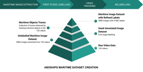
3. Materials and Methods
3.1. Camera System
The dataset was acquired from a set of 135 videos, collected from a sightseeing watercraft, by a camera with a field of view of and stored in FullHD (1920 × 720) resolution at 15 FPS in MPEG format. The route of the watercraft extended from the city of Turku to Ruissalo in South-West Finland, the videos comprising the urban area along the Aura river, the port and the Finnish Archipelago, for a duration of 13 days (26 June 2018–8 July 2018). The watercraft ran each day in a timeframe between 10.15 and 16.45. The videos were captured into 30-min long periods consisting of footage from the route that the watercraft took. While the route remained largely the same, the data contains a variety of typical maritime scenarios in a range of weather conditions.
In addition to camera video data, the platform had a LiDAR attached to it (SICK LD-MRS, FoV 110 degrees, 2 × 4 planes, up to 300 m detection, at 5 Hz). The data from the LiDAR was captured alongside the video at a rate of 5 entries of up to 800 points per s. Given the utilized LiDAR had a detection range of up to 300 m, it was very useful for detecting other objects in the harbor environment. Due to having only 2 times 4 lasers in the height direction however, the provided data was not reliable enough for discerning the nature of the object (i.e., what object was detected). It was useful however to determine distances to the objects perceived in the videos. For the purpose of creating the dataset presented in this paper, we used the LiDAR data to filter out video segments that were captured in the harbor area (usually the ones that had too many points for a prolonged period of time).
To evaluate the models, we acquired 9880 image photos from the videos. First, we annotated all images with 11 categories: seamarks, 9 types of maritime vessels, and miscellaneous floaters. In a second round, we relabelled all the inconsistencies we found, using an algorithm based on the CSRT tracker [
20].
3.2. Dataset Diversity
Maritime environments are inherently intricate, hence a range of factors have to be accounted for when desinging a dataset. Dataset design must ensure that the dataset characterizes well vessels in the environment. Of course, data augmentation methods can be considered for reproducing certain environmental conditions, however authentic conditions may be difficult to anticipate.
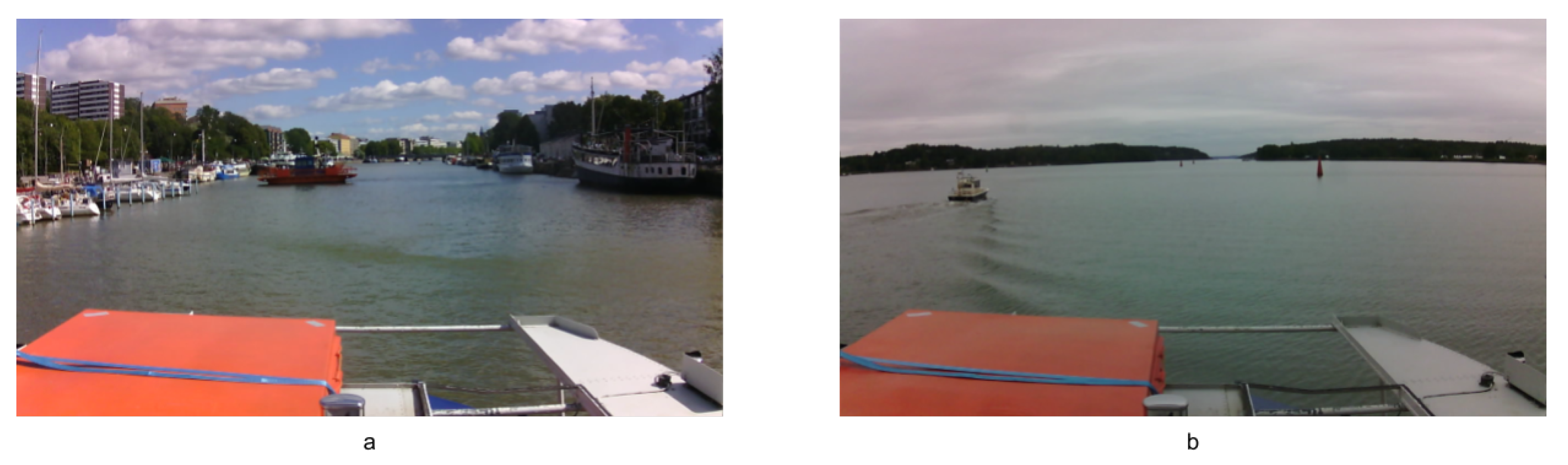
Background variation. Particular object detection tasks are more prone to be affected by changes in the background of the picture. For instance, facial recognition is less susceptible to background variations, because given the similar shape of most faces, it is easier to fit them into bounding boxes in a congruous manner. However, the shapes of maritime vessels are highly heterogeneous, making them more difficult to separate from the background due to a potentially vast background information in the bounding box. The accuracy of ship detection would be significantly affected if background information were classified as ship features.
Figure 1 illustrates the background variation of images in our datasets, including urban landscapes and an open sea environment.
Atmospheric conditions. Atmospheric conditions were specific to Finnish summers, with very sunny periods, alternating with rainy intervals and cloudy skies. The dataset includes a variety of images of different atmospheric conditions throughout a day.
Illumination. Lighting variations can significantly impact image capture. Illumination throughout the day, in various geographical areas and with specific daylight hours in a given region can dramatically influence image detection.
Visible proportion. A great number of the images in our dataset consists of moving ships, with objects being only partially captured in the camera field of view. However, they still represent objects that were annotated since one has to detect them as well. The annotation should comprise different visible proportions of the maritime vessels.
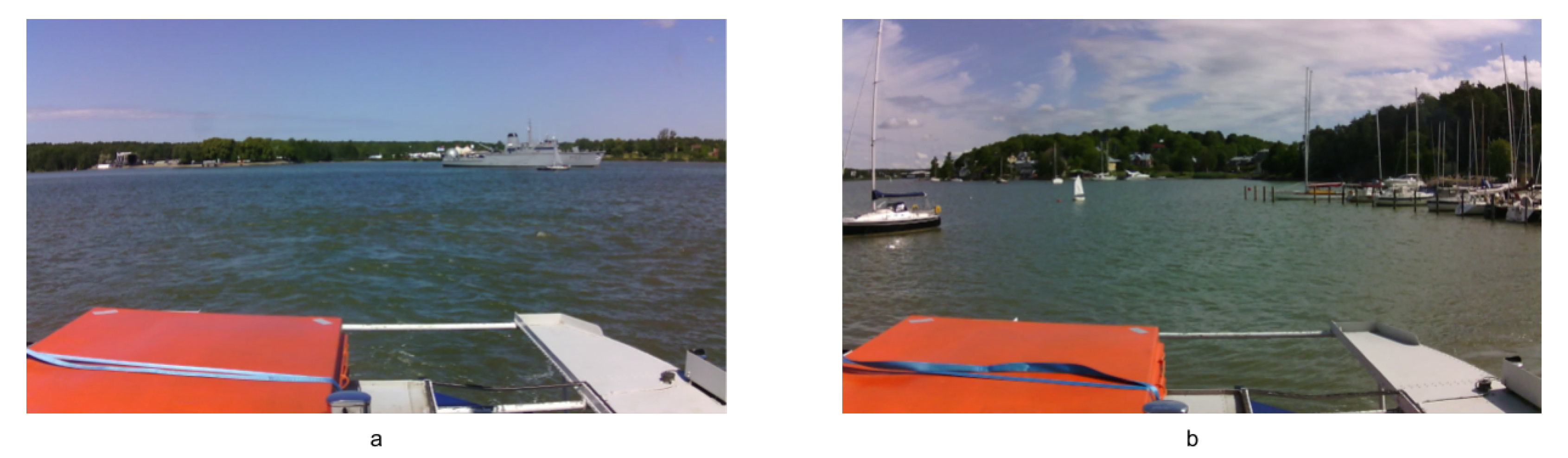
Occlusion. Due to the fact that our dataset has been captured in an open sea environment, in the harbor area and also comprises urban landscapes, there are many occasions when maritime vessels occlude each other or occlude other objects in the environment in the harbor area or in the urban landscape. In a subset of pictures especially in the harbor area, there is significant occlusion due to a high number of maritime vessels in the proximity of each other. Two examples of occlusion are shown in
Figure 2.
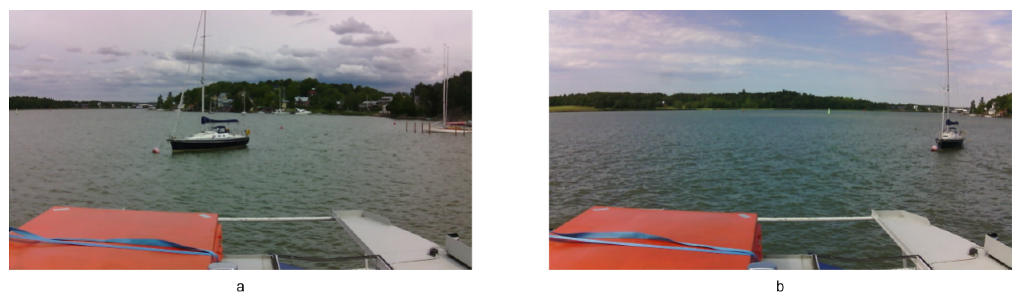
Scale variation. Detection of small object can prove to be quite difficult, especially in a complex environment like the sea, ships that occupy a small pixel area in the picture can be confused with other objects in the background. Maintaining a high level of detection for ships requires including several scales for ships sizes in the dataset. For more information regarding the annotation and the size of the bounding boxes, please refer to
Section 3.4.
Figure 3 illustrates a sailboat from two different perspectives: a lateral and a frontal view, which shows a variation in both occupied pixel area, but also the visible proportion.
3.3. Dataset Design
The raw data acquired from the camera on the sightseeing watercraft is captured as MPEG videos, with 720 p resolution at 15 FPS. The videos include some footage exhibiting content that is irrelevant for the scope of vessel detection (especially footage captured when the watercraft was docked, either at the start of its route on the Aura river or at the Port of Turku) or sensitive content, such as faces of people. To address the latter issue, we performed face detection on all videos and blurred all detected faces. Addressing the former issue on the other hand, required additional data from the LiDAR.
In a maritime environment, LiDAR data is relatively sparse, authors of this study observed that a high number of points detected for a prolonged duration correlates with the watercraft being docked in the harbor. By setting a point threshold to detect these (docked/harbor) cases, we were able to filter them out in their majority and extract only the images regarding mostly the maritime environment. The images were extracted at an interval of 15 s (one image every 225 frames) and still contained some images captured during docking, but most of them were facing outwards from the harbor, so the images captured in this manner still contain useful maritime data. As a result we acquired 9880 images in the maritime environment.
The acquired images were subsequently separated into workpackages in such a manner that chronologically adjacent pictures were separated into different workpackages. The workpackages were then manually labelled by different annotators. After the initial labelling was completed, we used the CSRT tracker [
20] to combine labels of the same object into traces, i.e., a collection of chronologically adjacent images containing a bounding-box for that object. Due to inaccuracies in the tracking process and discrepancies in labelling, the produced traces were not always accurate. After viewing the labels in these traces, we identified the main causes for discrepancies in labelling, which were mainly caused by different interpretations of label annotations. We refined those annotations to eliminate the discrepancies and separated the data into a second collection of workpackages that were provided to annotators, who then relabelled the data, according to refined annotations. After the relabelling was completed, the images and their refined labels were compiled into a dataset of maritime images with refined annotations.
3.4. Annotation
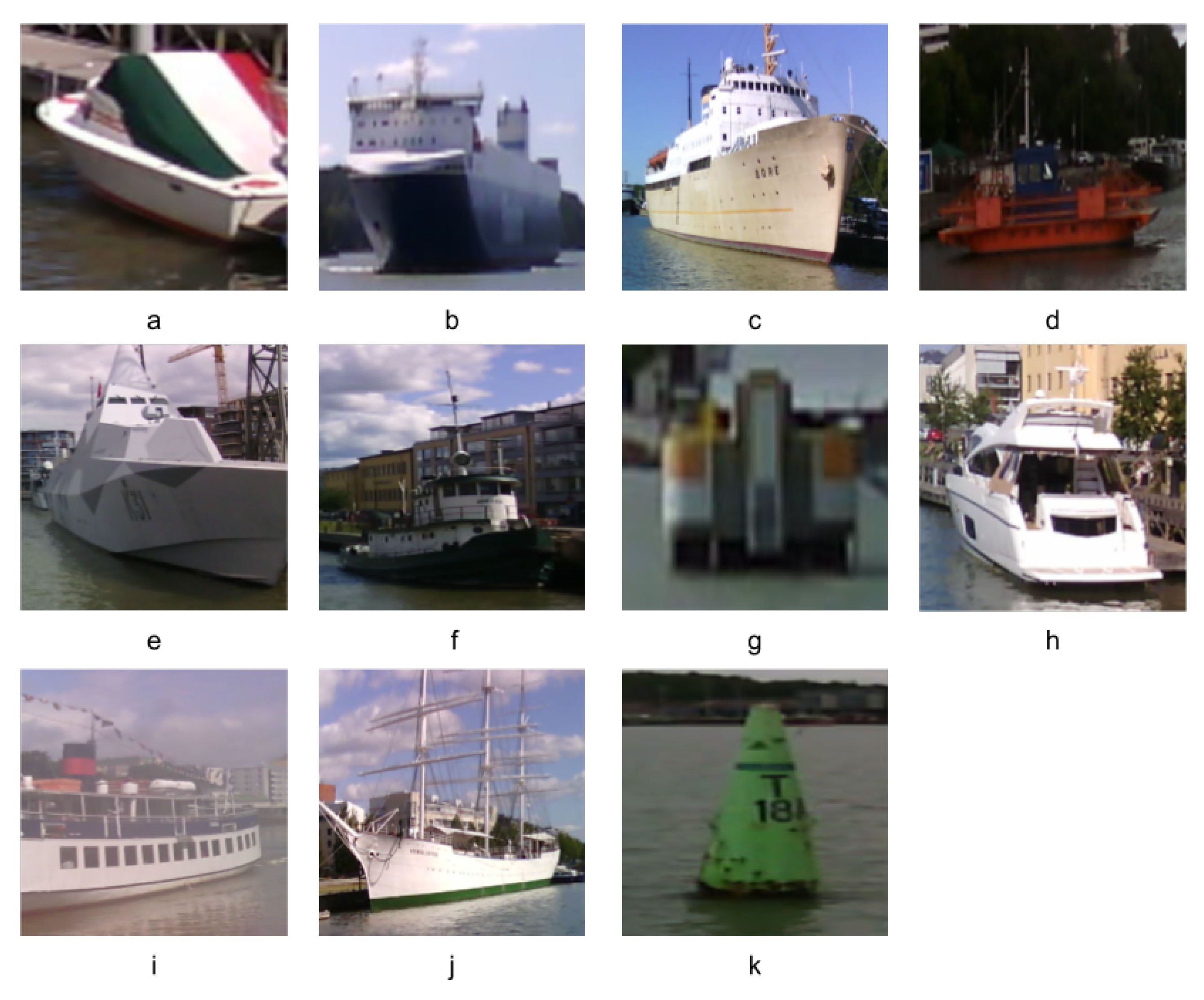
To perform the annotation task, we first investigated the captured videos and identified the vessel types that appeared most often. Due to the fact that the videos were captured at locations with a significant number of passenger ships, there is a certain level of bias for labelers towards those types of ships. This is different from the Seaships database, for instance, which comprises a higher variety of cargo ships. For the purposes of future use in machine vision, rather than using maritime terminology as such (depicting ship scale and purpose), we selected labels that had some clearly distinct visual characteristics. A visual representation of the labels is illustrated in
Figure 4. The label categories are discussed below, with more specific details for every category:
boat—rowing boats or oval-shaped boats (from a lateral perspective), or small-sized boats, visual distinction—rowing-like boats even if they possess engine power;
cargoship—large-scale ships used for cargo transportation, visual distinction—long ship with cargo containers or designed with container carrying capacity;
cruiseship—large ship that transports passengers and/or cars on longer distances (assumed at least some hundreds of km);
ferry—medium-sized ship, used to transport people and cars, a.k.a. waterbus/watertaxi, another appropriate term would be cableferry, visual distinction—it includes entrances on two opposite sides and a cabin in the middle;
militaryship—an official ship that is either military or Coast Guard and includes a special hull with antennas. For Coast Guard fleets, usually the hulls of their ships read “Coast Guard” and the military ones are dark gray/metallic/black/brown in colour;
miscboat—miscellaneous maritime vessel, visual distinction—generic boat that does not include any visual distinction mentioned in the other ship categories;
miscellaneous—identified floaters (birds, other objects floating in the water) or unidentified/unidentifiable floaters;
motorboat—primarily a speedboat, visual distinction—sleek, aerodynamic features;
passengership—medium-sized ship, used to transport people on short distances, ex. restaurant boat, visual distinction-usually it has multiple noticeable lateral windows;
sailboat—sails-propelled boat or a boat which exhibits sails, visual distinction—sails;
seamark—green/red/blue/black/yellow cone-shaped metal/plastic floater or pipe emerging from the sea.
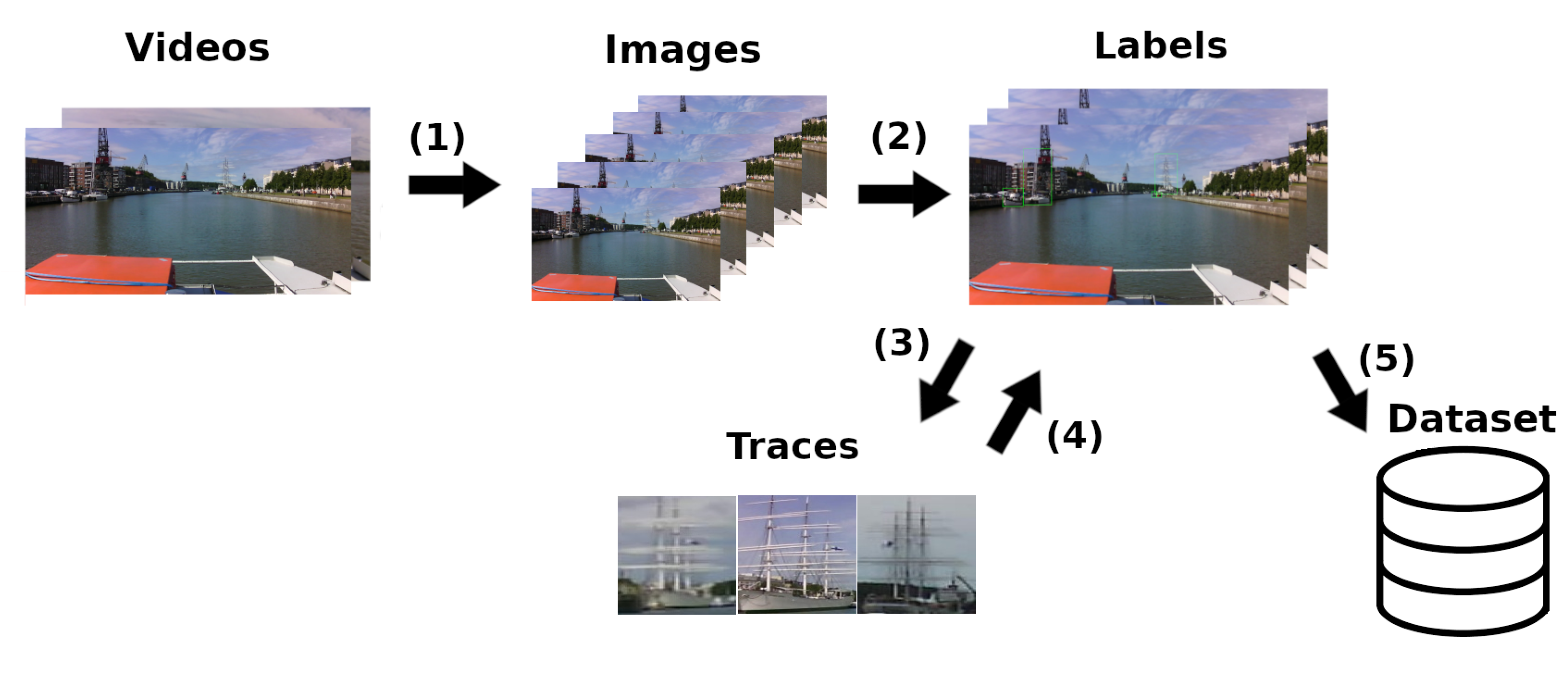
3.5. Relabelling Algorithm
The labelling was performed by multiple annotators with different backgrounds, hence some label types were interpreted differently among them. To increase the consistency of labelling, we used the continuous nature of the raw data by tracking the labels between frames using the CSRT tracker [
20]. For every labelled frame, a tracker instance was created. The aim was to track an object until the next labelled frame. At that point, the existing traces would be mapped onto the labels of the new frame, based on the
metric. During this mapping, it was assumed that labellers would not confuse seamarks with vessels, hence ship labels were not mapped onto seamarks or vice versa. More importantly, previous labels were not taken into consideration, so even if annotators gave the same object conflicting labels in different frames, these labels would still belong to the same trace as long as the tracker could identify them. For cases where the mapping could not be found, the trace would assign a new label, <
Unlabeled>, to denote that even though nothing was labeled in that specific case, the tracker indicated that the object should belong to the trace.
After a certain number of frames, either the tracker would lose the object (the most common reasons for this being object occlusion, or due to the object being either too far or exiting the frame altogether) or the tracker would have none of the defined labels mapped to it enough times (which would mean it most likely drifted onto another object). In both of those cases, the tracker was stopped and the resulting trace was saved to a file for further processing as described below.
To reduce the number of errors caused by occlusion and the tracker drifting towards other objects than the current object of interest, we performed a second tracking in the backwards direction. By comparing labels identified in the traces acquired from tracking videos in both directions, one could detect situations where traces could not be mapped onto each other. Those cases signify that the tracker was either occluded or drifted to another object, so traces required to be split into smaller sequences still, until no more conflicts could be detected.
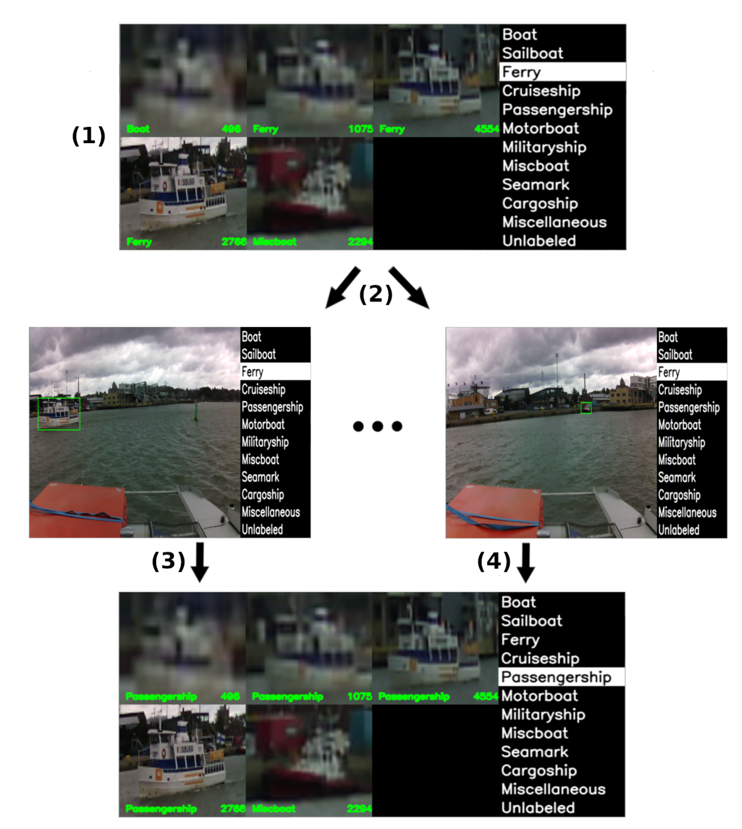
The resulting traces (after the backwards tracking) were provided as batches for relabelling. Traces containing a single entry were batched together with other singular traces from the same category. This setup was done with the purpose of preventing and removing accidental labels (mislabeling), while, at the same time, providing more information about the objects being annotated. This allowed us to accurately label even the objects at a longer distance as a consequence of tracking history. Traces obtained in this manner were then provided for relabelling as a collection of labels belonging to the same trace and annotators were asked to refine the labels so that labelling would be consistent with the labelling specifications. Singular entries that did not belong to any trace were subsequently batched together with other objects of the same category. The process described above is illustrated in
Figure 5, while the relabelling software application is depicted in
Figure 6.
3.6. Dataset Statistics
Table 4 shows the number of images of each category in our dataset and the number of annotations. The column Images represents the number of images that contain that particular object class and then the percentage of images that comprise that class follows. Then the column Objects represents the number of annotations for that particular class in the dataset, along with the percentage of objects annotated for that specific class out of all the annotated objects in the dataset. One can notice from
Table 4 that the highest representation of labels in the images from ABOships dataset is reached by three categories: motorboats (present in
of the images), sailboats (present in
of the images), and seamarks (present in
of the images). Conversely, the lowest representation is registered for cargoships (in
of the images) and miscellaneous floaters (in
of the images).
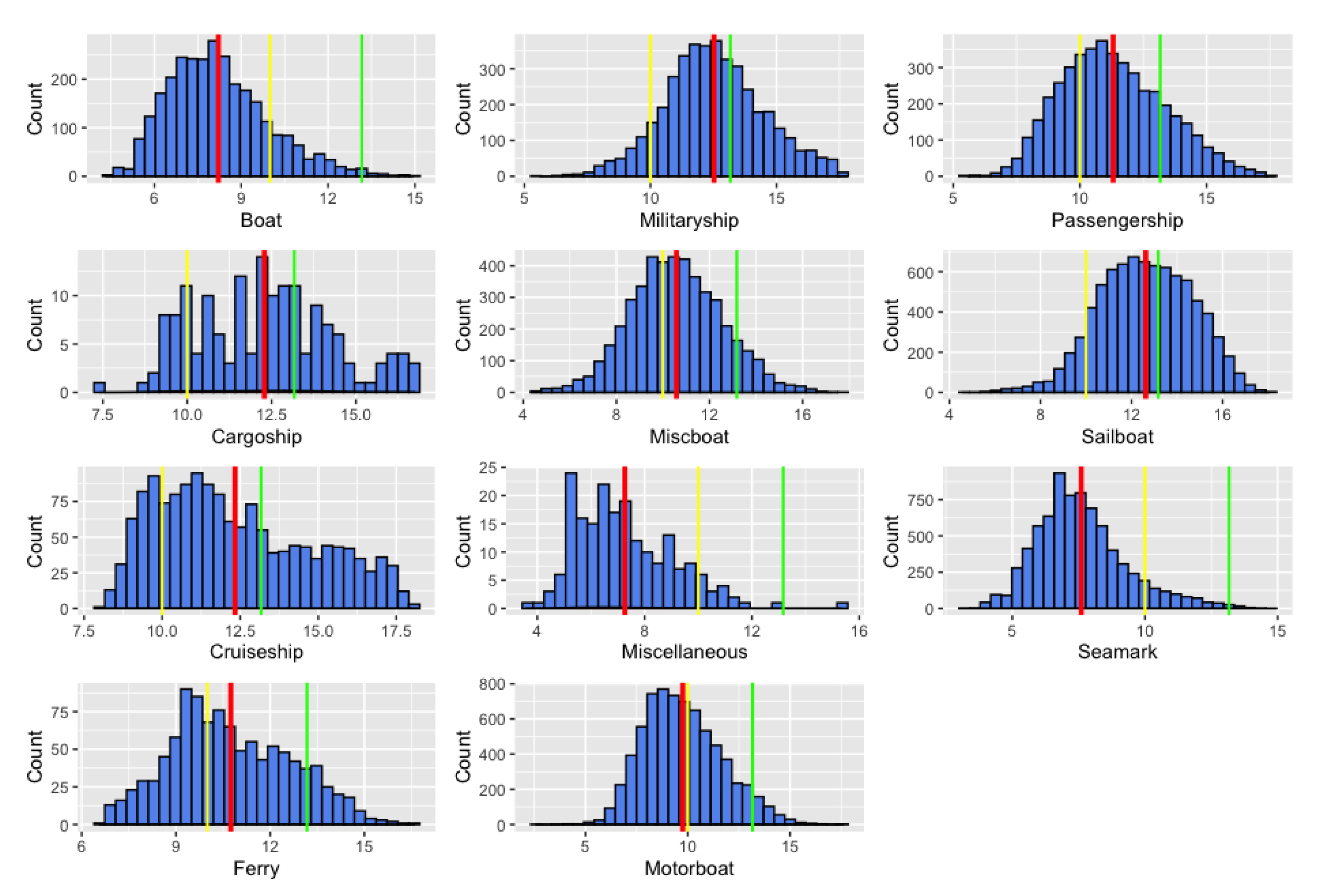
Moreover,
Figure 7 illustrates the distribution of annotated objects in our dataset based on occupied pixel area at log
-scale, for every object category, and separates every object category by size in small, medium and large objects based on the Microsoft COCO variants (small: log
(area) < 10, medium: 10 < log
(area) <
and large: log
(area) >
).
4. Results
4.1. Evaluation Criteria
To evaluate the performance of different object detection algorithms on specific datasets, one can employ various quantitative indicators. One of the most popular measures in object detection is the
IoU (Intersection of Union ), which defines the extent of overlap of two bounding boxes as the intersection between the area of the predicted bounding box
and the area of the ground truth bounding box
, over their union [
21]:
Given an overlap threshold
t, one can estimate whether a predicted bounding box belongs to the background (
) or to the given classification system (
). With this measure, one can proceed to assess the average precision (
) by calculating the precision and recall. The precision reflects the capability of a given detector to identify relevant objects and it is calculated as the proportion of detected bounding-boxes, correctly identified, over the total number of detected boxes. The recall reflects the capability of a detector to identify relevant cases and it is calculated as the proportion of correct positive predictions to all ground truth bounding boxes. Based on these two metrics one can draw a precision-recall curve, which encloses an area representing the average precision. However, in a majority of cases, this curve is highly irregular (zigzag pattern) making it challenging to estimate the area under it, i.e., the
. To address this, one can approach it as an interpolation problem, either as an 11-point interpolation or an all-point interpolation [
21].
The 11-point interpolation averages the maximum values of precision over 11 recall levels that are uniformly distributed [
21], as depicted below:
with
is calculated using the maximum precision , with a recall greater than R.
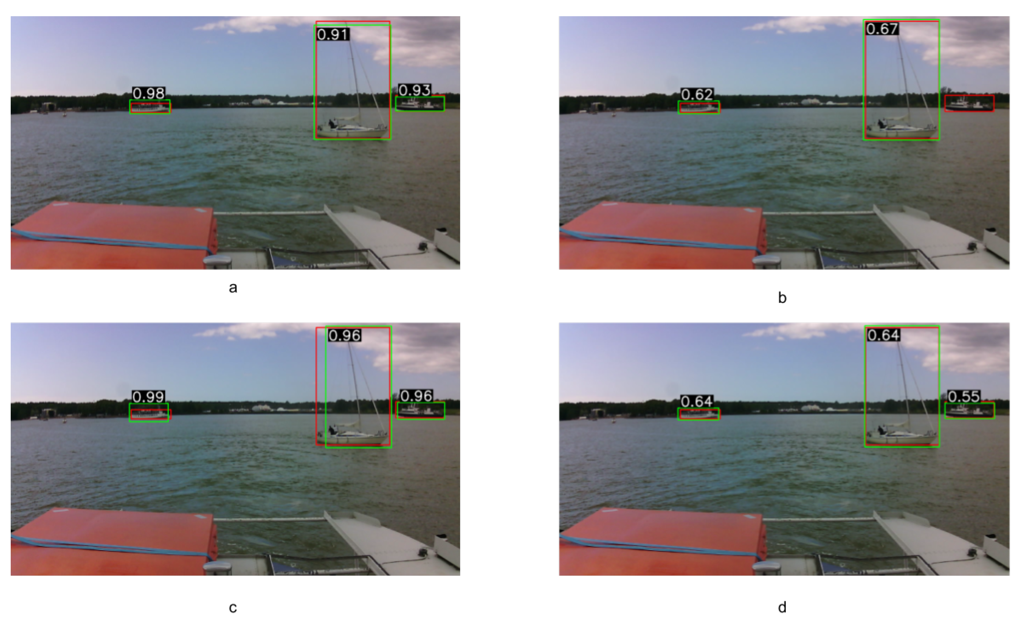
4.2. Baseline Detection
To explore the performance of CNN-based object detectors on our dataset, we focused on prevalent detectors: one-stage (SSD [
18] and EfficientDet [
22]) and two-stage detectors (Faster R-CNN [
17] and R-FCN [
23]). The detectors were previously trained on the Microsoft COCO object detection dataset, which comprises a number of 91 object categories. The training dataset contains a number of 3146 images of marine vessels. We investigated the performance of different feature extractors in the aforementioned detectors. We collect maritime vessel detection results based on SSD over different feature extractors (ResNet101, MobileNet v1, MobileNet v2). Moreover, we evaluate the performance of a new state-of-the-art detector, EfficientDet, on our dataset, which used EfficientNet D1 as feature extractor. We also evaluated two-stage detectors: Faster R-CNN and RFCN with different feature extractors. Combining all proposed detectors with the feature extractors, a total of 8 algorithms were investigated. All information regarding the specific configuration of these detectors can be found in [
24].
We estimated the performance of these algorithms in detecting maritime vessels, so we excluded seamark and miscellaneous labels from our experiments and focused on detecting vessels. Moreover, we chose images with an occupied pixel area larger than
pixels. Based on these experiments, we attained
Table 5.
Our experiments indicated that the object size impacts the detection accuracy. To corroborate this observation, we divided all vessel labels (with an occupied pixel area larger than pixels) in our datasets into three categories, based on Microsoft COCO challenge’s variants: small ( < area < ), medium ( < area < ) and large (area > ). Out of the annotated vessels with an occupied pixel area larger than pixels in our dataset, of the annotated vessels are small, are medium and are large.
Analyzing the results from our experiments, we observe that detection accuracy decreases with object size. The for best-performing detector on the ABOships dataset (Faster R-CNN with Inception ResNet v2 as feature extractor) with a registered of more than doubles in size from small () to large objects (). The second best detector on the whole dataset (EfficientDet with EfficientNet as feature extractor) however had the best performance on the large-objects category, with an . In general, detecting small objects turns out to be more difficult than larger objects given that there is less information associated with a smaller occupied pixel area. For medium-sized objects, the best performance is attained by SSD with ResNet101 as feature extractor (). For small objects, the best-performing detector, Faster R-CNN with Inception ResNet v2, outperforms the other detectors with a registered . Among the SSD configurations, best performing, in general, was the one having ResNet101 as feature extractor.
6. Discussion
Maritime vessel detection of inshore and offshore images is a topical issue in many areas, such as maritime surveillance and safety, marine and coastal area management, etc. Many of these fields require intricate management of disparate activities, which in practice often necessitate real-time monitoring. This implies, among other aspects, real-time detection of inshore and offshore ships. However, in their majority, ship detection studies and methodology are mostly concerned with either satellite or radar imagery, which can prove to be unreliable in a real-time setting. For this very reason, algorithms, and specifically CNNs, employed on waterborne imagery are especially beneficial either on their own, or in fusion architectures.
Traditional ship detection methods using either background separation or histograms of oriented gradients provide satisfactory results under favorable sea conditions. However, the complexity of the marine environment, including challenging environmental factors (glare, fog, clouds, high waves, rain etc.), renders the extraction of low-level features unreliable. Recent studies involving CNNs address this issue, but deep learning requires domain-specific datasets to produce satisfactory performance. However, public datasets specifically designed for maritime vessel detection are scarce to this day [
1]. We discuss this in more detail in
Section 2.
Performing exploratory analysis on our dataset, in comparison with other recent maritime object detection datasets (Singapore Maritime Dataset [
15], SeaShips [
3], MCShips [
19]), there are a few aspects that emerge that we discuss as follows. Comparing our dataset to the Singapore Maritime Dataset, one can notice (from
Table 3) that ABOships registers a higher number of ship types (9 vs. 6). However, considering the number of annotations per image, the Singapore dataset registers almost 3 times more annotations on average per image (
vs.
). The SeaShips dataset consists of 31,455 images, more than 3 times the image total of our dataset, but ABOships provides more annotations than the former, with a greater average number of annotations per image (
vs.
). SeaShips consists mostly of images with one annotation per image. MCShips provides a number of 13 ship categories (vs. 9 ship categories in ABOships), but only offers just over
annotations, with an average of
annotations per image, see
Table 3. We note that our dataset annotations comprise also seamarks and miscellaneous floaters in addition to the 9 ship types.
We tested our relabelling software application on the Singapore Maritime Dataset, as suggested by our reviewers, and the tracker was able to consistently map object labels from one frame to another correctly (without drifting from the object of interest to other objects), which did not always occur when we performed the tracking on the ABOships dataset. There are a few aspects that can influence the tracker’s performance and those most probably affected its performance on the ABOships dataset. First, the videos included in the Singapore Maritime dataset have a higher frame rate (30 FPS), double than those in our dataset (15 FPS). Moreover, the videos from the Onshore dataset (one part of the Singapore Maritime Dataset) have higher resolution. Videos in the Onshore dataset do not have a high density of annotations per video. Furthermore, the environment present in the images of our dataset is far more complex, including urban landscapes and complicated background, especially in the port area.
7. Conclusions
This paper provides a solution for addressing the annotation inconsistencies appeared as a consequence of manual labeling of images, using the CSRT tracker [
20]. We build traces of the images in the videos they originated from and use the CSRT tracker to traverse these videos in both directions and identify the possible inconsistencies. After this step, we employed a second round of labeling and obtained a set of
carefully annotated objects, of which 9 types of maritime vessels (boat, miscboat, cargoship, passengership, militaryship, motorboat, ferry, cruiseship, sailboat), miscellaneous floaters and seamarks.
We ensured the dataset consists of images taking into account the following factors: background variation, atmospheric conditions, illumination, visible proportion, occlusion and scale variation. We performed a comparison of the out-of-the-box performances of four state-of-the-art CNN-based detectors (Faster R-CNN [
17], R-FCN [
23], SSD [
18] and EfficientDet [
22]). These detectors were previously trained on the Microsoft COCO dataset. We assess the performance of these detectors based on feature extractor and object size. Our experiments show that Faster R-CNN with Inception-Resnet v2 outperforms the other algorithms for objects with an occupied pixel area
pixels, except in the large object category where EfficientDet registers the best performance with an
.
For future research, we plan to investigate different types of errors in the manual labelling, for cases where the labels still have inconsistencies, such as: fine-grained recognition (which renders it more difficult for human even to detect objects even when they are in plain view [
25], class unawareness (some annotators become unaware of certain classes as ground truth options) and insufficient training data (not enough training data for the annotators).
Moreover, we plan to investigate in more detail the detection of small and very small objects, including those with an occupied pixel area pixels. Furthermore, distinguishing between different vessel types in our datasets will be an essential focus as the next steps in our experiments. In order to do this, we plan to exploit transfer learning both in the form of heterogeneous transfer learning, but also homogeneous domain adaptation.
To further our research, we will employ maritime vessel tracking detectors on the original videos captured in the Finnish Archipelago and examine the impact on autonomous navigation and navigational safety.


