Learning from Nighttime Observations of Gas Flaring in North Dakota for Better Decision and Policy Making

Abstract

In today’s oil industry, companies frequently flare the produced natural gas from oil wells. The flaring activities are extensive in some regions including North Dakota. Besides company-reported data, which are compiled by the North Dakota Industrial Commission, flaring statistics such as count and volume can be estimated via Visible Infrared Imaging Radiometer Suite nighttime observations. Following data gathering and preprocessing, Bayesian machine learning implemented with Markov chain Monte Carlo methods is performed to tackle two tasks: flaring time series analysis and distribution approximation. They help further understanding of the flaring profiles and reporting qualities, which are important for decision/policy making. First, although fraught with measurement and estimation errors, the time series provide insights into flaring approaches and characteristics. Gaussian processes are successful in inferring the latent flaring trends. Second, distribution approximation is achieved by unsupervised learning. The negative binomial and Gaussian mixture models are utilized to describe the distributions of field flare count and volume, respectively. Finally, a nearest-neighbor-based approach for company level flared volume allocation is developed. Potential discrepancies are spotted between the company reported and the remotely sensed flaring profiles.

1. Introduction

In recent years, flaring the produced natural gas from the oil wells has become a commonplace practice for many operators. The United States is one of the top flaring countries in the world thanks to the rise in shale reservoir development [1,2]. North Dakota (Figure 1) is one of the top flaring states in terms of flared volume, as indicated by data from the U.S. Energy Information Administration (EIA) [3]. The consequences of flaring consist of energy waste and greenhouse gas emissions. It is desirable to obtain quantitative flaring information and track varying trends from an environmental and energy efficiency’s perspective. Since the statistics are mainly estimated and reported by the different companies, inaccuracy and imprecision are inevitably introduced.

Satellite remote sensing provides another possibility for reaching the goal of quantifying such information. For instance, the Visible Infrared Imaging Radiometer Suite (VIIRS) can help detect flares during the nighttime. In this work, the processing algorithm VIIRS Nightfire (VNF) [5] is leveraged for estimating flared gas volume. It specializes in detecting and characterizing sub-pixel hot sources and can differentiate between biomass burning and natural gas flaring [6]. The VIIRS data processing workflow is capable of picking up flares whose areas are around 1 m² (Figure 2). The main workflow is listed as follows:

• Detection of hot pixels
• Noise filtering
• Planck curve fitting
• Calculation of source area
• Calculation of radiant heat

With radiant heat evaluated, a calibration was developed for estimating flared gas volume [7], utilizing nation-level flaring data reported by Cedigaz [8]. In this paper, the developed calibration is applied to each detected flaring site in North America for estimation of flared gas volume, flare temperature, etc. In other words, the VIIRS volumes estimated for this work are largely based on the information carried by the Cedigaz reported figures.

Figure 2. The nighttime combustion source detection limits of VIIRS processing workflow [9]. The natural gas flare’s temperature is generally greater than 1500 $\mathrm{K}$.

Figure 2. The nighttime combustion source detection limits of VIIRS processing workflow [9]. The natural gas flare’s temperature is generally greater than 1500 $\mathrm{K}$.

In this work, the flaring activities in the state of North Dakota are studied with machine learning methods. Both the remote sensing interpretations and the state reporting constitute the dataset. Specifically, the VIIRS estimated volumes and data from the North Dakota Industrial Commission (NDIC) [10] are used. The NDIC is responsible for compiling the company reporting and provides the final reporting on a monthly basis. It introduced a gas flaring regulatory policy (Order 24665) in 2014 [11], with the goal of reducing flaring in three aspects: flared volume of gas, number of wells flaring, and duration of flaring from wells. The main aim of this work is therefore trying to answer the two questions below:

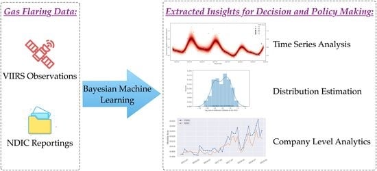
• What insights can be drawn from the VIIRS observations that could lead to better decision and policy making for the state government? Both the time series of a given entity and the whole population of entities at a given time should be studied.
• How good is the quality of the NDIC reporting (i.e., estimated and reported by different companies), by using VIIRS as a benchmark? Although uncertainties are present in the VIIRS estimates (due to the original quality of Cedigaz data as well as the temporal sampling limitations of VIIRS [7]), they are treated as the baseline.

Machine learning methods are appropriate candidates for addressing the inferential questions above, since useful structures needs to be distilled from the imperfect dataset. Throughout this paper, the effectiveness of a full Bayesian approach has been observed in learning models from gas flaring remote sensing data. The interpretability of the Bayesian approach makes it more advantageous in a high-stakes decision-making scenario (such as whether to revise gas flaring regulations) than some black box machine learning methods [12]. This choice, being a highlight of this paper, is not common in previous endeavors and deserves wider usage, especially when both the remote sensing observations and company reporting need to be studied or reconciled. Another contribution of this study is that the development of a suite of models, with both parametric and nonparametric techniques, provides guidance on how to extract insights from various angles.

2. Materials and Methods

Three types of data: VIIRS estimations (flare volumes and counts), NDIC monthly production reports, and shapefiles for North Dakota are collected for this research. The VIIRS flare inventory is compiled by the authors following the workflow outlined earlier while leveraging the calibration developed by Elvidge et al. [7]. This inventory includes monthly flare detection records in North America from March 2012 to December 2018 (both included) with the corresponding:

• Timestamps showing the specific month
• Latitudes and longitudes in WGS 84 coordinates
• Flared volume estimations in billion cubic meters ($\mathrm{bcm}$)

The monthly production reports from May 2015 to December 2018 (both included) which contain flaring information are downloaded from the NDIC [10]. There is one spreadsheet per month (starting from May 2015); each row corresponds to a well which was active in that month, and columns are for various types of information such as flared gas volume (estimated and reported by company), latitude/longitude, and field name.

The shapefiles for the counties and fields in North Dakota are downloaded from the NDIC GIS Map Server [13]. All the shapes are polygons described in NAD 27 coordinates. The shapefiles are for reverse geocoding the VIIRS detection locations to readable addresses, i.e., whether a flare is in North Dakota and which field it is located in. Thereafter, the flaring statistics from VIIRS and NDIC can be compared and contrasted at the state and field levels for a given time window.

With the help of GeoPandas [14], the procedures for extracting county and field names are listed as follows:

• Store the VIIRS observations as a geospatial data object, with their original coordinates in WGS 84.
• Store the shapefile as a geospatial data object, with its original coordinates in NAD 27.
• Transform all the geometry coordinates in the shapefile to WGS 84.
• Perform a spatial join of the two data objects to obtain the field information for each flare, if a field and the flare share any boundary or interior point.

The VIIRS records that are within the state of North Dakota are located (Figure 3a) and chosen for the study. Both the NDIC well map and VIIRS flare map showing the study area are graphed and presented in Figure 3b.

In this work, Bayesian machine learning is utilized to develop the data-driven models for the purpose of insights extraction and decision/policy making. In a nutshell, it utilizes probability theory to set up a formal procedure for learning from data [15]. In a certain learning task, Bayesian models provide full joint probability distributions $p(\mathcal{D},\mathbf{\theta })$ over observable data $\mathcal{D}$ and unobservable model parameters $\mathbf{\theta }$. The goal is to find the posterior distribution $p(\mathbf{\theta }\mid \mathcal{D})$, i.e., a probability distribution of the parameters conditioned on the historical observations. Once the posterior is obtained, depending on the parameter and model’s interpretability, the developed model with a set of highly probable parameter values can be deployed to make inferences or predictions. The posterior is derived through Bayes’ theorem:

$$\begin{array}{}\mathrm{(1a)}& p(\mathbf{\theta }\mid \mathcal{D})& ={\displaystyle \frac{p(\mathcal{D}\mid \mathbf{\theta })p\left(\mathbf{\theta }\right)}{p\left(\mathcal{D}\right)}}\mathrm{(1b)}& & ={\displaystyle \frac{p(\mathcal{D}\mid \mathbf{\theta })p\left(\mathbf{\theta }\right)}{\int p(\mathcal{D}\mid {\mathbf{\theta }}^{\prime })p\left({\mathbf{\theta }}^{\prime }\right)\mathrm{d}{\mathbf{\theta }}^{\prime }}}\end{array}$$

where $p(\mathcal{D}\mid \mathbf{\theta })$ is the likelihood or observation model which denotes how likely the data are when conditioned on a certain set of parameters, and $p\left(\mathbf{\theta }\right)$ is the prior which models the probability of the parameters before observing any data. Thus, the prior is used to encode domain expertise.

Many of the integration problems central to Bayesian analysis, including the denominator in Equation (1b), are analytically intractable. A category of sampling algorithms, known as Markov chain Monte Carlo (MCMC), can be applied to approximate these quantities [16], helping achieve the goal of computing the posterior distributions. The idea is to construct Markov chains with specific target distributions, and allowing the chains to traverse the sample space while collecting random samples. The integral can then be approximated using the Monte Carlo principle.

Hamiltonian Monte Carlo (HMC), originally proposed in [17], currently outperforms the other algorithms in the MCMC category and is chosen as the main sampling strategy in this paper. Specifically, the No-U-Turn Sampler (NUTS) introduced in [18], which is an extension to HMC, is employed for sampling from posterior distributions. In the following sections, all the machine learning studies are performed under the same Bayesian framework; however, the probabilistic building blocks (i.e., prior and likelihood) are bespoke. The majority of this work is implemented by leveraging PyMC3 [19], which encapsulates the NUTS sampler.

3. Results

In this section, three scenarios are studied and the results are presented correspondingly:

• Time series analysis, where the temporal structure is harnessed for exploring the patterns and trends in flaring performance;
• Cross-sectional data analytics, where the VIIRS observations collected for one point or a period of time (such as a certain month or quarter) are summarized for distributional insights;
• Company level monitoring and analysis, where flare ownership connecting detections with companies is established. The NDIC and VIIRS reporting for a given company can then be compared and contrasted.

3.1. Flaring Time Series Analysis

For the task of inferring flaring strategies and behaviors, the flaring data should be inspected from the time series’ perspective. To recognize the patterns and trends from the time series where measurement and estimation errors are present, Gaussian process (GP) makes principled handling of uncertainty and interpretation possible [20,21] and is employed in this section. A GP can be viewed as a distribution over functions. It is well established as a Bayesian machine learning method, and many data analytics methods such as kriging and Kalman filters correspond to specific forms of GP [22].

GPs can help organizations such as the NDIC to determine whether a given entity meets the flaring reduction targets or not, in a entirely probabilistic framework (e.g., under a predefined confidence level). For the learning tasks in this paper, inferences of the underlying latent processes are conducted directly in the function space. GP is utilized as a prior for the unknown functions. A GP is completely specified by its mean function $m\left(\mathbf{x}\right)$ and kernel $k(\mathbf{x},{\mathbf{x}}^{\prime })$, and the latent function $f\left(\mathbf{x}\right)$ distributed according to a GP is denoted by:

$$f\left(\mathbf{x}\right)\sim \mathcal{G}\mathcal{P}\left(m\left(\mathbf{x}\right),k(\mathbf{x},{\mathbf{x}}^{\prime })\right),$$

(2)

where $\mathbf{x}$ and ${\mathbf{x}}^{\prime }$ are the inputs, and the input space $\mathcal{X}\subseteq {\mathbb{R}}^1$ is the time domain. $\mathcal{G}\mathcal{P}$ denotes the Gaussian process. In this work, the mean functions are always set to be zero. The kernels adopted include the Matérn kernel with $\nu =5/2$, the standard periodic kernel, and the white noise kernel.

3.1.1. Modeling VIIRS Detection Count

The number of satellite-detected flares reflects flaring magnitude in terms of emerging combustion sources. Since the satellite could miss some flaring events due to resolution and measurement errors, the inference task is to investigate how the “true” count varies over a given time period. By exploiting GP, the model is specified through Expressions (3a)–(3f) (numbered as Model 3). Essentially, the latent process is modeled using a Poisson process whose intensity is assigned a GP prior:

$$\begin{array}{}\mathrm{(3a)}& \ell \sim \mathrm{Gamma}(2,1)\mathrm{(3b)}& \eta \sim \mathrm{Half}-\mathrm{Cauchy}\left(5\right)\mathrm{(3c)}& k={\eta }^2\times k_{\mathrm{MATÉRN}52}(x,x^{\prime };\ell )\mathrm{(3d)}& f\sim \mathcal{GP}(0,k)\mathrm{(3e)}& {\lambda }_i=\exp \left(f\left(x_i\right)\right)\mathrm{(3f)}& C_i\sim \mathrm{Poisson}\left({\lambda }_i\right)\end{array}$$

where:

ℓ  

is the lengthscale for the Matérn kernel;

$\eta$  

is the marginal deviation controlling the latent functions’ magnitudes in the output space;

k   

is the kernel for the GP;

f   

is the latent process;

${\lambda }_i$ 

is the flaring intensity (unobserved “true” count) of month i. Since ${\lambda }_i$ is always positive, the natural exponential function is applied to f;

$C_i$ 

is the reported count from VIIRS in month i.

Following the reverse geocoding discussed earlier, the model is tested with the data from the Blue Buttes Field (Figure 4), which is a major producing field [23]. The VIIRS observations are used which trace back to 2012. The posterior distributions (defined in Equation (1a) for ℓ and $\eta$) and trace plots (showing the sampling progress for ℓ and $\eta$) are displayed in Figure 5. To test for model convergence, four Markov chains are set up to run in parallel. Their sampling progresses are plotted with different colors, and it is clearly shown that well mixing and convergence of the four chains are achieved. This indicates that the model is confident with its learning outcomes (characteristics of the field), using the observations from the field. In other words, the inference results are valid and robust.

The posterior predictive samples for the underlying process of flare count (${\lambda }_i$) are demonstrated in Figure 6, which depicts the trend distinctly. The colored ribbons have the coverage below for the posterior samples:

• The lightest ribbon (the widest interval for a certain x) represents the 1st to 99th percentile;
• The darkest ribbon (in the center for a certain x) represents the 49th to 51st percentile.

In addition, thirty samples (inferred functions) are drawn from the GP posterior and plotted as thin lines. Neither the inferred main trend nor any of the sample functions go through all of the observed data points, indicating that the outcome is not overfitting. Because the observations are never generated in a noise-free environment, any model that fits perfectly to the data are overfitting and fragile. By employing the utility of full Bayesian inference in training a GP model, the inference results reveal the most dominant trend that is compatible with both the model assumptions and the imperfect data.

Reducing the number of flaring wells is one of the three goals of the regulatory policy introduced by the NDIC [11]. However, a flaring device is sometimes associated with more than one wellhead, leading to uncertainties in the company reported flaring well count. Since the detection count can be used as a surrogate for the well count, this model helps infer whether a given entity makes efforts to achieve the target. The state level trends can also be revealed if the corresponding data are fed into the model: the posterior distributions and trace plots are displayed in Figure 7, and the inferred varying trends are demonstrated in Figure 8.

Through the posterior predictive ribbons, important patterns are uncovered; for example, one peak exists around summertime every year. This could be due to the lack of demand for natural gas in summer and therefore more flaring activities are spotted.

By employing a Bayesian approach, both flexibility (for automation) and interpretability (for modification) are obtained in the model building process. For the former, with the same model specification, the state government can gain insights into the difference between certain fields and the whole state, with their corresponding dataset. This makes it possible to automate the analysis for every entity in each level. In the case of interpretability, as an example, the constructed model incorporating a Poisson likelihood can serve as the first modeling attempt because the Poisson distribution has only one parameter. If the state government would like to consider the effects of overdispersion, Expression (3f) can be changed to other observation models such as the negative binomial likelihood. This interpretability of the developed model (due to its generative nature) is the reason why it is more advantageous than other approaches such as smoothing splines.

3.1.2. Modeling Scale Factor between VIIRS and NDIC

Estimated flared gas volumes are provided via both NDIC and VIIRS. Data from the two sources are visualized in Figure 9, which demonstrate a positive association. Because the satellite imagery processing is based on a consistent workflow, the scale factor $\beta$ between VIIRS and NDIC (assuming $\mathrm{NDIC}=\beta \times \mathrm{VIIRS}$) can serve as an indicator of whether the NDIC reporting is consistent, when the time series of a given entity is inspected and the latent process of $\beta$ is inferred. The model for inferring the scale factor variations is specified through Expressions (4a)–(4n) (numbered as Model 4):    

$$\begin{array}{}\mathrm{(4a)}& \hfill {\ell }_{\mathrm{MAT}}& \sim & \mathrm{Gamma}(8,2)\hfill \mathrm{(4b)}& \hfill {\eta }_{\mathrm{MAT}}& \sim & \mathrm{Half}-\mathrm{Cauchy}\left(5\right)\hfill \mathrm{(4c)}& \hfill T& \sim & \mathcal{N}(12,1)\hfill \mathrm{(4d)}& \hfill {\ell }_{\mathrm{PER}}& \sim & \mathrm{Gamma}(4,3)\hfill \mathrm{(4e)}& \hfill {\eta }_{\mathrm{PER}}& \sim & \mathrm{Half}-\mathrm{Cauchy}\left(5\right)\hfill \mathrm{(4f)}& \hfill \nu & \sim & \mathrm{Gamma}(2,0.1)\hfill \mathrm{(4g)}& \hfill {\widehat{\sigma }}^2& \sim & \mathrm{Half}-\mathrm{Cauchy}\left(5\right)\hfill \mathrm{(4h)}& \hfill k_{\mathrm{MAT}}& =& {\eta }_{\mathrm{MAT}}^2\times k_{\mathrm{MATÉRN}52}(x,x^{\prime };{\ell }_{\mathrm{MAT}})\hfill \mathrm{(4i)}& \hfill k_{\mathrm{PER}}& =& {\eta }_{\mathrm{PER}}^2\times k_{\mathrm{PERIODIC}}(x,x^{\prime };T,{\ell }_{\mathrm{PER}})\hfill \mathrm{(4j)}& \hfill k_{\mathrm{WN}}& =& k_{\mathrm{WHITENOISE}}(x,x^{\prime };\delta =1e-6)\hfill \mathrm{(4k)}& \hfill f& \sim & \mathcal{GP}(0,k_{\mathrm{MAT}}+k_{\mathrm{PER}}+k_{\mathrm{WN}})\hfill \mathrm{(4l)}& \hfill {\beta }_i& =& \exp \left(f\left(x_i\right)\right)\hfill \mathrm{(4m)}& \hfill {\mu }_i& =& {\beta }_i\times {\mathrm{VIIRS}}_i\hfill \mathrm{(4n)}& \hfill {\mathrm{NDIC}}_i& \sim & \mathrm{Student}-t(\nu ,{\mu }_i,1/{\widehat{\sigma }}^2)\hfill \end{array}$$

where:

${\ell }_{\mathrm{MAT}}$    

is the lengthscale for the Matérn kernel;

${\eta }_{\mathrm{MAT}}$    

is the marginal deviation for the Matérn kernel;

T     

is the period for the periodic kernel;

${\ell }_{\mathrm{PER}}$   

is the lengthscale for the periodic kernel;

${\eta }_{\mathrm{PER}}$   

is the marginal deviation for the periodic kernel;

$\nu$     

is the degrees of freedom for the Student-t likelihood;

${\widehat{\sigma }}^2$   

controls the inverse scaling parameter for the Student-t likelihood;

$k_{\mathrm{MAT}}$     

is the Matérn kernel;

$k_{\mathrm{PER}}$     

is the periodic kernel;

$k_{\mathrm{WN}}$     

is the white noise kernel;

f     

denotes the latent process, which is distributed according to a GP whose kernel is the sum of three kernels;

${\beta }_i$    

is the underlying scale factor between VIIRS and NDIC of month i. Since this scale factor is bounded to be positive, the natural exponential function is applied to the latent process;

${\mathrm{VIIRS}}_i$ 

is the VIIRS reported volume of month i;

${\mu }_i$    

denotes the unobservable “true” flared volume of month i;

${\mathrm{NDIC}}_i$ 

is the NDIC reported volume of month i, which is modeled using a Student-t likelihood.

The justification for choosing a Student-t likelihood is to make the model specification be robust to noisy data points with potentially many outliers. Currently, companies have to estimate or measure the flared volume by their own procedures, compile the figures, and submit the reports. In this process, inaccuracies and occasional errors are inevitable. The heavy tail of Student’s t-distribution makes it an excellent candidate to manage those circumstances. Similarly, adopting the half-Cauchy priors as well as GP as a nonparametric regression technique makes the system robust and generic to as many entities and situations as possible. The reason behind including a periodic kernel is to scrutinize if any seasonal patterns exist. By maintaining a full Bayesian workflow, this choice lets the data speak for itself (whether seasonality prevails or not) instead of compelling seasonality to be present in the final inference results.

Figure 9. Visualizations of both the NDIC and VIIRS observations at the state level. The left figure presents the time series. The right figure displays the scatterplot using each month’s data points.

Figure 9. Visualizations of both the NDIC and VIIRS observations at the state level. The left figure presents the time series. The right figure displays the scatterplot using each month’s data points.

With the state level reporting, the macroscopic consistency of the NDIC data is examined by using the VIIRS as a benchmark. The posterior distributions and trace plots are displayed in Figure 10. The inferred latent process of the scale factor variations is visualized through the posterior samples (Figure 11). In general, the NDIC reported volumes are less than the VIIRS reported quantities. It is only when the overall flaring intensity was small (manifested by the smaller point size) that the NDIC reported volumes are larger than VIIRS. More interestingly, it becomes apparent that the scale factor ${\beta }_i$ always declines within every year. The inferred process from the second quarter to the third quarter can be envisioned as a “seesaw,” where July is the middle pivot point and the months after July always observe a falloff. Within a given year, the NDIC reported volumes might still increase; however, the scale factor decreasing suggests that much greater flaring magnitude was captured by the satellite sensors.

Since the state level statistics were compiled based on the company reports, it is interesting to study whether the seasonal behavior is universal across all the entities. Indeed, if data from the Blue Buttes Field are used to fit the same model, quite consistent scale factors are inferred. The posterior distributions and trace plots are displayed in Figure 12. The trend of scale factor variations (${\beta }_i$) is visualized in Figure 13, where no apparent seasonal patterns are picked out by the inference process. The large uncertainties around early 2016 are possibly caused by the truncation effects instead of reporting quality issues. That is, when the flares become intermittent and infrequent (could be due to sudden increase of gas consumption on site, rising gas prices, anti-flaring regulations, etc.), they are easily missed by the satellites. Based on the discussions above, the state government should have a good reason to believe that some entities might have underreported their flared volumes, especially after midyear. By fitting the model to other major producing fields’ observations, the ones which exhibit the seesaw behaviors can be determined.

3.1.3. Predicting NDIC Reported Volume

Once the model hyperparameters are learned, GP is fully capable of making predictions. This section tackles the problem of predicting the NDIC reported volume based on the forecasted scale factor to be applied on VIIRS. After the workflow for rapid satellite detection/estimation becomes available (i.e., new interpretations become available on a monthly basis), this model makes it possible for the flared volume being estimated before company reports are received and compiled (which usually takes two months).

The predictions of the scale factor variations are demonstrated in Figure 14. The widening percentile ribbons show that the seasonal patterns might take place again and the uncertainties are large. If point predictions as opposed to prediction intervals are required, the posterior mean, mode, or median can be employed to construct the “best” function. The intervals, however, showcase the difficulties in predicting the future and the necessity of quantifying the uncertainties.

3.2. Distribution Approximation

Besides time series modeling, flaring data can also be studied in a cross-sectional setting. More specifically, this section addresses the problem of summarizing the flaring associated quantities’ distribution among all the fields, for a given point of time (e.g., month or quarter). The dataset is unlabeled in this case:

$$U=\left\{x_1,x_2,\dots ,x_N\right\},$$

(5)

where $x_i$, $i=1,2,\cdots ,N$, is the observation for the i-th field. The learning target is a conditional probability distribution $P_{\mathbf{\theta }}(x\mid z)$, where $\mathbf{\theta }$ are the unknown parameters and z is some latent structure.

The practical scenarios for such cross-sectional studies include profile comparison with previous times and summarizing the population whilst looking for hidden groups. The inference results, in a form of distributional insights, will be informative for the state government to gain further understanding of the status quo and develop policies.

3.2.1. Modeling VIIRS Detection Count

In Section 3.1.1, the time series of VIIRS detection count for a given field is the subject of modeling. This section addresses the problem of approximating the distribution of a given month’s count data for all of the fields. Because non-negative integer values are analyzed, the four likelihoods below are compared for several randomly selected months’ records:

• Poisson
• Negative binomial
• Zero-inflated Poisson (ZIP)
• Zero-inflated negative binomial (ZINB)

Zero-inflated models are experimented with because many fields in North Dakota did not show up on VIIRS in a given month. Through posterior predictive checks, it is found that the negative binomial model provides the best approximation to the data generating process, and thus is employed in this work. It is specified through Expressions (6a)–(6c) (numbered as Model 6):

$$\begin{array}{}\mathrm{(6a)}& \hfill \mu & \sim & \mathrm{Gamma}(2,1)\hfill \mathrm{(6b)}& \hfill \varphi & \sim & \mathrm{Exponential}\left(1\right)\hfill \mathrm{(6c)}& \hfill C_j& \sim & \mathrm{NegBinomial}(\mu ,\varphi )\hfill \end{array}$$

where $C_j$ is the detection count for the j-th field. Because the negative binomial distribution characterizes a Poisson random variable whose mean is distributed according to a gamma distribution, the learned parameters are very interpretable:

• $\mu$ indicates the mean intensity from the perspective of flare count, analogous to the interpretation of a Poisson’s mean. The larger the value of $\mu$, the greater number of combustion sources are present on average.
• $\varphi$ is the overdispersion parameter indicating the diversity of the fields in North Dakota. Specifically, ${\mu }^2/\varphi$ is the additional variance above that of a Poisson with mean $\mu$. The smaller the value of $\varphi$, the more fields with a huge number of flares exist.

To showcase this model’s performance in learning from data, the observations from October 2018 are collected. There are 506 producing fields altogether. The histogram of the detection count for all of the fields is displayed in Figure 15.

After fitting Model 6, the posterior distributions and trace plots are displayed in Figure 16. The parameter estimates are presented in

Table 1. Parameter estimates of field detection count distribution.

Parameter	Variable	Point Estimate	90% Credible Interval
$\mu$	Intensity	1.005	(0.814, 1.200)
$\varphi$	Diversity	0.168	(0.135, 0.202)

.

The point estimate for the intensity $\mu$ is remarkably small ($\widehat{\mu }\approx 1$), which is due to the model being fed with a large number of zeros. Because the tail of the histogram reaches far beyond $\widehat{\mu }$ (Figure 15), posterior predictive checks are conducted to examine Model 6’s compatibility with the data.

Figure 17 visualizes the results of the check, i.e., the histograms for the original observations and for all of the posterior predictive simulations are plotted. Each set of the possible parameter values ($\mu$ and $\varphi$) is used to generate one synthetic dataset for the fields in North Dakota. There are 12,000 datasets in total, since each of the four Markov chains is set up for 3000 iterations. Every individual histogram is graphed using an unfilled line chart.

Since there does not exist any obvious discrepancies between the raw observations and simulation results, the model is found to be compatible with the dataset. To closely examine the tail of the distribution where the count becomes larger than zero, the y-axis is clipped for a zoomed-in view (Figure 18), in which some disagreement is noticed. A rigidity of this model is that it would still be surprised by a high detection count such as $C_j\ge 20$, even with the relatively large overdispersion effects ($\widehat{\varphi }\approx 0.2$). On the whole, the explainability, efficacy, and simplicity of Model 6 make it a recommended choice for summarizing the detection count distribution. The practical use cases are discussed in Section 4.2.

3.2.2. Modeling Flared Volume

Apart from detected flare count, estimated flared volume provides another critical facet of the flaring landscape. In this section, a distributional summary of the VIIRS estimated flared volumes for various fields is acquired. Specifically, all the 152 fields’ cumulative flared volumes from the fourth quarter of 2018 are assembled for investigation. The original absolute volumes in $\mathrm{bcm}$ are greatly skewed (Figure 19). Consequently, the order of magnitude of the flared volume is computed for each field and then used for study:

$$L_i=log\left(F_i\right),$$

(7)

where $L_i$ is the magnitude of flared volume, and $F_i$ is the VIIRS reported volume in $\mathrm{bcm}$, both of which belong to the i-th field. Base e is used for the logarithm. Figure 20 exhibits the univariate distribution of the magnitudes exploiting rug plot, histogram, and kernel density estimate (KDE).

All three visualization tactics agree that a single Gaussian would be a poor approximation to the underlying density. Therefore, a Gaussian mixture model (GMM) is utilized to represent the population. The number of components K needs to be specified and $\forall K\in \{2,\cdots ,7\}$ are assessed. Larger numbers of components are avoided for better interpretability of the modeling results. The mixture model is defined through Expressions (8a)–(8h) (numbered as Model 8):

$$\begin{array}{}\mathrm{(8a)}& \hfill \mathit{\alpha }& =& ({\alpha }_1,\dots ,{\alpha }_K)=6·{\mathbb{𝟙}}_K\hfill & \mathrm{(8b)}& \hfill \mathbf{w}& \sim & \mathrm{Dirichlet}\left(\mathit{\alpha }\right)\hfill & \mathrm{(8c)}& \hfill l_1& =& \min \{L_1,\cdots ,L_n\}\hfill & \mathrm{(8d)}& \hfill l_2& =& \max \{L_1,\cdots ,L_n\}\hfill & \mathrm{(8e)}& \hfill {\tilde{\mu }}_k& =& l_1+(k-1)\left(\frac{l_2-l_1}{K-1}\right),\hfill & k=1,\cdots ,K\mathrm{(8f)}& \hfill {\mu }_k& \sim & \mathcal{N}({\tilde{\mu }}_k,2),\hfill & k=1,\cdots ,K\mathrm{(8g)}& \hfill {\sigma }_k& \sim & \mathrm{Half}-\mathrm{Normal}\left(2\right),\hfill & k=1,\cdots ,K\mathrm{(8h)}& \hfill L_i& \sim & \sum _{j=1}^K{w}_j\mathcal{N}({\mu }_j,{\sigma }_j)\hfill & \end{array}$$

where:

$\mathit{\alpha }$    

is the vector of concentration parameters for the Dirichlet distribution;

$\mathbf{w}$    

is the vector of mixture weights (i.e., mixing proportions) which is assigned a Dirichlet prior. This prior with every value inside $\mathit{\alpha }$ being 6, is a weakly informative prior, expecting any $w_k$ inside $\mathbf{w}$ could be greater or less than the others;

$l_1\mathrm{and}{l}_2$ 

are the lower and upper bound for ${\left\{L_i\right\}}_{i=1}^n$, respectively;

${\tilde{\mu }}_k$    

is the prior for the location of the k-th mixture component, and ${\left\{{\tilde{\mu }}_k\right\}}_{k=1}^K$ represent the K evenly spaced points in $[l_1,l_2]$;

${\mu }_k$    

is the mean for the k-th Gaussian component;

${\sigma }_k$    

is the standard deviation for the k-th Gaussian component.

For each of the six different K’s, well mixing and convergence of the Markov chains are achieved. The inference results for different number of components are visualized through Figure 21, where both the inferred mean Gaussian components and fifty posterior samples are graphed.

By inspecting the similarities between the posterior mean density and the KDE, it is evident that the multimodal features are described effortlessly by using a mixture of Gaussians. Although a larger K (e.g., $K=6$ or $K=7$) yields more resemblances between the posterior density and KDE, more fluctuations and stochasticity are manifested in the posterior samples, suggesting overfitting. The widely applicable information criterion (WAIC) [24] is used to choose the best K. WAIC provides an estimate for the out-of-sample KL divergence [25], and therefore a lower value is better. The comparison results for the six models are summarized in Figure 22.

Considerable overlaps exist for all of the models when the standard error is taken into account. Considering that $K=2$ yields the most parsimonious model with the smallest WAIC, the two components GMM is chosen for this dataset following Occam’s razor. The implications of this are discussed in Section 4.3.

3.3. Company Level Monitoring and Analytics

In previous sections, the satellite-detected flaring statistics are compiled and studied at the state and field levels. For the state government to obtain more granular insights in a regulatory context, it is beneficial to achieve company level monitoring and analytics by making use of remote sensing data. Currently, only the latitudes and longitudes of company wells (points) are available through the NDIC. Due to the lack of a company leases (polygons) shapefile, a nearest-neighbor-based approach is developed and summarized as Algorithm 1. Essentially, the satellite-detected flares are assigned to the closet companies, based on the well locations and corresponding time window. In the algorithm, the function SearchClosestCompany($·$) returns the closest company (${\mathrm{OP}}_j$) for every detected flare and the calculated distance ($d_j$) between them. Haversine distance is computed and thus the Earth radius ($R_E$) is required as an input. For speedup on the search, a ball tree is leveraged in the function implementation.

Due to the high-stakes nature in the assigning process, some logics are put in place for deciding whether to keep or drop the company assignment. The design is as follows: the assignment is immediately stored or rejected, when $d_j$ is significantly small or large, respectively. The assignment for the case of $d_{\mathrm{SECURE}}\le d_j\le d_{\mathrm{CUTOFF}}$ will be kept only when the flare and company are situated on the same township, range, and section.

Algorithm 1: Nearest-Neighbor-Based Flare Owner Assignment

The effectiveness of Algorithm 1 is tested with the VIIRS and NDIC flaring data, using the inputs below:

$$\begin{array}{}\mathrm{(9a)}& \hfill d_{\mathrm{SECURE}}& =300 \mathrm{m}\hfill \mathrm{(9b)}& \hfill d_{\mathrm{CUTOFF}}& =800 \mathrm{m}\hfill \mathrm{(9c)}& \hfill R_E& =6371 \mathrm{k}\mathrm{m}\hfill \end{array}$$

Some companies, for example Company A and Company B, manifest strong associations between the VIIRS and NDIC volumes (Figure 23). A linear model (${\mathrm{NDIC}}_i=\alpha +\beta \times {\mathrm{VIIRS}}_i$) is fitted by ordinary least squares, the results of which are presented in the legend. Because the intercepts are close to zero, these companies’ reporting show consistency with the VIIRS reporting up to a scale factor. There exists diversity in the scale factors among the companies.

However, some companies, for example Company C and Company D, are found to show discrepancies between the VIIRS and NDIC volumes (Figure 24). Through close examination of the scatterplots, the poor fits of the linear model are partially caused by some data points being “pushed down” toward the x-axis. The company time series are plotted (Figure 25) and indicate that the pattern is caused by the company-reported volumes leveling off for certain periods of time. The VIIRS time series show that there were stronger variations of flaring intensity for those times. The reporting from Companies A and B, however, demonstrates better match with the remote sensing observations (Figure 26). By employing the introduced workflow, a flag can be raised when these types of datasets are present, achieving the first step in anomaly detection for company profiles. Considering the possibility of misassigning the satellite-detected flares to the companies, in order to nail down any decisions with regard to company reporting quality, great cautions must be applied, which are discussed in Section 4.4.

4. Discussion

This section discusses the implications and potential use cases of the Bayesian learning models, as well as the caveats in applying nearest neighbor analysis to the companies.

4.1. GP’s Attractive Traits

The Gaussian process models demonstrate full capability of harnessing the temporal structure from flaring time series at different levels. This provides a huge potential for extracting insights from noisy monthly data streams. In fact, the elegant properties of GP make it a natural choice to tackle a family of problems which share the challenges and requirements below:

• The observations contain much noise, for example, the estimation and measurement errors.
  In the context of flaring data, companies estimate and self-report the volumes; satellites inevitably miss some events or overestimate some flares’ duration. Nonetheless, knowledge about the underlying “true” process (i.e., the dominating trend) is desirable in many decision-making situations and helps with anomaly detection from flaring profiles.
• The observations for a given entity are time series.
  The temporal structure is intrinsic to the dataset, and observations collected at different times are not independent samples. For example, the adjacent months’ observations are typically strongly correlated, while the distant months (such as five years apart) might be weakly associated.
• A probabilistic model is required.
  When inferring the latent process, a posterior distribution of probable functions is preferable over one “best” function (for instance, the best gradient boosting regressor or the best neural network classifier under a certain type of performance measure).
• A generic framework that embraces automation is beneficial.
  With more than 200 companies and 500 producing fields in North Dakota, Bayesian nonparametric models are more advantageous than parametric techniques for automated insights extraction, e.g., computing every entity’s KPIs based on the inference results. In a parametric setting, each entity needs its own form of parametric model and the underlying implications could be contrasting, which poses challenges to the development of automation pipelines.

4.2. Use Cases of Negative Binomial Model

Model 6 is believed to be valuable in the two use cases below:

• $\mu$ and $\varphi$ for the most recent month can be estimated via training Model 6 with the latest VIIRS observations. A comparison study can be conducted by comparing the parameter estimates with those from earlier times, in light of uncertainties characterized by the corresponding credible intervals. Concerning the example in Section 3.2.1, the inference results can be compared with either August/September 2018 or October 2016/2017. From the study, it helps answer questions such as whether more fields with huge flaring magnitude are identified (indicated by a smaller $\varphi$), or if there are more detected flares on average (indicated by a larger $\mu$).
• Following the model training process, it is advisable to carry out the posterior predictive checks to identify any discrepancies between the raw observations and simulations, the results of which are exhibited in Figure 17 and Figure 18. The fields that show large deviations from the simulated observations, especially those on the far tail (e.g., $C_j\ge 20$), are worth further investigation. For instance, to inspect whether the “anomalies” in each month are random fields from the population or almost never change for years. Knowledge is acquired regarding how the grouping of fields behave.

4.3. GMM for Clustering Applications

The Gaussian mixture model describing the field volume distribution can also be viewed from a generative process perspective, i.e., each data point $L_i$ (defined in Equation (7)) is assumed to be generated by one mixture component. The mixture model is a natural candidate for solving clustering problems, in that every observation $L_i$ belongs to one of the K clusters, each with its own set of parameters $\mathcal{N}({\mu }_k,{\sigma }_k)$. In the context of a probabilistic model, a sensible choice is to assign a data point to the cluster with the highest posterior probabilities. For the 2-component GMM developed in Section 3.2.2, the probability that a particular observation x belongs to cluster one ($z=1$) can be calculated from Bayes’ theorem:

$$p(z=1\mid x)=\frac{p(z=1)\mathcal{N}(x\mid {\mu }_1,{\sigma }_1)}{p(z=1)\mathcal{N}(x\mid {\mu }_1,{\sigma }_1)+p(z=2)\mathcal{N}(x\mid {\mu }_2,{\sigma }_2)},$$

(10)

where each part of the equation is obtainable from the posterior (e.g., using the posterior mode).

Regarding the interpretations of the found clusters, they can be directly mapped to the concepts of major and minor flaring fields. For the purpose of decision- and policy-making, it would be interesting to find out which leads to these clusters. In this example, if some fields exist that continuously stay in the major flaring group, it provides insights into optimization of the gas processing facilities. That is, the capacities and locations of the new plants should be designed in consideration of those fields’ conditions.

4.4. Warnings/Limitations Regarding Inconsistencies Discovered in Company Level Data

Whenever there is a necessity to assign flaring volume at the company level, one must keep in mind that it can be an extremely challenging process. Despite the fact that the VIIRS processing workflow is able to detect flares of 1 m² [9], the VIIRS pixel footprint is much larger in size. Because the latitude and longitude of the pixel center is used as flare location, when multiple companies’ sub-pixel combustion sources neighbor each other, errors will be introduced in the assigning process. Furthermore, since VIIRS has a temporal resolution of 0.5 day, more errors are inevitable when companies turn on/off flaring multiple times through the day. These are the major limitations in the current VIIRS imagery processing workflow and thus are inherent in the company volume assigning workflow.

With respect to the company reporting quality in North Dakota, the following three aspects must be taken into consideration. First, compared with Texas and New Mexico, North Dakota’s state reporting shows closer agreement with the NOAA estimations [26]. Second, the existing methods available to the companies for estimating flaring volumes are fraught with accuracy issues [27]. Third, the VIIRS flare inventory used in this paper was mainly calibrated by the previous dataset such as the Cedigaz reporting, which has its own errors and uncertainties; therefore, some discrepancies between the NDIC and VIIRS reporting are unavoidable.

5. Conclusions

In summary, Bayesian machine learning implemented by Markov chain Monte Carlo methods is very effective at extracting insights from gas flaring nighttime observations. The models developed in this paper are listed in

Table 2. Models developed in this paper.

Numbering	Target of Modeling	Page
Model 3	VIIRS detection count as time series	6
Model 4	Scale factor between VIIRS and NDIC as time series	9
Model 6	VIIRS detection count distribution for fields	15
Model 8	VIIRS volume distribution for fields	19

. They are all tested with real flaring data in North Dakota and can guide future inference attempts at the state and field levels. Since both stochastic uncertainties (due to measurement and estimation errors) and parametric uncertainties (due to lack of knowledge in the data generating process) are properly characterized, the obtained inference results are robust and insightful for high-stakes decision-making. The Bayesian machine learning approach should be adopted in the distillation of useful structure from the noisy measurements and reporting.

More specific conclusions are listed as follows:

• Gaussian processes are proved to be very successful in inferring the latent process from flaring time series. They act as a generic framework for tackling the tasks including demonstrating field flaring approaches, evaluating the progress in achieving the goals of the North Dakota regulatory policy (Order 24665), and predicting the state reported volumes.
• The VIIRS nighttime observations serve as an important source of information for benchmarking and evaluating flaring performance. However, when the flaring magnitudes are small (e.g., many sporadic flares exist), the satellite estimation might be affected by the truncation effects, characterized by the distinctive scale factors between the NDIC and VIIRS reporting.
• From the perspective of distribution approximations, the negative binomial and Gaussian mixture models competently summarize the fields’ flare count and flared volume, respectively. The learned parameters are interpretable and insightful for the decision-making process.
• A nearest-neighbor-based approach for company level volume allocation and analysis is introduced. The workflow is tested with real data and potential disagreement between the company reporting and remote sensing interpretations are found. To improve the confidence and accuracy when delivering such findings, better resolution remote sensing data are desired when multiple companies have sub-pixel combustion sources that are close to each other.

References

1. Srivastava, U.; Oonk, D.; Lange, I.; Bazilian, M. Distributional Impacts of the North Dakota Gas Flaring Policy. Electr. J. 2019, 32, 106630. [Google Scholar] [CrossRef]
2. World Bank. Global Gas Flaring Reduction Partnership (GGFR) Flaring Data. Available online: https://www.worldbank.org/en/programs/gasflaringreduction#7 (accessed on 25 December 2020).
3. EIA. Natural Gas Vented and Flared. Available online: https://www.eia.gov/dnav/ng/ng_prod_sum_a_EPG0_VGV_mmcf_a.htm (accessed on 25 December 2020).
4. Mapsof.Net. Where Is North Dakota Located. Available online: https://www.mapsof.net/north-dakota/where-is-north-dakota-located (accessed on 25 December 2020).
5. Elvidge, C.D.; Zhizhin, M.N.; Hsu, F.C.; Baugh, K. VIIRS Nightfire: Satellite Pyrometry at Night. Remote Sens. 2013, 5, 4423–4449. [Google Scholar] [CrossRef] [Green Version]
6. Elvidge, C.D.; Baugh, K.; Zhizhin, M.N.; Hsu, F.C.; Ghosh, T. Supporting International Efforts for Detecting Illegal Fishing and Gas Flaring Using VIIRS. In Proceedings of the 2017 IEEE International Geoscience and Remote Sensing Symposium (IGARSS), Fort Worth, TX, USA, 23–28 July 2017; pp. 2802–2805. [Google Scholar] [CrossRef]
7. Elvidge, C.D.; Zhizhin, M.N.; Baugh, K.; Hsu, F.C.; Ghosh, T. Methods for Global Survey of Natural Gas Flaring from Visible Infrared Imaging Radiometer Suite Data. Energies 2015, 9, 14. [Google Scholar] [CrossRef]
8. Cedigaz. Annual Gas Indicators by Country. Available online: https://www.cedigaz.org/databases/ (accessed on 25 December 2020).
9. Elvidge, C.D.; Zhizhin, M.N.; Baugh, K.; Hsu, F.; Ghosh, T. Extending Nighttime Combustion Source Detection Limits with Short Wavelength VIIRS Data. Remote Sens. 2019, 11, 395. [Google Scholar] [CrossRef] [Green Version]
10. NDIC. Monthly Production Report Index. Available online: https://www.dmr.nd.gov/oilgas/mprindex.asp (accessed on 25 December 2020).
11. NDIC. North Dakota Industrial Commission Order 24665 Policy/Guidance Version 041718. Available online: https://www.dmr.nd.gov/oilgas/GuidancePolicyNorthDakotaIndustrialCommissionorder24665.pdf (accessed on 25 December 2020).
12. Rudin, C. Stop explaining black box machine learning models for high stakes decisions and use interpretable models instead. Nat. Mach. Intell. 2019, 1, 206–215. [Google Scholar] [CrossRef] [Green Version]
13. NDIC. Oil and Gas: ArcIMS Viewer. Available online: https://www.dmr.nd.gov/OaGIMS/viewer.htm (accessed on 25 December 2020).
14. Jordahl, K.; den Bossche, J.V.; Fleischmann, M.; Wasserman, J.; McBride, J.; Gerard, J.; Tratner, J.; Perry, M.; Badaracco, A.G.; Farmer, C.; et al. Geopandas/geopandas: V0.8.1. Available online: https://zenodo.org/record/3946761#.YD7aJmhKh6s (accessed on 25 December 2020).
15. Betancourt, M. Conditional Probability Theory (For Scientists and Engineers). Available online: https://betanalpha.github.io/assets/case_studies/conditional_probability_theory.html (accessed on 25 December 2020).
16. Andrieu, C.; de Freitas, N.; Doucet, A.; Jordan, M.I. An Introduction to MCMC for Machine Learning. Mach. Learn. 2003, 50, 5–43. [Google Scholar] [CrossRef] [Green Version]
17. Duane, S.; Kennedy, A.D.; Pendleton, B.J.; Roweth, D. Hybrid Monte Carlo. Phys. Lett. B 1987, 195, 216–222. [Google Scholar] [CrossRef]
18. Hoffman, M.D.; Gelman, A. The No-U-Turn Sampler: Adaptively Setting Path Lengths in Hamiltonian Monte Carlo. J. Mach. Learn. Res. 2014, 15, 1593–1623. [Google Scholar]
19. Salvatier, J.; Wiecki, T.V.; Fonnesbeck, C. Probabilistic Programming in Python Using PyMC3. PeerJ Comput. Sci. 2016, 2. [Google Scholar] [CrossRef] [Green Version]
20. Deisenroth, M.P.; Turner, R.D.; Huber, M.F.; Hanebeck, U.D.; Rasmussen, C.E. Robust Filtering and Smoothing with Gaussian Processes. IEEE Trans. Autom. Control 2012, 57, 1865–1871. [Google Scholar] [CrossRef] [Green Version]
21. Roberts, S.; Osborne, M.; Ebden, M.; Reece, S.; Gibson, N.; Aigrain, S. Gaussian Processes for Time-series Modelling. Philos. Trans. R. Soc. A 2013, 371. [Google Scholar] [CrossRef] [PubMed]
22. MacKay, D.J.C. Introduction to Gaussian processes. NATO ASI Ser. F Comput. Syst. Sci. 1998, 168, 133–166. [Google Scholar]
23. Alexeyev, A.; Ostadhassan, M.; Mohammed, R.A.; Bubach, B.; Khatibi, S.; Li, C.; Kong, L. Well Log Based Geomechanical and Petrophysical Analysis of the Bakken Formation. In Proceedings of the 51st U.S. Rock Mechanics/Geomechanics Symposium; San Francisco, CA, USA, 25–28 June 2017, ARMA-2017-0942; American Rock Mechanics Association: San Francisco, CA, USA, 2017. [Google Scholar]
24. Watanabe, S. Asymptotic Equivalence of Bayes Cross Validation and Widely Applicable Information Criterion in Singular Learning Theory. J. Mach. Learn. Res. 2010, 11, 3571–3594. [Google Scholar]
25. McElreath, R. Statistical Rethinking: A Bayesian Course with Examples in R and Stan, 2nd ed.; Chapman & Hall/CRC: Boca Raton, FL, USA, 2020. [Google Scholar]
26. U.S. Department of Energy. Natural Gas Flaring and Venting: State and Federal Regulatory Overview, Trends, and Impacts. Available online: https://www.energy.gov/sites/prod/files/2019/08/f65/NaturalGasFlaringandVentingReport.pdf (accessed on 25 December 2020).
27. Canadian Association of Petroleum Producers. Estimation of Flaring and Venting Volumes from Upstream Oil and Gas Facilities. Available online: http://www.oilandgasbmps.org/docs/GEN23-techniquestomeasureupstreamflaringandventing.pdf (accessed on 25 December 2020).
Figure 1. Location map of North Dakota in the United States [4].
Remotesensing 13 00941 g001
Figure 3. Location maps illustrating the study area.
Remotesensing 13 00941 g003
Figure 4. Location map of the Blue Buttes Field (highlighted in blue) in North Dakota, which is graphed using the information from the field shapefile.
Remotesensing 13 00941 g004
Figure 5. Posterior distributions (left column) and trace plots (right column) for the Blue Buttes Field detection count model. Well mixing and convergence of the Markov chains are achieved.
Remotesensing 13 00941 g005
Figure 6. Posterior predictive samples showing the VIIRS detection count variations at the Blue Buttes Field. Blue points stand for the observed data while red lines represent the posterior samples.
Remotesensing 13 00941 g006
Figure 7. Posterior distributions and trace plots for the North Dakota detection count model. Well mixing and convergence are achieved. Note the differences between these results and those in Figure 5, both of which are based on the same priors and likelihood, demonstrating the model specification’s wide applicability.
Remotesensing 13 00941 g007
Figure 8. Posterior predictive samples showing the VIIRS detection count variations in North Dakota. Blue points stand for the observed data while red lines represent the posterior samples.
Remotesensing 13 00941 g008
Figure 10. Posterior distributions and trace plots for the North Dakota VIIRS-NDIC scale factor model. Well mixing and convergence are achieved.
Remotesensing 13 00941 g010aRemotesensing 13 00941 g010b
Figure 11. Posterior predictive samples showing the scale factor variations of North Dakota. Blue points stand for the observed data while red lines demonstrate thirty posterior samples. Larger points indicate greater flaring magnitude as observed by VIIRS.
Remotesensing 13 00941 g011
Figure 12. Posterior distributions and trace plots for the Blue Buttes Field VIIRS-NDIC scale factor model. Well mixing and convergence are achieved. Note the differences between these results and those in Figure 10, both of which are based on the same priors and likelihood, demonstrating the model specification’s wide applicability.
Remotesensing 13 00941 g012
Figure 13. Posterior predictive samples showing the scale factor variations in the Blue Buttes Field. Blue points stand for the observed data while red lines denote thirty posterior samples. Larger points indicate greater flaring magnitude as observed by VIIRS.
Remotesensing 13 00941 g013
Figure 14. Posterior predictive samples showing predictions of the scale factor for the next six months. Blue points stand for the observed data while red lines denote thirty posterior samples. Larger points indicate greater flaring magnitude as observed by VIIRS.
Remotesensing 13 00941 g014
Figure 15. A histogram for the distribution of the field detection counts from October 2018. There are plenty of zeros (more than 350) and a few fields have comparatively large detection counts (greater than 20).
Remotesensing 13 00941 g015
Figure 16. Posterior distributions and trace plots for the field detection count distribution model. Well mixing and convergence are achieved.
Remotesensing 13 00941 g016
Figure 17. Histograms for the distribution of the field detection counts from October 2018. Blue: original data observed by VIIRS. Gray: posterior predictive simulation results obtained with Model 6. The simulation results are plotted using gray with transparency, such that the darker gray indicates where the majority of the simulations fall into.
Remotesensing 13 00941 g017
Figure 18. Histograms for the distribution of the field detection counts from October 2018, with the y-axis clipped to closely inspect those counts which are greater than or equal to one.
Remotesensing 13 00941 g018
Figure 19. Histogram for the distribution of the field flared volumes from the fourth quarter of 2018. Most of the fields have comparatively small-scale flaring activities (e.g., less than 0.005 bcm flared), while a few fields have volumes greater than 0.1 bcm .
Remotesensing 13 00941 g019
Figure 20. Distribution of the field flared volume magnitudes from the fourth quarter of 2018. The rug plot labels the value for each field. The curve displays a Gaussian KDE.
Remotesensing 13 00941 g020
Figure 21. GMM inference results with different K’s. The thick blue line illustrates the posterior mean density function. The light blue lines represent fifty random posterior samples. The dashed lines mark the inferred mean Gaussian components. The red curve displays the KDE.
Remotesensing 13 00941 g021
Figure 22. WAIC values with different K’s. The open points stand for the WAIC values. The long horizontal line presents the standard error for each WAIC. Standard error of the difference in the WAIC’s between each model and the top-ranked one is illustrated using the short line with a triangle on it.
Remotesensing 13 00941 g022
Figure 23. Examples of good fits between the NDIC and VIIRS reported volumes, at the company level.
Remotesensing 13 00941 g023
Figure 24. Examples of poor fits between the NDIC and VIIRS reported volumes, at the company level.
Remotesensing 13 00941 g024
Figure 25. Time series of the two example companies whose reporting show discrepancies with the VIIRS records. The times during which the company-reported data were significantly different from the satellite detections are annotated.
Remotesensing 13 00941 g025
Figure 26. Time series of the two example companies whose reporting shows a good match with the VIIRS records. For Company A, the two time series have the same dominating trends and are highly correlated (Figure 23a).
Remotesensing 13 00941 g026