Abstract
Conservation tillage methods through leaving the crop residue cover (CRC) on the soil surface protect it from water and wind erosions. Hence, the percentage of the CRC on the soil surface is very critical for the evaluation of tillage intensity. The objective of this study was to develop a new methodology based on the semiautomated fuzzy object based image analysis (fuzzy OBIA) and compare its efficiency with two machine learning algorithms which include: support vector machine (SVM) and artificial neural network (ANN) for the evaluation of the previous CRC and tillage intensity. We also considered the spectral images from two remotely sensed platforms of the unmanned aerial vehicle (UAV) and Sentinel-2 satellite, respectively. The results indicated that fuzzy OBIA for multispectral Sentinel-2 image based on Gaussian membership function with overall accuracy and Cohen’s kappa of 0.920 and 0.874, respectively, surpassed machine learning algorithms and represented the useful results for the classification of tillage intensity. The results also indicated that overall accuracy and Cohen’s kappa for the classification of RGB images from the UAV using fuzzy OBIA method were 0.860 and 0.779, respectively. The semiautomated fuzzy OBIA clearly outperformed machine learning approaches in estimating the CRC and the classification of the tillage methods and also it has the potential to substitute or complement field techniques.
1. Introduction
Soils as the critical part of the agricultural systems are providing about 98.8% of human food [1]. Global population growth rate amounts to around 1.1 percent per year, and it is expected to reach from 7.8 billion in 2020 to 9.8 billion by 2050 and 11.2 billion by 2100 [1]. This will pressure on the soils to increase food production by 70% to achieve global food security [2]. However, excessive use of conventional agriculture methods have gradually degraded soil structures, reduced soil organic matter and increased soil erosions and nutrition loss. As a result, the loss of 15–26 Mt. of P and 23–42 Mt. of N from agricultural soils occurs annually and that nutrition has to be returned to the soils through fertilization [3].
The use of intensive tillage equipment for field preparation practices simultaneously to the development of mechanization in the agriculture that stabilized conventional tillage methods in the farming systems. Although conventional tillage systems prepared a soft and free weed seed seedbed due to the intensive tillage practices that resulted in completely burying of the previous crop residue, these methods intensively have impacted the soil resources for decades [4,5]. As a result, intensive tillage methods led to drop in soil organic matter level and sped up the rate of soil erosion that finally led to sorely reduction in the soil fertility of the agricultural fields [6,7].
In recent years, efforts were carried out to present a clear view of the positive effects of the leaving crop residue on the soil surface for the both soil and crop conditions and its benefits for the agricultural ecosystems. Hence, those efforts led to the development of conservation agricultural systems across the world. Conservation tillage methods as the main part of conservation agriculture by maintaining a minimum amount of crop residue cover (CRC) on the soil surface protect it from the water and wind erosions, improve the soil organic matter that contributes to the sequestration of C in the soils and increase the water infiltration and storage that ultimately increase soil quality. Nowadays, the application of the conservation tillage systems seems to be essential in protecting the soil from the water and wind erosions [8,9,10]. In this way, the crop residue from the previous cultivation is left out on the soil surface to shield soil particles against undesired climate conditions (e.g., heavy rainfalls, intensive evaporations, destructive winds and frosting) until crops are able to develop a protective canopy. It also significantly increases water efficiency in the cultivation of the cereal crops [11].
According to the definitions of the conservation technology information center (CTIC), tillage intensity is identified as a critical factor for the classification of the conservation tillage methods [12]. Hence, the coverage of at least 30% of the soil surface with previous crop residue after the tillage and planting practices is the main condition for every conservation tillage system [13]. In general, the conservation systems vary from minimum to no-tillage. In no-tillage system, seeding is carried out directly into the standing stubble of the previous crops by using direct seeding planters [14].
Despite a number of methods including photo comparison, meter-stick, computational methods and direct observation for estimation of the CRC, line-transect has been devised as a preferred method by Laften et al. [15] for measuring the residue cover on the soil surface have obviously been advised by the natural resources conservation service (NRCS) [16]. In contrast with high accuracy, this method is intensively time and labor consuming and implies unaffordable costs to the agricultural systems in vast areas [17,18,19,20].
Today, the application of remote sensing over extended agricultural areas is considered as a precise, inexpensive and quick solution to detect and map soil and crop conditions. The use of remote sensing in agriculture for monitoring and predicting crop conditions through fast analysis of large amount of data clearly restricts timeliness costs [21,22]. Although there are some cases of radar remote sensing [23,24], the majority of research studies have mostly focused on the utilization of the optical remote sensing methods for detecting and characterizing the CRC [25,26,27,28,29,30,31,32]. These methods exploit the absorption properties of the electromagnetic spectrum near 2100 nm which are caused by C-O and O-H bonds from lignin and cellulose and other saccharides in the external wall of the residue. These properties mainly distinguish the behavior of the crop residue spectral signature near 2100 nm from soil and vegetation [33].
The use of tillage indices has widely been applied by researchers and developers for detecting the CRC in the three last decades. Reviewing the literature shows that the initial efforts for developing tillage indicators refer to McNarin and Portz [34] with introduction of the two tillage indicators based on the mathematical relationships between Landsat thematic mapper (TM) bands of 5, 7 and 4. Although the current indicators represent a poor performance in separation of the previous crop residue spectral signature from soil and vegetation, it clearly was improved when van Deventer [35] developed Normalized Difference Tillage Index (NDTI) and Simple Tillage Index (STI) based on the mathematical relation between the bands of 5 and 7 Landsat TM. Najafi et al. [36] also made an advancement in the utilization of the tillage indices for detection of the CRC by introducing Sentinel-2 based indices. On the other hand, at the same time as launching hyperspectral sensors, many efforts took place to utilize the benefits of hundreds of narrow spectral bands of hyperspectral images. In this way, Doughtry et al. [37] developed Cellulose Absorption Index (CAI) as a very capable indicator to make a clear contrast between crop residue, soil and vegetation signatures. It uses narrow spectral bands of 2030, 2210 and 2100 nm. The problem with hyperspectral images is that they are in demand and costly and cover small areas in comparison with periodically and free multispectral images that cover much extended areas.
Incorporation of the multispectral indices with the color, texture and shape factors of the agricultural features can significantly improve the detectability of the image analysis methods [38,39,40,41]. Jin et al. [42] achieved promising results on the contribution of the textural features and the tillage indices for the detection of CRC and classification of the tillage intensity. The development of object based image analysis (OBIA) led to the consideration of different attributes of the resulting objects such as color, texture, geometry, topography and the brightness as well [43]. Due to the development of the different remote sensing platforms in recent years and improvement in the spectral and spatial resolution of the remote sensing resources; it has become a big data. Hence, the study of this collection of data for different applications requires automated or semiautomated techniques to reduce the analysis time and cost.
The novelty of this study is investigation of the potential of semiautomated fuzzy OBIA in detection of the CRC and the classification of tillage intensity in comparison with two frequently used machine learning techniques of the support vector machine (SVM) and artificial neural network (ANN). Although there are plenty of studies that are concerned with the study of OBIA method for agricultural environments such as land cover classification [44,45], weed management [46,47] and crop yield estimation [48,49], a limited number of them are conducted to apply OBIA methods for estimation of CRC. Blaschke et al. [50] investigated a number of publications that use OBIA approach and claim that this approach is an advanced paradigm in remote sensing. Kalantar et al. [51] reported a superior performance of the fuzzy object based classifier in a comparative assessment with two pixel based classifiers of SVM and decision tree when classify land cover features. In the context of the estimation of CRC and tillage intensity using OBIA approach, Bauer and Strauss [52] conducted a comparative assessment between manual analysis and semiautomated OBIA evaluation using eCognition for calculating crop residue and vegetation cover from RGB imagery. They reported that, while degree of agreement was approximately 0.75 for calculating residue cover using both the OBIA method and manual analysis, the time required for analysis was calculated at 15 min for automated image classification and 115 min for manual image classification, which this reduction in the required time for the image classification process was considered as a major advantage of the OBIA approach. Najafi et al. [53] detected and classified CRC and tillage intensity using assign class OBIA classification method. Accordingly, more relevant thresholds of the three considered groups of spectral indices, vegetation indices and textural features obtained for the crop residue and applied in classification process. As a result of this study, object based brightness and NDTI indices demonstrated a great potential for replacement with their pixel based version. The use of image segmentation process in OBIA paradigm compared to pixel based approach has been changed from helping pixel labeling to object identification. A selection of optimal parameters of segmentation process is a key challenge for OBIA that can generalize image objects matching with the meaningful geographic objects [54]. Najafi et al. [36] conducted a comparative evaluation for between per-pixel regressions based approaches and a novel rule-based OBIA approach in order to the classification of CRC using multispectral Landsat operational land imager (OLI) satellite data. They concluded that the OBIA method clearly outperformed per-pixel regression based approaches in estimating CRC and also with the overall accuracy of 89% bear the potential to substitute ground-based techniques.
Although semiautomated OBIA methods demonstrated a great potential to detect and characterize CRC, the review of the literature has shown that machine learning pixel based methods also are very useful to distinguish crop residue from soil and green vegetation. In this context, Bocco et al. [55] evaluated the CRC based on the machine learning ANN model by using Landsat TM and ETM+ images. Sudheer et al. [56] also applied an ANN algorithm to estimate the CRC from Landsat TM image. They reported overall accuracies of 0.74–0.91 for different conditions. Based on the outcome of the earlier research, the main objectives of this study are: (a) to propose a novel methodology for the CRC monitoring by using a semiautomated fuzzy OBIA and as well as compering its efficiency against the two well-known pixel based machine learning techniques (SVM and ANN), and (b) to investigate the potential of unmanned aerial vehicle (UAV) based and satellite based imagery for detecting the CRC.
2. Data and Methods
2.1. Study Area
The study area with elevation about 1720 m was located in the province of the East Azerbaijan in northwest of Iran. It is classified as Bsk according to the Köppen-Geiger climate classification. Köppen-Geiger classification for this area indicates that the main climate is arid, precipitation is steppe and the temperature is cold arid [57]. In the research area average annual temperature is about 14 °C, average annually precipitation of the ten last years is about 256 mm and annual number of the frost days is 74 [58]. Soil type in this area is Typic Calcixerepts with a heavy soil texture in the surface in which more than 35 percent (by volume) of soil particles are larger than 2.0 mm and 30 percent or more particles are 0.02 to 2.0 mm in diameter (for more information see [59]). The main cultivation in the study area is winter wheat that is under dryland farming conditions. This study carried out in 500 ha of Agricultural Research, Education and Extension Organization (AREEO) fields. The main reason for selecting this area was the presence of different levels of wheat residue cover on the soil surface after the tillage and planting practices. This is due to the application of the different tillage methods in this area for research objectives (Figure 1).
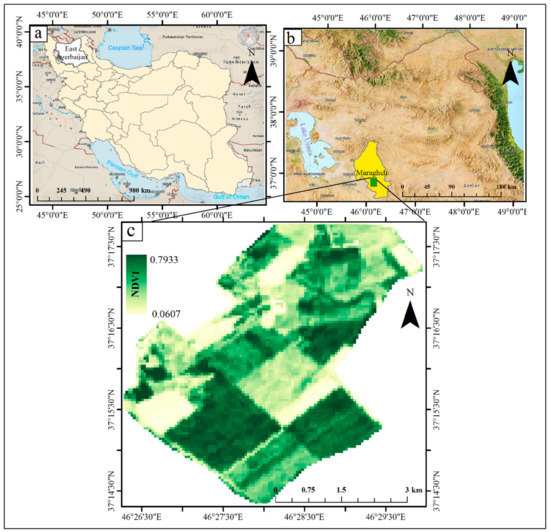
Figure 1.
Location maps of the study site: (a) map of Iran, (b) map of the East Azerbaijan province, (c) the experimental fields operated by Agricultural Research, Education and Extension Organization (AREEO).
2.2. Methodology
Figure 2 shows an overview of the methodology of this study. Accordingly, remotely sensed data in this study consisted of two groups of Sentinel-2 satellite based multispectral data and UAV based RGB images. Besides, line-transect data of the CRC were used as input data for training and validation purposes as the field measurements. To cover the objective of the comparative analysis, two different approaches of fuzzy OBIA and machine learning techniques were applied. In this context, to find the useful method for evaluating the crop residue and tillage intensity, we compared three methods of fuzzy OBIA, ANN and SVM. As shown in Figure 2, construction and running fuzzy OBIA algorithm in the eCognition software environment version 9.1 (Trimble Germany GmbH) included four main steps of the image segmentation, determination of the feature space, selection of the membership function, and classification. Machine learning methods included three steps: training, validation and test. Additional data analysis was carried out for the pixel based ANN and SVM classifications by using ENVI version 5.3 (Exiles Visual Information Solutions, Boulder, Colorado). In order to cover sensitivity analysis of the SVM classifier, four kernels of linear, polynomial, radial basis function (RBF) and sigmoid were applied in the classification process. At the end, the accuracy of the classification methods was evaluated by using four parameters: overall accuracy, Cohen’s kappa, producer accuracy and user accuracy.
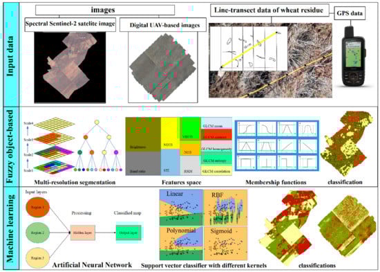
Figure 2.
Overview of the methodology.
2.3. Data Acquisition
Applied remote sensing data in this study included the RGB images (also called color images) from a UAV platform and multispectral images from Sentinel-2 satellite sensor. In this way, a four-rotor UAV named Phantom 3 Professional (SZ DJI Innovations Inc., Shenzhen, China) was used to record high spatial-resolution images after the tillage and planting practices of wheat plants (Figure 3). The UAV was equipped with a 12.4 MP RGB camera supported on a three-axis gimbal. A LiPo 4s battery allowed a maximum flight time of 23 min. The RGB aerial images were recorded with the image size of 4000 × 3000 and ground resolution of about 5 cm at a flight height of 100 m and were saved with the GPS location information. The UAV images were acquired under low wind speed and clear sky conditions between 12:00 am to 00:25 pm and 01:00 pm to 01:25 pm of local time through the total of two individual flights on 5 November 2019.
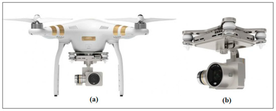
Figure 3.
(a) The unmanned aerial vehicle (UAV) and (b) its built-in digital camera.
The UAV aviated automatically according to the predetermined flight rout to record imagery with nearly 80% forward overlapping and 60% side overlapping which are controlled by the DJI GO mobile application. Following the images from UAV platform are processed by using the software Agisoft Metashape Profession (Agisoft LLC, ST. Petersburg, Russia) to generate an orthoimage. In this way, the key processing steps of image alignment, camera calibration, georeferencing, construction of dense point clouds and generation of the orthoimage were conducted according to the procedure from Lu et al. [60]. Hence, the process of orthomosaic generation with the use of ground control points (GCPs) was carried out in the software environment. Firstly, in order to automatically align the acquired images using a feature point matching algorithm, individual RGB images and GPS data transferred from the camera to the software environment. Secondly, reference coordinates of camera position were used to georeferencing of images and then, the alignment of images had been checked in the total of 12 locations by using ground control points. The camera internal parameters were also estimated by using the image alignment information and reference positions with Brown’s lens distortion model used in Agisoft Metashape [61]. Thirdly, in the build dense cloud dialog box the desired reconstruction parameter of depth filtering had been chosen as mild. It was due to the sharp and small canopy of crop residue [62]. Finally, the digital elevation model (DEM) and orthoimage with a spatial resolution of 5 cm were generated with default parameters and exported as a TIFF image format for subsequent analysis. More detailed information about the orthoimage processing based on Agisoft Metashape software could be seen in [61]. This study was carried out based on the direct use of digital numbers (DN) of orthoimage (see: [48,60,62]).
We downloaded a Sentinel-2 MSI Level-1C (Top-of-Atmosphere reflectance) remotely sensed image acquired on 16 November, 2019 from Copernicus Open Access Hub (https://scihub.copernicus.eu/ (accessed on 2 March 2021)). Table 1 shows the spectral bands of the Sentinel-2 satellite imagery. Atmospheric correction for the imagery was conducted by using the Sen2cor atmospheric correction toolbox in the Sentinel Application Platform (SNAP) software. In order to classify the purposes, totally, the number of ten bands (2–8, 8A, 11 and 12) were clipped to the study area.

Table 1.
Spectral bands of the Sentinel-2 satellite imagery.
2.4. Line-Transect Data
The evaluation of the CRC at the field level is important for validation of the remote sensing data and methods. Field measurements of the CRC are necessary to characterize the applied tillage and planting systems in the fields. Line-transect method is an extensively validated method that is widely used for the measurement of the CRC at the field level and is recommended in the background research [29,33,36,37,42]. In this way, according to the procedure by Wollenhaupt and Pingry [63] we prepared a 30 m long tape and divided it equally into 100 parts. Then, we stretched the tape diagonally to row direction and counted the number of marks that directly were over a piece of crop residue (Figure 4c). Notice that, when counting the marks, sighting was straight down and also only the marks have been counted on which the residue size was not smaller than 0.32 cm (1/8 inch) in diameter. As shown in Figure 4a, line-transect of the CRC performed randomly in the total of 200 locations across the 500 ha of wheat cultivation fields of AREEO to apply for the evaluation of the classification using Sentinel-2 data on 8–19 November 2019. Moreover, the similar operation carried out across 240 ha of wheat cultivation fields of AREEO to measure the CRC in the total of 100 locations (Figure 4b) to apply for the evaluation of the classification using UAV imagery on 20–25 November 2019.
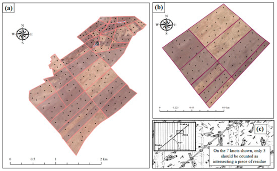
Figure 4.
(a) Distribution of line-transect sampling locations over the study area under Sentinel-2 satellite imagery, (b) Distribution of line transect sampling locations over the study area under UAV imagery, and (c) a close-up of the line-transect method [64].
2.5. Fuzzy OBIA
As indicated in the introduction section, the OBIA is a semiautomated approach that leads to employ variety of spatial, spectral and geometrical features for spatial modelling [43]. The OBIA methodology for the classification of the CRC on the soil surface consists mainly of two successive phases: (a) fixing the boundary of different soil and crop residue compositions by image segmentation and, (b) development of decision rules based on the crop residue characteristics include spectral and textural features which characterize every prepared seedbed as affected by the different tillage and planting practices. In this way, image analysis processes performed using an object-based image analysis program namely, eCognition 9.1 software. In the Section 2.5.1, Section 2.5.2, Section 2.5.3, Section 2.5.4 and Section 2.5.5, applied methods in each phase as well as features selection and model validation are explained in detail.
2.5.1. Image Segmentation
Image segmentation is the first step in OBIA to delineate of the crop residue into the indulgence objects. Despite different methods for splitting up images to homogenous and nonoverlapping regions, multiresolution segmentation is the most common image segmentation algorithm. Technically speaking, it is a bottom-up region-merging algorithm in which adjacent pixels with similar characteristics merge together based on the several user-defined parameters to create initial image objects. Those objects then emerge again according to their similar characteristics to produce larger objects [65,66,67]. Three user-defined parameters (scale, color and shape) control the internal heterogeneity of the produced objects through automatically stopping the process when exceeding thresholds from the defined values. The scale parameter is applied to control the size of the resulting objects. In this context, high values for scale parameter allow high heterogeneity within the image objects and result in larger segments. In contrast, low values for scale parameter increase homogeneity within the image objects and result in smaller segments. In addition, color and shape parameters affect textural and spectral homogeneity of the image objects while shape parameter optimizes the resulting objects through its subparameters: compactness and smoothness [53,68,69].
In this case, due to the application of SWIR bands in the formula of applied tillage indices, we used the bands of Sentinel-2 satellite imagery with the spatial resolution of 20 m include 5, 6, 7, 8A, 11 and 12 in the segmentation process. In the case of UAV imagery, three bands of red, green and blue were included in the segmentation process. The application of trial-and-error method in this study is still a simple and trustworthy method for estimating parameter values [36,70]. Thus, the scale parameters of 4, 5, 6, 7, 8, 9 and 10 tried for the Sentinel-2 satellite image and the scale parameter of 7 represented the best result. In tendency, the scale parameter of 75 obtained for the RGB image from the UAV platform when we tried the scale parameters of 50, 55, 60, 65, 70, 75, 80 and 85. Satellite based and the UAV based images are very different in terms of pixel size. That is why the trusted scale parameters that value for satellite image were very different from that for the RGB orthoimage from the UAV. As a result of this study, defined color and shape factors of 0.7 and 0.3, respectively, provided the most homogeneity within the image objects along with the selected scale parameter (Figure 5).
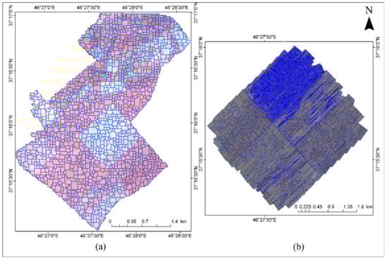
Figure 5.
Multiresolution image segmentation process: (a) the multispectral Sentinel-2 satellite based image, and (b) the RGB image from the UAV.
2.5.2. Fuzzy Rule-Set Based Classification
At the beginning of the fuzzy OBIA classification process, 70 percent of field measurements data were considered as the training data and 30 percent remained for validation of the classification results. After that, training of the OBIA system carried out by demonstrating the following rules: (a) If the values for the CRC within an object become less than 30 percent it assigns to conventional tillage class, (b) If the values for the CRC within an object become 30 percent to 60 percent it assigns to the conservation minimum tillage class, and (c) If the values for the CRC within an object become greater than 60 percent, it assigns to conservation no-tillage class.
2.5.3. Object Based Feature Selection
Feature selection is the most important step for precise assignment of the image objects to the predefined classes [71]. Technically speaking, object-based concept offers the application of new spectral, contextual, textural and geometrical features [72]. Hence, it carried out according to the spectral and textural aspects of the crop residue and soil. Within the research, we aimed to apply and introduce the most efficient object-based features for the CRC which are selected and listed as Table 2.
Table 2.
Applied spectral and textural features space for the fuzzy object based image analysis (OBIA) classification process.
eCognition software is able to conduct the classification procedure either by using the automated nearest neighbor method based on samples or by using the fuzzy membership functions method based on the fuzzy logic theory. Due to the weak performance of the nearest neighbor for identification of different vegetation, soils and crop residue, it seemed not to be much appropriate for the classification of the crop residue cover and tillage intensity [36,52,73]. Hence, the fuzzy membership functions method was chosen to label image objects based on the fuzzy rules. Model design was carried out by using a training/validation dataset process where, firstly, the training sets were used to select the fuzzy membership functions applied to assigning right objects to the right classes and, later, the validation sets were used to evaluate the accuracy of the image classification by calculation of the confusion matrix [74].
2.5.4. Implementation of the Fuzzy Membership Functions
According to Feizizadeh et al. [72] the most important step in an image classification process based on membership functions method is to investigate the qualification of different previously defined features for creation of the classification framework. Thus, from the sample editor window in eCognition software, fuzzy numbers of all features were calculated for each object-class, and then, qualified features with higher fuzzy number values have chosen for each class with respect to predefined classification rules to apply in the classification process. While membership functions are the building blocks of a fuzzy set theory, the shape of applied membership function to calculate the fuzzy number can actually influence a particular fuzzy system. In such a way, among 12 introduced membership functions by eCognition for a wide range of image analysis applications (Figure 6), Gaussian as the most popular membership function because of its simplicity in design and optimization, is continuous and faster for small rule-bases that are mostly advised in previous studies [75]. Hofmann et al. [76] also reported that Gaussian fuzzy membership function is a superior function for classification of a broad range of image objects in particular to vegetative objects. Based on the above-mentioned justifications, we applied Gaussian fuzzy membership function in our study for calculating the fuzzy number of different features of per object-classes to find the qualified features.
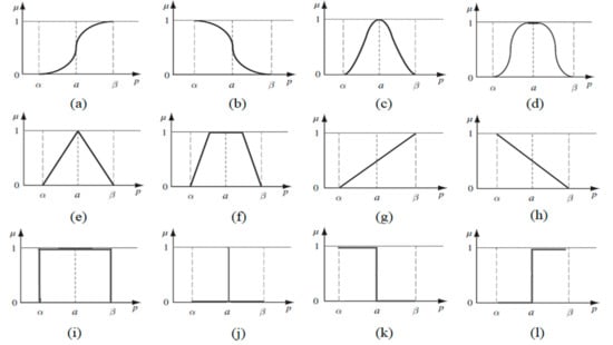
Figure 6.
Typical representatives of fuzzy membership functions with as the describing property and as the degree of membership. Displayed are: (a) larger than, (b) smaller than, (c) Gaussian, (d) about range, (e) linear range (triangle), (f) linear range (triangle inverted), (g) larger than (linear), (h) smaller than (linear), (i) full range, (j) singleton, (k) smaller than (Boolean-crisp), and (l) larger than (Boolean-crisp) [76].
2.5.5. Classification Based on the Fuzzy Operators
Selection of the efficient operator is critical for a fuzzy rule-based classification. To do this, after determination of membership function and identification of the qualified features, a fuzzy logic required to combine these fuzzified features by application of the classification operators [77]. Fuzzy logic in eCognition allows several operators which include “and”, “or”, mean (arithm.) and mean (geom.). Because of the multidimensional conditions by applying different features, it is necessary to use a fuzzy logic on the feature space for combination of the conditions. The simplest and most common operators are “and” and “or” that are also identified as minimum and maximum operators respectively. The operator “and” defined as the default configuration for the image classification and when creating a new class, it combines conditions with the minimum operator. As a result, when the minimum operator (and) is applied, the membership of the output equals the minimum fulfilment of the single statements. Hence, to produce the lowest value of membership and minimize the overlap area between predefined classes, the classification in our study is carried out by using the operator “and”. It also is technically in accordance with [36,40,77].
2.6. Machine Learning Techniques
2.6.1. Artificial Neural Network
The general definition of a neural network model is teaching a system for executing a particular task. A basic neural network model consists of three layers of input layer, hidden layer and output layer [78]. In this method, we defined training classes include intensive tillage, minimum tillage and no-tillage by using the region of interest tool in ENVI 5.3 software. During the classification process, pixel values in the training areas were applied for linking homogenous pixels to the predefined classes [79]. In this context, a feed forward back-propagation network was adopted in a supervised framework. In order to executing applied multilayer perceptron neural network architecture with one hidden layer in this study, neural network parameters were adjusted based on default values in ENVI environment. Eventually, according to a logistic activation mode, training momentum and training threshold contribution parameters were set to 0.9 and 0.9, respectively. In addition, the parameters of training RMS exit criteria, training rate and the number of training iterations were set to 0.1, 0.2 and 100, respectively (for more information see: [80]).
2.6.2. Support Vector Machine
The support vector machines are the set of learning algorithms which are applied for classification of the image pixels/objects [81]. SVMs are supervised nonparametric learning techniques with the ability to produce high classification accuracies. According to the literature, SVMs are not significantly sensitive to the number of training data sets and it makes them be very appealing for the remote sensing applications. In terms of sensitivity analysis, different combinations of configurations of support vector classifier are used for achieving most accuracy in assigning right pixels to the right classes. In this way, a total of four different models were produced and applied for sensitivity analysis of the SVM classifier. SVM used kernels in this study: linear, RBF, sigmoid and polynomial. Gamma in all kernel functions for satellite data was selected as 0.25 and for digital images was selected as 0.33 based on the number of the spectral image bands [82]. Penalty parameter, degree of kernel and bias in the kernel function were considered as default values of 100, 0 and 1 for kernels.
2.7. Accuracy Assessment
The evaluation of classification accuracy essentially determines the quality of the information which is derived from remotely sensed data. Hence, good interpretation of the calculated accuracy parameters from confusion matrix (error matrix) is a very important step to ensure that the desired results are achievable or not [83]. In this context, in addition to overall accuracy and Cohen’s kappa, we considered two other accuracy coefficients of producer accuracy and user accuracy. Applied ground truth data in this study for three classification methods of fuzzy OBIA, ANN and SVM were included in line-transect measurements of the CRC explained in Section 2.4. As mentioned before, line-transect of CRC carried out in the total of 200 locations of the fields under Sentinel-2 satellite imagery and in the 100 total of 100 locations of the fields under UAV imagery. Due to the presence of two phases of learning and validation in image classification using three methods used in this study, 70% of the line-transect data were considered as learning data and the remained 30% applied for validation process in accuracy assessment. Application of truth data for accuracy assessment of fuzzy OBIA in eCognition was based on the creating a training and test area (TTA) mask [84]. Truth data are used as a reference to check classification quality by comparing the classification with reference values (ground truth) based on image objects [69].
According to the procedure by Abbas and Jaber [85] in the case of the pixel-based machine learning image classification in ENVI environment, firstly, polygons containing locations with line-transect of CRC (ground truth data) were introduced on the image as region of interests (ROIs). ROIs consist of three classes: reduce tillage, minimum tillage and no-tillage. Then, ROIs were applied for learning and validation of the image pixels to generate the thematic map of CRC for the study area.
The overall accuracy was calculated by summing the number of correctly classified values and dividing by the total number of values [86] (Equation (1)). The correctly classified values are located along the upper-left to lower-right diagonal of the confusion matrix. The total number of values is the number of values in either the truth or predicted-value arrays [86].
The kappa coefficient measures the agreement between the classification and truth values (Equation (2)) [87]. A kappa value of 1 represents perfect agreement, while a value of 0 represents no agreement [87]. The kappa coefficient is computed as follows:
where is the total number of the classified values compared to the truth values, represents the number of each individual class, is the number of values which belong to the truth class , have also been classified as class , is the total number of truth values belonging to class , and is the total number of predicted values belonging to class . Producer and user accuracies also represented the probability that a value predicted to be in a certain class really is in that class and the probability that a value in a given class was classified correctly, respectively [88].
3. Results
3.1. The Implementation of Fuzzy Space Feature Filters on the Images
Figure 7, Figure 8 and Figure 9 have shown the effects of applying feature space on the images from Sentinel-2 and UAV platforms in order to distinguish different levels of the CRC.
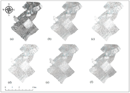
Figure 7.
Applying band ratio feature functions on the Sentinel-2 image: (a) band 5, (b) band 6, (c) band 7, (d) band 8A, (e) band 11 and (f) band 12.
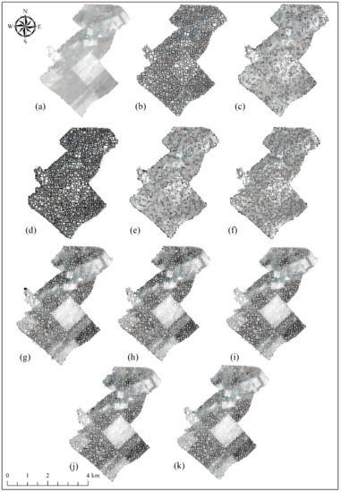
Figure 8.
Applying brightness, GLCM after Haralick and tillage indices feature functions on the Sentinel-2 image: (a) brightness, (b) GLCM contrast, (c) GLCM correlation, (d) GLCM homogeneity, (e) GLCM entropy, (f) GLCM mean, (g) NDTI, (h) STI, (i) NITI, (j) RSDI, and (k) VRETI.
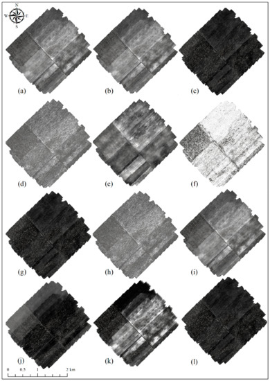
Figure 9.
Application of features functions on the mosaicked UAV images: (a) red, (b) green, (c) blue, (d) Std.Dev red, (e) Std.Dev green, (f) brightness, (g) Std.Dev blue, (h) GLCM correlation, (i) GLCM homogeneity, (j) GLCM contrast, (k) GLCM mean, and (l) GLCM entropy.
3.2. Fuzzy OBIA Classification
Before the classification process, firstly, the process of mosaicking was conducted on the RGB images from the UAV in order to obtain an orthoimage that it covers the whole study area, and later, the process of segmentation carried out to achieve the image objects with the similar-attributes pixels. After that the selection or features were performed based on spectral properties of the digital images. In this way, because digital UAV based images consist of three bands of red, green and blue, the features have only been used for the application in the fuzzy membership process that were a function of those three bands. Therefore, tillage and vegetation indices were not included in the features space. Table 3 shows the results of calculation of the fuzzy numbers for the features space per object classes.
Table 3.
Fuzzy numbers for different features about three classes of tillage intensity for the digital UAV image.
By using the results of Table 3, the features with high degree of membership derived as input variables for the classification step. The final selection of the features space for the image classification was in such a way that the average of the selected features values did not differ significantly from the feature with the maximum value of degree of membership. It was due to the probable error from features with low membership value that could influence classification accuracy [71,77]. In this context, the number of contributed features in the final classification process depended on their effects for maximizing classification accuracy about each individual class. Thus, firstly, the features with highest degree of membership for each class were added gradually to the final feature space. Then, classification accuracy for each class was evaluated individually. Finally, including additional features in the classification feature space continued as long as the classification accuracy from contributing the last item reduced the classification accuracy [71,72,89]. Consequently, after the selection of different combinations of the features space and evaluation of the classification results for the UAV images, it was observed that the most efficient combination for objects-class of intensive tillage consisted five features of brightness, average of red and green band values (band ratio) and GLCM homogeneity and GLCM mean (textural features). It was a bit different for minimum tillage objects-class where the selected features only included the group of band ratio indicators which consisted four indicators of blue, green, red and brightness in addition to GLCM mean. The third objects-class was no-tillage that went through trial of the different combination of the features space and in contrast with two previous classes, Std.Dev bands values were very useful in assigning right objects to the no-tillage class. Finally, the combination of the Std.Dev features with red band and brightness (band ratio) as well as GLCM contrast and GLCM homogeneity represented the most accuracy in the result.
Sentinel-2 features selection was carried out after producing objects with homogenous pixels by the image segmentation process. As previously mentioned in the part of Section 2.5.3, in total we considered nineteen spectral and textural attributes as features space. In this context, Gaussian membership function applied on the features space and lastly, features with highest fuzzy numbers were selected for being used as input variables when the combination of features using operator “and” taking place in the image classification step. Table 4 has shown fuzzy membership values for features space per objects-classes.
Table 4.
Fuzzy numbers for different features about three classes of tillage intensity for multispectral Sentinel-2 satellite image.
Trial of different combinations of the features performed to achieve features space in which the highest value obtained for accuracy of the image classification. In this way, firstly, the qualified combination for intensive tillage objects-class consisted two band ratio indicators of band 11 and band 12, two tillage indicators of NDTI and STI and three textural features of GLCM correlation, GLCM mean and GLCM contrast. Later, the qualified combination of the features space for assigning right objects to the minimum tillage class included five spectral and textural features of band 12, NDTI, STI, GLCM correlation, and GLCM homogeneity. In addition, the most acceptable features space for the third class was a composition of seven features of band 11, band 12, brightness, NDTI, STI, GLCM mean and GLCM correlation. The capability of the tillage indices to make difference between residue and soil background as well as the efficiency of the bands of 11 and 12 in performed trials for classes of minimum tillage and no-tillage where levels of the CRC on the soil surface were more than 30 percent clearly verified particular behavior of the spectral signature of the crop residue near 2100 nm. Our findings are in accordance with [36,53].
After a thorough investigation of different features to find the most useful features space, automated image classification carried out using operator “and” which combines features with the minimum operator. Later, the evaluation of classification accuracy of two used platforms performed using confusion matrix. In this way, we considered the number of 100 and 200 which measured points of the CRC from line-transect method in order to validation of the digital UAV and the multispectral Sentinel-2 images classification. The reason for fewer validation points for UAV image is because of covering the smaller area by the UAV image due to the application costs. Table 5 indicated the results of Evaluation of the Fuzzy OBIA method of Classification for the both of UAV and Sentinel-2 platforms.
Table 5.
Evaluation of the Fuzzy OBIA method of the classification for the both of UAV and Sentinel-2 platforms using confusion matrix.
In general, overall accuracy and Cohen’s kappa are two main parameters for the evaluation of the accuracy of an image classification process [90]. Overall accuracy that is the sum of the number of correctly classified objects which are divided by the total number of validation points [85] was 0.880 and 0.920 for the classification of the CRC and tillage intensity by using digital UAV based and multispectral Sentinel-2 satellite images, respectively. Despite the higher spatial resolution of the UAV based image, it is observed that image objects containing a mixture of soil and CRC are better-assigned to the predefined classes. As previously mentioned, spectral signatures of soil and crop residue have absorption properties in shortwave infrared area of the electromagnetic spectrum. That is why tillage indices use the absorption properties of the region near 2100 nm. As a result, the use of Sentinel-2 image enables us to include spectral indices in features space of the image classification and it is the key for detection of the crop residue with higher accuracy. Therefore, it can be concluded that spectral resolution is the most important factor in identification of the CRC. We also obtained Cohen’s kappa of 0.811 and 0.874 for the UAV and the Sentinel-2 platforms, respectively. As previously mentioned, it can range from 0 to 1 where 0 represents that there is random agreement between raters and 1 represents perfect agreement among the raters.
User accuracy is a very important scale for a final user to know the probability that an image object predicted to be in a certain class really is in that class. We found that the most incorrectly classified objects belong to the minimum tillage class. Producer accuracy is the probability that an image object in a given class was classified correctly. In this way, we observed that the most correctly classified objects belong to no-tillage class for the both UAV and Sentinel-2. The maximum errors are from the minimum tillage class about the both UAV and Sentinel-2 images. It can be due to the effect of intermixture of the objects from two other classes in the boundaries of predefined threshold for minimum tillage. So, we found that there is a clear contrast between intensive tillage and no tillage, but it is not being verified when considering no tillage and minimum tillage or intensive tillage and minimum tillage. Accordingly, the classifier assigned the majority of the image objects that were a mixture of soil and more than 85 percent of the crop residue to the right no-tillage class about the both UAV and Sentinel-2 images.
3.3. Neural Network Classification
Analysis of the agricultural study area of AREEO by using neural network classification approach which is carried out in ENVI 5.3 environment. Firstly, a number of three types of the tillage and planting practices classes include intensive tillage (light brown), Minimum tillage (green) and no-tillage (yellow) which are established for the classification of images pixels. Secondly, we clustered line-transect measurements of the CRC into the preset classes and enter those in neural network model as training data. Table 6 has shown the evaluation of the neural network method of classification for the both of UAV and Sentinel-2 platforms.
Table 6.
Results of neural network classification for the digital images from UAV and spectral image from Sentinel-2 satellite.
3.4. Support Vector Machine Classification
Here, image classification processes are performed with the SVMs classifiers. As discussed in Section 2.6.2, four SVM kernels were used for the classification of the tillage and planting practices in the three classes of intensive tillage, minimum tillage and no-tillage. Classification results of different SVMs are shown in Table 7.
Table 7.
Results of pixel-based SVM classifications algorithms with different kernels for the digital images from the UAV and spectral image from Sentinel-2 satellite.
According to the results of Table 7, well-known SVM RBF kernel surpassed other three kernels to assign right pixels to the right classes.
Graphical display of the performed tillage and planting practices based on different classification approaches for multispectral Sentinel-2 and digital UAV images are shown in Figure 10 and Figure 11.
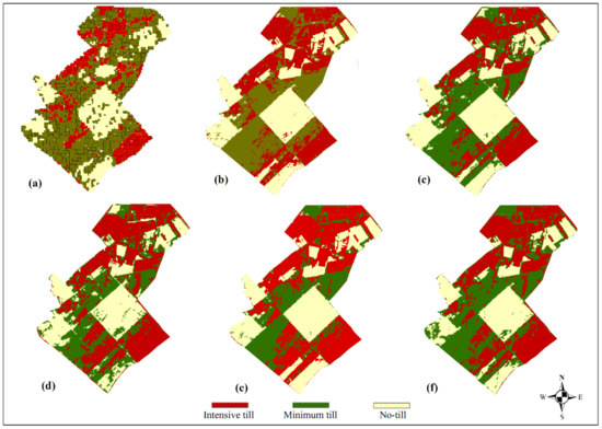
Figure 10.
Classification maps of the tillage and planting practices for the Sentinel-2 multispectral image: (a) fuzzy OBIA, (b) ANN, (c) SVM (RBF), (d) SVM (polynomial), (e) SVM (linear) and (f) SVM (sigmoid).
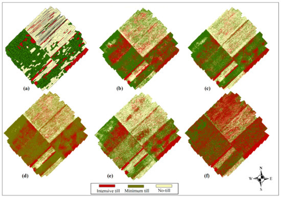
Figure 11.
Classification maps of the tillage and planting practices for the digital UAV based on the images: (a) fuzzy OBIA, (b) ANN, (c) SVM (RBF), (d) SVM (polynomial), (e) SVM (linear), and (f) SVM (sigmoid).
4. Discussion
Recent progress in remote sensing and earth observation technologies highlighted the significance of the automated/semiautomated methods as quick and effective data is driven the approach in the remote seining domain. Thus, development of the automated or semiautomated methods of evaluation is essential for the analysis of big data in remote sensing. In spite of the development of different remote sensing platforms with different spatial and spectral characteristics, the use of learning based methods for analysis of the input data is inevitable. By these means, we analyzed two types of imagery based on two different image analysis approaches of semiautomated fuzzy object-based and machine learning methods to detect the amount of the CRC left on the soil surface after the tillage and planting processes. It helps in identifying tillage intensity of applied practices during the seedbed preparation operations.
According to the literatures, fuzzy OBIA has a critical advantage over pixel-based methods of the image classification [50,54,76]. It is the utilization of the spectral, textural, shape and size properties in addition to the brightness of the image objects in the classification process [36,40,77]. We found that Tillage indices were a major part of utilized spectral properties in this study that improved the classification accuracy of fuzzy OBIA against two other methods. Based on the findings from Serbin et al. [26] and Daughtry et al. [27,28] it was due to the absorption properties of the electromagnetic spectrum near 2100 nm which is caused by C-O and O-H bonds from lignin and cellulose and other saccharides in the external wall of the crop residue. This characteristic makes those instantly recognizable by using correspondence spectral indices NDTI and STI in which the area around 2100 nm is covered by spectral used bandwidths. Hence, Figure 7 shows a clear contrast between the CRC and soil when applying NDTI and STI filters on the Sentinel-2 satellite image that also was in accordance with Najafi et al. [53]. In contrast, the only factor for distinguishing image pixels in the two machine learning methods (SVM and ANN) was the brightness of image pixels.
We also observed that, in spite of the high spatial resolution of the RGB images from the UAV platform than the multispectral Sentinel-2 based image, accuracies are greater in the classification of the Sentinel-2 image when applying fuzzy OBIA method. It proves the effectiveness of the spectral tillage indices in the classification of the Sentinel-2 image by using fuzzy OBIA method. The RGB images due to the lack of NIR and SWIR bands are not able to use spectral indices in their feature space. Our finding is supported by the drawn results from García-Martínez et al [91] who estimated canopy cover by using RGB and multispectral imagery.
As reported by Pan et al. [49] on the formation of salt and pepper effects in pixel-based analysis of very high-resolution images we also observed this effect when applying the pixel based SVM and ANN methods of the image classification. It led to the formation of a heterogeneous mixture of different classes in each class in the final classification map. Thus, increasing this type of entropy in the field scale not only does not help in the interpretation of the results but also it leads to a confused final user. Segmentation process in the fuzzy OBIA method of the classification through the merge of adjacent pixels with similar characteristics and formation of image objects minimized those errors during classification.
Classification results of the application of the SVM and NN methods showed that Sentinel-2 image has slight superiority for assigning image pixels to the right classes in comparison with UAV. It was due to the fact that, in spite of the higher spatial resolution of the UAV image, soil background effects were considered as disturbance factors in the classification of the RGB orthoimage from UAV [92]. It also observed that those effects reached to the highest value when applying the SVM classifier with linear kernel. In addition, the effects of mixing of pixels especially at class boundaries reduced classification accuracy.
One of the limitations with fuzzy OBIA was that this method needs experts with scientific and practical information about the relationship between the spectral properties and the CRC for the selection of correct features space [71], but that information is unnecessary in the classification by using the SVM and ANN methods. This also could be a motivation factor for wide application of the fuzzy OBIA classification method for the evaluation of the CRC and tillage intensity to reach more accurate results. The efficiency of fuzzy OBIA has been recently addressed by researchers [93,94,95,96] while acknowledging the significance of this integrated approach as an optimized semiautomated object based classification technique.
5. Conclusions and Future Work
Conservation tillage methods through leaving the previous CRC on the soil surface protect it from water and wind erosions. Here we considered a comparative approach for a novel fuzzy OBIA method and common pixel-based machine learning methods for the estimation of the CRC from previous cultivated winter wheat after the tillage and planting practices. Applied remote sensing data in this study consisted of RGB images from UAV and multispectral images from Sentinel-2 satellite. Based on the results, we concluded that the fuzzy OBIA based on Gaussian membership function represented efficient results for the classification of the CRC. In spite of superior spatial resolution in RGB orthoimage from UAV, it is observed that overall classification accuracy for Sentinel-2 data surpassed the UAV images. For the multispectral Sentinel-2 image the combination include four features of band 12, NDTI, STI and GLCM correlation represented acceptable fuzzy numbers and maximized the classification accuracy across three classes of CRC. For the classification of UAV orthoimage the combination of the brightness, red, green, GLCM homogeneity and GLCM mean maximized the differences between soil and residue for the intensive tillage class. In addition, the features of blue, green, red and GLCM mean for minimum tillage class and Std.Dev of three bands of red, blue and green along with the brightness, GLCM contrast and GLCM homogeneity represented the highest classification accuracy. Implementation of SVM and ANN algorithms indicated that in spite of the capability of the SVM classifier with the RBF kernel and also the ANN classifier to the classification of different tillage methods based on the CRC, these methods are turned not to be as efficient as the fuzzy OBIA classifier for estimating the CRC. Based on the results of the current research, our future research will focus and apply an integrated approach of deep learning and fuzzy OBIA for monitoring the trend of the CRC and its impacts on conservation of soil. From the methodological perspective, it is widely known that the recent progress in remote sensing technology makes available satellite images with improved spectral and spatial properties. Thus, proposing and applying efficient and automated data of driven approach such as fuzzy OBIA or machine learning techniques (SVM, ANN) will support future researchers to identify the robust and weakness of each method. Based on this statement, the results of the current research can be considered as the progressive research in the domain of remote sensing science.
Author Contributions
Conceptualization, H.N., P.N., and B.F.; Methodology, B.F. and P.N.; Software, P.N. and B.F.; Validation, P.N.; Formal Analysis, P.N.; Investigation, H.N. and B.F.; Resources, H.N., B.F., and P.N; Data Curation, P.N.; Writing—Original Draft Preparation, P.N.; Writing—Review and Editing, P.N., B.F. and H.N.; Visualization, P.N.; Supervision, P.N., H.N. and B.F; Project Administration, H.N. and B.F.; Funding Acquisition, H.N. and B.F. All authors have read and agreed to the published version of the manuscript.
Funding
This research received no external funding.
Institutional Review Board Statement
Not applicable.
Informed Consent Statement
Not applicable.
Data Availability Statement
Data will be available by request.
Acknowledgments
This research is supported by a research grant from the University of Tabriz (number v/d/1692).
Conflicts of Interest
The authors declare no conflict of interest.
References
- Kopittke, P.M.; Menzies, N.W.; Wang, P.; McKenna, B.A.; Lombi, E. Soil and the intensification of agriculture for global food security. Environ. Int. 2019, 132, 105078. [Google Scholar] [CrossRef] [PubMed]
- Noel, S. Economics of Land Degradation Initiative: Report for policy and decision makers_ Reaping Economic and Environmental Benefits from Sustainable Land Managemen; Economics of Land Degradation (ELD) Initiative: Bonn, Germany, 2016. [Google Scholar]
- Status of the World’s Soils; Food and Agriculture Organization of the United Nations and Intergovernmental Technical Panel on Soils: Rome, Italy, 2015.
- Bryant, C.J.; Krutz, L.J.; Reynolds, D.B.; Locke, M.A.; Golden, B.R.; Irby, T.; Steinriede, R.W., Jr.; Spencer, G.D.; Mills, B.E.; Wood, C.W. Conservation soybean production systems in the mid-southern USA: I. Transitioning from conventional to conservation tillage. Crop. Forage Turfgrass Manag. 2020, 6, e20055. [Google Scholar] [CrossRef]
- Torabian, S.; Farhangi-Abriz, S.; Denton, M.D. Do tillage systems influence nitrogen fixation in legumes? A review. Soil Till. Res. 2019, 185, 113–121. [Google Scholar] [CrossRef]
- Shahzad, M.; Hussain, M.; Farooq, M.; Farooq, S.; Jabran, K.; Nawaz, A. Economic assessment of conventional and conservation tillage practices in different wheat-based cropping systems of Punjab, Pakistan. Environ. Sci. Pollut. Res. 2017, 24, 24634–24643. [Google Scholar] [CrossRef]
- Rahmati, M.; Eskandari, I.; Kouselou, M.; Feiziasl, V.; Mahdavinia, G.R.; Aliasgharzad, N.; McKenzie, B.M. Changes in soil organic carbon fractions and residence time five years after implementing conventional and conservation tillage practices. Soil Till. Res. 2020, 200, 104632. [Google Scholar] [CrossRef]
- Jia, L.; Zhao, W.; Zhai, R.; Liu, Y.; Kang, M.; Zhang, X. Regional differences in the soil and water conservation efficiency of conservation tillage in China. Catena 2019, 175, 18–26. [Google Scholar] [CrossRef]
- Larney, F.J.; Lindwall, C.W.; Izaurralde, R.C.; Moulin, A.P. Tillage systems for soil and water conservation on the Canadian prairie. In Conservation Tillage in Temperate Agroecosystems; CRC Press, Tailor & Francis: Boca Raton, FL, USA, 2017; pp. 305–328. [Google Scholar]
- Endale, D.M.; Schomberg, H.H.; Truman, C.C.; Franklin, D.H.; Tazisong, I.A.; Jenkins, M.B.; Fisher, D.S. Runoff and nutrient losses from conventional and conservation tillage systems during fixed and variable rate rainfall simulation. J. Soil Water Conserv. 2019, 74, 594–612. [Google Scholar] [CrossRef]
- Lampurlanés, J.; Plaza-Bonilla, D.; Álvaro-Fuentes, J.; Cantero-Martínez, C. Long-term analysis of soil water conservation and crop yield under different tillage systems in Mediterranean rainfed conditions. Field Crops Res. 2016, 189, 59–67. [Google Scholar] [CrossRef]
- CTIC. Tillage Type Definitions. West Lafayette, In Conservation Technology Information Center. 2002. Available online: https://www.ctic.org/resource_display/?id=322 (accessed on 8 November 2020).
- Mitchell, J.P. Classification of Conservation Tillage Practices in California Irrigated Row Crop Systems; UC ANR Publication 8364; UC ANR Publication: Oakland, CA, USA, 2009. [Google Scholar]
- Goddard, T.; Zoebisch, M.; Gan, Y.; Ellis, W.; Watson, A.; Sombatpanit, S. No-Till Farming Systems; World Association of Soil and Water Conservation: Bangkok, Thailand, 2008. [Google Scholar]
- Laflen, J.M.; Amemiya, M.; Hintz, E.A. Measuring crop residue cover. J. Soil Water Conserv. 1981, 36, 341–343. [Google Scholar]
- NRCS. Farming with Crop Residue. 1992. Available online: https://www.nrcs.usda.gov/wps/portal/nrcs/detail/national/technical/nra/rca/?cid=nrcs144p2_027241 (accessed on 2 March 2021).
- Laamrani, A.; Pardo Lara, R.; Berg, A.A.; Branson, D.; Joosse, P. Using a mobile device “app” and proximal remote sensing technologies to assess soil cover fractions on agricultural fields. Sensors 2018, 18, 708. [Google Scholar] [CrossRef] [PubMed]
- Laamrani, A.; Joosse, P.; Feisthauer, N. Determining the number of measurements required to estimate crop residue cover by different methods. J. Soil Water Conserv. 2017, 72, 471–479. [Google Scholar] [CrossRef]
- Beeson, P.C.; Daughtry, C.S.; Hunt, E.R.; Akhmedov, B.; Sadeghi, A.M.; Karlen, D.L.; Tomer, M.D. Multispectral satellite mapping of crop residue cover and tillage intensity in Iowa. J. Soil Water Conserv. 2016, 71, 385–395. [Google Scholar] [CrossRef]
- Najafi, P.; Navid, H.; Feizizadeh, B.; Eskandari, I. Remote sensing for crop residue cover recognition: A review. Agric. Eng. Int. CIGR J. 2018, 20, 63–69. [Google Scholar]
- Tenkorang, F.; Lowenberg-DeBoer, J. On-farm profitability of remote sensing in agriculture. J. Terr. Obs. 2008, 1, 6. [Google Scholar]
- Wang, T.; Thomasson, J.A.; Yang, C.; Isakeit, T.; Nichols, R.L.; Collett, R.M.; Han, X.; Bagnall, C. Unmanned aerial vehicle remote sensing to delineate cotton root rot. J. Appl. Remote Sens. 2020, 14, 034522. [Google Scholar] [CrossRef]
- Cai, W.; Zhao, S.; Wang, Y.; Peng, F.; Heo, J.; Duan, Z. Estimation of winter wheat residue coverage using optical and SAR remote sensing images. Remote Sens. 2019, 11, 1163. [Google Scholar] [CrossRef]
- Li, Z.; Guo, X. Remote sensing of terrestrial non-photosynthetic vegetation using hyperspectral, multispectral, SAR, and LiDAR data. Prog. Phys. Geogr. 2016, 40, 276–304. [Google Scholar] [CrossRef]
- Thoma, D.P.; Gupta, S.C.; Bauer, M.E. Evaluation of optical remote sensing models for crop residue cover assessment. J. Soil Water Conserv. 2004, 59, 224–233. [Google Scholar]
- Serbin, G.; Daughtry, C.S.; Hunt, E.R., Jr.; Reeves, J.B., III; Brown, D.J. Effects of soil composition and mineralogy on remote sensing of crop residue cover. Remote Sens. Environ. 2009, 113, 224–238. [Google Scholar] [CrossRef]
- Daughtry, C.S.T.; Hunt, E.R., Jr. Mitigating the effects of soil and residue water contents on remotely sensed estimates of crop residue cover. Remote Sens. Environ. 2008, 112, 1647–1657. [Google Scholar] [CrossRef]
- Daughtry, C.S.; Doraiswamy, P.C.; Hunt, E.R., Jr.; Stern, A.J.; McMurtrey, J.E., III; Prueger, J.H. Remote sensing of crop residue cover and soil tillage intensity. Soil Till. Res. 2006, 91, 101–108. [Google Scholar] [CrossRef]
- Zheng, B.; Campbell, J.B.; de Beurs, K.M. Remote sensing of crop residue cover using multi-temporal Landsat imagery. Remote Sens. Environ. 2012, 117, 177–183. [Google Scholar] [CrossRef]
- Quemada, M.; Daughtry, C.S. Spectral indices to improve crop residue cover estimation under varying moisture conditions. Remote Sens. 2016, 8, 660. [Google Scholar] [CrossRef]
- Yue, J.; Tian, Q. Estimating fractional cover of crop, crop residue, and soil in cropland using broadband remote sensing data and machine learning. Int. J. Appl. Earth Obs. Geoinf. 2020, 89, 102089. [Google Scholar] [CrossRef]
- Raoufat, M.H.; Dehghani, M.; Abdolabbas, J.; Kazemeini, S.A.; Nazemossadat, M.J. Feasibility of satellite and drone images for monitoring soil residue cover. J. Saudi Soc. Agric. Sci. 2020, 19, 56–64. [Google Scholar]
- Serbin, G.; Hunt, E.R.; Daughtry, C.S.T.; McCarty, G.W.; Doraiswamy, P.C. An improved ASTER index for remote sensing of crop residue. Remote Sens. 2009, 1, 971–991. [Google Scholar] [CrossRef]
- McNairn, H.; Protz, R. Mapping corn residue cover on agricultural fields in Oxford County, Ontario, using Thematic Mapper. Can. J. Remote Sens. 1993, 19, 152–159. [Google Scholar] [CrossRef]
- Van Deventer, A.P.; Ward, A.D.; Gowda, P.H.; Lyon, J.G. Using Thematic Mapper data to identify contrasting soil plains and tillage practices. Photogram. Eng. Remote Sens. 1997, 63, 87–93. [Google Scholar]
- Najafi, P.; Navid, H.; Feizizadeh, B.; Eskandari, I.; Blaschke, T. Fuzzy object-based image analysis methods using Sentinel-2A and Landsat-8 data to map and characterize soil surface residue. Remote Sens. 2019, 11, 2583. [Google Scholar] [CrossRef]
- Daughtry, C.S.T.; Hunt, E.R.; Doraiswamy, P.C.; McMurtrey, J.E. Remote sensing the spatial distribution of crop residues. Agron. J. 2005, 97, 864–871. [Google Scholar] [CrossRef]
- Böhler, J.E.; Schaepman, M.E.; Kneubühler, M. Optimal timing assessment for crop separation using multispectral unmanned aerial vehicle (UAV) data and textural features. Remote Sens. 2019, 11, 1780. [Google Scholar]
- Huang, X.; Zhang, L.; Wang, L. Evaluation of morphological texture features for mangrove forest mapping and species discrimination using multispectral IKONOS imagery. IEEE Geosci. Remote. Sens. Lett. 2009, 6, 393–397. [Google Scholar] [CrossRef]
- Kim, H.O.; Yeom, J.M. Effect of red-edge and texture features for object-based paddy rice crop classification using RapidEye multi-spectral satellite image data. Int. J. Remote Sens. 2014, 35, 7046–7068. [Google Scholar] [CrossRef]
- Peña-Barragán, J.M.; Ngugi, M.K.; Plant, R.E.; Six, J. Object-based crop identification using multiple vegetation indices, textural features and crop phenology. Remote Sens. Environ. 2011, 115, 1301–1316. [Google Scholar] [CrossRef]
- Jin, X.; Ma, J.; Wen, Z.; Song, K. Estimation of maize residue cover using Landsat-8 OLI image spectral information and textural features. Remote Sens. 2015, 7, 14559–14575. [Google Scholar] [CrossRef]
- Blaschke, T.; Feizizadeh, B.; Hölbling, D. Object-based image analysis and digital terrain analysis for locating landslides in the Urmia Lake Basin, Iran. IEEE J. Sel. Top. Appl. Earth Obs. Remote Sens. 2014, 7, 4806–4817. [Google Scholar] [CrossRef]
- Duro, D.C.; Franklin, S.E.; Dubé, M.G. A comparison of pixel-based and object-based image analysis with selected machine learning algorithms for the classification of agricultural landscapes using SPOT-5 HRG imagery. Remote Sens. Environ. 2012, 118, 259–272. [Google Scholar] [CrossRef]
- Kim, H.O.; Yeom, J.M. A study on object-based image analysis methods for land cover classification in agricultural areas. J. Korean Assoc. Geogr. Inf. Stud. 2012, 15, 26–41. [Google Scholar] [CrossRef][Green Version]
- Huang, H.; Lan, Y.; Yang, A.; Zhang, Y.; Wen, S.; Deng, J. Deep learning versus Object-based Image Analysis (OBIA) in weed mapping of UAV imagery. Int. J. Remote Sens. 2020, 41, 3446–3479. [Google Scholar] [CrossRef]
- David, L.C.G.; Ballado, A.H. Vegetation indices and textures in object-based weed detection from UAV imagery. In Proceedings of the 2016 6th IEEE International Conference on Control System, Computing and Engineering (ICCSCE), Batu Ferringhi, Malaysia, 25–27 November 2016; pp. 273–278. [Google Scholar]
- Sumesh, K.C.; Ninsawat, S.; Som-ard, J. Integration of RGB-based vegetation index, crop surface model and object-based image analysis approach for sugarcane yield estimation using unmanned aerial vehicle. Comput. Electron Agric. 2021, 180, 105903. [Google Scholar]
- Pan, G.; Li, F.M.; Sun, G.J. Digital camera based measurement of crop cover for wheat yield prediction. In Proceedings of the 2007 IEEE International Geoscience and Remote Sensing Symposium, Barcelona, Spain, 23–28 July 2007; pp. 797–800. [Google Scholar]
- Blaschke, T.; Hay, G.J.; Kelly, M.; Lang, S.; Hofmann, P.; Addink, E.; Feitosa, R.; van der Meer, F.; van der Werff, H.; van Coillie, F.; et al. Geographic Object-based Image Analysis: A new paradigm in Remote Sensing and Geographic Information Science. ISPRS J. Photogramm. Remote Sens. 2014, 87, 180–191. [Google Scholar] [CrossRef] [PubMed]
- Kalantar, B.; Mansor, S.B.; Sameen, M.I.; Pradhan, B.; Shafri, H.Z. Drone-based land-cover mapping using a fuzzy unordered rule induction algorithm integrated into object-based image analysis. Int. J. Remote Sens. 2017, 38, 2535–2556. [Google Scholar] [CrossRef]
- Bauer, T.; Strauss, P.A. Rule-based image analysis approach for calculating residues and vegetation cover under field conditions. Catena 2014, 113, 363–369. [Google Scholar] [CrossRef]
- Najafi, P.; Navid, H.; Feizizadeh, B.; Eskandari, I. Object-based satellite image analysis applied for crop residue estimating using Landsat OLI imagery. Int. J. Remote Sens. 2018, 39, 6117–6136. [Google Scholar] [CrossRef]
- Hossain, M.D.; Chen, D. Segmentation for Object-Based Image Analysis (OBIA): A review of algorithms and challenges from remote sensing perspective. ISPRS J. Photogramm. Remote Sens. 2019, 150, 115–134. [Google Scholar] [CrossRef]
- Bocco, M.; Sayago, S.; Willington, E. Neural network and crop residue index multiband models for estimating crop residue cover from Landsat TM and ETM+ images. Int. J. Remote Sens. 2014, 35, 3651–3663. [Google Scholar] [CrossRef]
- Sudheer, K.P.; Gowda, P.; Chaubey, I.; Howell, T. Artificial neural network approach for mapping contrasting tillage practices. Remote Sens. 2010, 2, 579–590. [Google Scholar] [CrossRef]
- Beck, H.E.; Zimmermann, N.E.; McVicar, T.R.; Vergopolan, N.; Berg, A.; Wood, E.F. Present and future Köppen-Geiger climate classification maps at 1-km resolution. Sci. Data. 2018, 5, 180214. [Google Scholar] [CrossRef] [PubMed]
- IMO (Iran Meteorological Organization). General Meteorological Department of East Azerbaijan Province. 2018. Available online: http://eamo.ir/Stats-and-Infos/Yearly.aspx (accessed on 1 March 2021).
- Soil Survey Staff. Soil Taxonomy: A Basic System of Soil Classification for Making and Interpreting Soil Surveys, 2nd ed.; U.S. Gov. Print: Washington, DC, USA, 1999.
- Lu, N.; Zhou, J.; Han, Z.; Li, D.; Cao, Q.; Yao, X.; Tian, Y.; Zhu, Y.; Cao, W.; Cheng, T. Improved estimation of aboveground biomass in wheat from RGB imagery and point cloud data acquired with a low-cost unmanned aerial vehicle system. Plant Methods 2019, 15, 17. [Google Scholar] [CrossRef] [PubMed]
- Agisoft, L.L.C. Agisoft Metashape User Manual, Professional Edition, Version 1.7; Agisoft LLC, St.: Petersburg, Russia, 2021; Available online: https://www.agisoft.com/pdf/metashape-pro_1_7_en.pdf (accessed on 5 January 2021).
- Li, S.; Yuan, F.; Ata-UI-Karim, S.T.; Zheng, H.; Cheng, T.; Liu, X.; Tian, Y.; Zhu, Y.; Cao, W.; Cao, Q. Combining color indices and textures of UAV-based digital imagery for rice LAI estimation. Remote Sens. 2019, 11, 1763. [Google Scholar] [CrossRef]
- Wollenhaupt, N.C.; Pingry, J. Estimating Residue Using the Line Transect Method; University of Wisconsin—Extension: Madison, WI, USA, 1991. [Google Scholar]
- Eck, K.J.; Brown, D.E. Estimating Corn and Soybean Residue Cover. Agronomy Guide. West Lafayette, Indiana 47907. Purdue University Cooperative Extension Service. SOILS (TILLAGE). AY-269-W. Available online: https://www.extension.purdue.edu/extmedia/AY/AY-269-W.pdf (accessed on 2 March 2021).
- Baatz, M. Multi resolution segmentation: An optimum approach for high quality multi scale image segmentation. In Beutrage zum AGIT-Symposium; Salzburg: Heidelberg, Germany, 2000; pp. 12–23. [Google Scholar]
- Rahman, M.R.; Saha, S.K. Multi-resolution segmentation for object-based classification and accuracy assessment of land use/land cover classification using remotely sensed data. J. Indian Soc. Remote Sens. 2008, 36, 189–201. [Google Scholar] [CrossRef]
- Happ, P.N.; Ferreira, R.S.; Bentes, C.; Costa, G.A.O.P.; Feitosa, R.Q. Multiresolution segmentation: A parallel approach for high resolution image segmentation in multicore architectures. The International Archives of the Photogrammetry. Remote Sens. Spat. Inf. Sci. 2010, 38, C7. [Google Scholar]
- Blaschke, T.; Burnett, C.; Pekkarinen, A. Remote Sensing Image Analysis: Including the Spatial Domain Image segmentation methods for object-based analysis and classification. In Remote Sensing and Digital Image Processing; Jong, S.M.D., Meer, F.D.V., Eds.; Springer: Dordrecht, Germany, 2004; pp. 211–236. [Google Scholar]
- Feizizadeh, B.; Blaschke, T. A semi-automated object based image analysis approach for landslide delineation. In Proceedings of the European Space Agency Living Planet Symposium, Edinburgh, UK, 9–13 September 2013; pp. 9–13. [Google Scholar]
- Tong, H.; Maxwell, T.; Zhang, Y.; Dey, V. A supervised and fuzzy-based approach to determine optimal multi-resolution image segmentation parameters. Photogramm. Eng. Remote Sens. 2012, 78, 1029–1044. [Google Scholar] [CrossRef]
- Feizizadeh, B. A novel approach of fuzzy dempster–shafer theory for spatial uncertainty analysis and accuracy assessment of object-based image classification. IEEE Geosci. Remote. Sens. Lett. 2017, 15, 18–22. [Google Scholar] [CrossRef]
- Feizizadeh, B.; Blaschke, T.; Tiede, D.; Moghaddam, M.H.R. Evaluating fuzzy operators of an object-based image analysis for detecting landslides and their changes. Geomorphology 2017, 293, 240–254. [Google Scholar] [CrossRef]
- Zabala, A.; Cea, C.; Pons, X. Segmentation and thematic classification of color orthophotos over non-compressed and JPEG 2000 compressed images. Int. J. Appl. Earth Obs. Geoinf. 2012, 15, 92–104. [Google Scholar] [CrossRef]
- Wright, C.; Gallant, A. Improved wetland remote sensing in Yellowstone National Park using classification trees to combine TM imagery and ancillary environmental data. Remote Sens. Environ. 2007, 107, 582–605. [Google Scholar] [CrossRef]
- Wu, D. Twelve considerations in choosing between Gaussian and trapezoidal membership functions in interval type-2 fuzzy logic controllers. In Proceedings of the IEEE International Conference on Fuzzy Systems, Brisbane, QLD, Australia, 10–15 June 2012; pp. 1–8. [Google Scholar]
- Hofmann, P.; Blaschke, T.; Strobl, J. Quantifying the robustness of fuzzy rule sets in object-based image analysis. Int. J. Remote Sens. 2011, 32, 7359–7381. [Google Scholar] [CrossRef]
- Feizizadeh, B.; Tiede, D.; Moghaddam, M.R.; Blaschke, T. Systematic evaluation of fuzzy operators for object-based landslide mapping. South East. Eur. J. Earth Observ. 2014, 3, 219–222. [Google Scholar]
- Petropoulos, G.P.; Kontoes, C.C.; Keramitsoglou, I. Land cover mapping with emphasis to burnt area delineation using co-orbital ALI and Landsat TM imagery. Int. J. Appl. Earth Obs. Geoinf. 2012, 18, 344–355. [Google Scholar] [CrossRef]
- Mas, J.F.; Flores, J.J. The application of artificial neural networks to the analysis of remotely sensed data. Int. J. Remote Sens. 2008, 29, 617–663. [Google Scholar] [CrossRef]
- Kadavi, P.R.; Lee, W.J.; Lee, C.W. Analysis of the pyroclastic flow deposits of mount Sinabung and Merapi using Landsat imagery and the artificial neural networks approach. Appl. Sci. 2017, 7, 935. [Google Scholar] [CrossRef]
- Otukei, J.R.; Blaschke, T. Land cover change assessment using decision trees, support vector machines and maximum likelihood classification algorithms. Int. J. Appl. Earth Obs. Geoinf. 2010, 12, S27–S31. [Google Scholar] [CrossRef]
- Ustuner, M.; Sanli, F.B.; Dixon, B. Application of support vector machines for landuse classification using high-resolution rapideye images: A sensitivity analysis. Eur. J. Remote Sens. 2015, 48, 403–422. [Google Scholar] [CrossRef]
- Hay, A.M. The derivation of global estimates from a confusion matrix. Int. J. Remote Sens. 1988, 9, 1395–1398. [Google Scholar] [CrossRef]
- Trimble. eCognition Developer 8.9.1 User Guide. Trimble Germany GmbH, Arnulfstrasse 126, D-80636 Munich, Germany. 2013. Available online: https://filebama.com/wp-content/uploads/2013/04/UserGuide.pdf (accessed on 2 March 2021).
- Abbas, Z.; Jaber, H.S. Accuracy Assessment of Supervised Classification Methods for Extraction Land Use Maps Using Remote Sensing and GIS Techniques. IOP Conf. Ser. Mater. Sci. Eng. 2020, 745, 012166. Available online: https://www.researchgate.net/publication/340084187_Accuracy_assessment_of_supervised_classification_methods_for_extraction_land_use_maps_using_remote_sensing_and_GIS_techniques (accessed on 2 March 2021). [CrossRef]
- Congalton, R.G. A review of assessing the accuracy of classifications of remotely sensed data. Remote Sens. Environ. 1991, 37, 35–46. [Google Scholar] [CrossRef]
- Vieira, S.M.; Kaymak, U.; Sousa, J.M. Cohen’s kappa coefficient as a performance measure for feature selection. In Proceedings of the International Conference on Fuzzy Systems, Barcelona, Spain, 18–23 July 2010; pp. 1–8. [Google Scholar]
- Comber, A.J. Geographically weighted methods for estimating local surfaces of overall, user and producer accuracies. Remote Sens. Lett. 2013, 4, 373–380. [Google Scholar] [CrossRef]
- Mohamadi, P.; Ahmadi, A.; Fezizadeh, B.; Jafarzadeh, A.S.; Rahmati, M. A Semi-automated fuzzy-object-based image analysis approach applied for Gully erosion detection and mapping. J. Indian Soc. Remote Sens. 2021, 1–17. [Google Scholar]
- Gómez, D.; Montero, J. Determining the Accuracy in Image Supervised Classification Problems; Atlantis Press: Paris, France, 2011; pp. 342–349. [Google Scholar]
- García-Martínez, H.; Flores-Magdaleno, H.; Ascencio-Hernández, R.; Khalil-Gardezi, A.; Tijerina-Chávez, L.; Mancilla-Villa, O.R.; Váquez-Peña, M.A. Corn Grain Yield Estimation from Vegetation Indices, Canopy Cover, Plant Density, and a Neural Network Using Multispectral and RGB Images Acquired with Unmanned Aerial Vehicles. Agriculture 2020, 10, 277. [Google Scholar]
- Meyer, G.E.; Neto, J.C.; Jones, D.D.; Hindman, T.W. Intensified fuzzy clusters for classifying plant, soil, and residue regions of interest from color images. Comput. Electron. Agric. 2004, 42, 161–180. [Google Scholar] [CrossRef]
- Feizizadeh, B.; Kazamei, M.; Blaschke, T.; Lakes, T. An object based image analysis applied for volcanic and glacial landforms mapping in Sahand Mountain, Iran. Catena 2020, 198, 105073. [Google Scholar]
- Hassanpour, R.; Zarehaghi, D.; Neyshabouri, M.R.; Feizizadeh, B.; Rahmati, M. Modification on optical trapezoid model for accurate estimation of soil moisture contentin a maize growing field. J. Appl. Remote Sens. 2020, 14, 034519. [Google Scholar] [CrossRef]
- Moradpour, H.; Rostami Paydar, G.; Pour, A.B.; Valizadeh Kamran, K.; Feizizadeh, B.; Muslim, A.M.; Hossain, M.S. Landsat-7 and ASTER remote sensing satellite imagery for identification of iron skarn mineralization in metamorphic regions. Geocarto Int. 2020, 1–28. [Google Scholar] [CrossRef]
- Feizizadeh, B.; Shahabi Sorman Abadi, H.; Didehban, K.; Blaschke, T.; Neubauer, F. Object-Based Thermal Remote-Sensing Analysis for Fault Detection in Mashhad County, Iran. Can. J. Remote Sens. 2019, 45, 847–861. [Google Scholar] [CrossRef]


Publisher’s Note: MDPI stays neutral with regard to jurisdictional claims in published maps and institutional affiliations. |
© 2021 by the authors. Licensee MDPI, Basel, Switzerland. This article is an open access article distributed under the terms and conditions of the Creative Commons Attribution (CC BY) license (http://creativecommons.org/licenses/by/4.0/).