Twenty-Seven Years of Scatterometer Surface Wind Analysis over Eastern Boundary Upwelling Systems

Abstract

More than twelve satellite scatterometers have operated since 1992 through the present, providing the main source of surface wind vector observations over global oceans. In this study, these scatterometer winds are used in combination with radiometers and synthetic aperture radars (SAR) for the better determination and characterization of high spatial and temporal resolution of regional surface wind parameters, including wind speed and direction, wind stress components, wind stress curl, and divergence. In this paper, a 27-year-long (1992–2018) 6-h satellite wind analysis with a spatial resolution of 0.125° in latitude and longitude is calculated using spatial structure functions derived from high-resolution SAR data. The main objective is to improve regional winds over three major upwelling regions (the Canary, Benguela, and California regions) through the use of accurate and homogenized wind observations and region-specific spatial and temporal wind variation structure functions derived from buoy and SAR data. The long time series of satellite wind analysis over the California upwelling, where a significant number of moorings is available, are used for assessing the accuracy of the analysis. The latter is close to scatterometer wind retrieval accuracy. This assessment shows that the root mean square difference between collocated 6-h satellite wind analysis and buoys is lower than 1.50 and 1.80 m s⁻¹ for offshore and nearshore locations, respectively. The temporal correlation between buoy and satellite analysis winds exceeds 0.90. The analysis accuracy is lower for 1992–1999 when satellite winds were mostly retrieved from ERS-1 and/or ERS-2 scatterometers. To further assess the improvement brought by this new wind analysis, its data and data from three independent products (ERA5, CMEMS, and CCMP) are compared with purely scatterometer winds over the Canary and Benguela regions. Even though the four products are generally similar, the new satellite analysis shows significant improvements, particularly in the upwelling areas.

1. Introduction

Some of the most productive marine areas are regions of eastern boundary upwelling systems where equatorward alongshore winds produce coastal upwelling due to offshore Ekman transport. Several previous studies have characterized their high variable space and time dynamics in attribution to the mean and variability characteristics of forcing winds. The wind forcing data that are needed to drive the coastal upwelling can be derived from multiple sources including blended satellite-model analyses (e.g., [1,2], atmospheric re-analyses (e.g., [3,4]), or high-resolution regional atmospheric models (such as Weather Research Forecasting, WRF [5]). Ground truth data for the above spatially resolving winds are normally provided by ocean mooring time series (e.g., [6]), ship observations (International Comprehensive Ocean-Atmosphere Data Set, ICOADS [7]), and/or from purely remote sensing winds (e.g., [8]).

The right representation of mean and transient wind characteristics is crucial for the correct upwelling representation. In particular, focusing on Bay St Hélène regional upwelling, [9] have emphasized the impact of proper spatial and especially temporal resolution of forcing winds for the correct representation of anomalous sea surface temperature (SST). Numerical simulations have shown the importance of the combined coastal and open ocean upwelling response [10]. The latter is driven by the surface wind stress curl, which requires high spatial resolution winds to capture the spatial wind inhomogeneity. Some important upwelling regions are located in regions of complex wind–coastal–orography interactions, including the formation of coastal wind jets. As shown by [11,12,13], the correct representation of the spatial structure and magnitude of these coastal wind jets is crucial for reliable simulations of upwelling and related eastern boundary current transport. In turn, strong SST contrasts in upwelling regions lead to important air–sea interactions whose proper representation again requires high spatial resolution. In particular, [1] have shown that the use of 0.25° satellite winds improves the expected relationship between crosswind SST and wind stress curl (e.g., [14,15]) in comparison with coarser winds. Moreover, through twin numerical simulations, [2] have shown the need for high spatial and temporal surface wind resolution for better characterization of transient upwelling features known for occurring in the Canary and Benguela regions.

Research focusing on upwelling systems requires an improved wind forcing with better accuracy and regional representation of spatial and temporal variability. This study aims at meeting the above scientific requirements through the determination of accurate surface wind analyses at regional scales. It focuses on developing high-resolution winds based on the use of various satellite observations including measurements from radars (scatterometers, synthetic aperture radar (SAR)) and radiometers. This suite of remote sensing data is used for developing a new surface wind analysis that provides the mean structure and accompanying variability of wind vector, stress, curl, and divergence, and it is specifically designed for coastal upwelling regions.

This study represents our continuing efforts in improving surface wind analyses. It focuses on three upselling system regions: Canary, Benguela, and California (Figure A1). It follows the previous global blended wind analysis of [16]. Although this previous analysis exhibits good accuracy, it needs improvements at regional scales and especially in high variable upwelling regions such as the Canary and Benguela eastern boundary regions. Consequently, this study aims at the improvement of surface wind analysis in terms of spatial and temporal resolutions, as well as its accuracy. The resulting wind analysis is expected to be suitable for the investigation of upwelling system dynamics and its modeling. To our best knowledge, such regional remote sensing-based surface wind analysis was not available before.

This paper is organized as follows. The remote sensing and numerical model data used in this study are described in Section 2. The method of determination of regular space and time surface wind analysis and the assessment of its accuracy characteristics are provided in Section 3. Section 4 focuses on the assessing of improvements of this new regional analysis through comparisons with purely scatterometer wind retrievals.

2. Data

2.1. In Situ Data

In situ wind measurements from National Data Buoy Center (NDBC) buoys are used as a reference for assessing the accuracy of remote sensing data and analyses. This buoy network, among others, provides the longest time series of air–sea interface parameters in various atmospheric and oceanic conditions (https://www.ndbc.noaa.gov/ (accessed on 2 March 2021); see Figure 1 for the buoy geographical locations). All available buoys (Figure 1a) are used for assessing the long-term accuracy of radar and radiometer wind retrievals, while buoys from California upwelling (Figure 1b) are also used for assessing the accuracy of this wind analysis (see Section 3).

Typical buoy wind speed and direction measurements are 10-min averages taken at anemometer height of about 4–5 m above the surface. However, some buoys have different anemometer height, 2 m $\le h\le$ 10 m. Most of the post-2006 NDBC wind data have 10-min decimation, while earlier buoy data are available only hourly. In addition to wind speed and direction measurements, several other atmospheric and oceanic parameters (e.g., SST, near-surface air temperature, Ta, relative humidity, Qa, and sea state) required for the bulk atmospheric boundary layer characterization are also available. These data are used for converting buoy wind measurements at $z=h$ to equivalent neutral wind at $z=10$ m (ENW) based on the COARE3.0 algorithm [17].

2.2. Remote Sensing Data

Since 1992, several satellite radars and radiometers have provided measurements of ocean surface parameters and near-surface atmosphere parameters (

Table 1. List of satellite radars and radiometers used in this study.

Instrument (Satellite)	Period	Repeat Cycle (Days)	Swath Width (km)	Provider and Useful Product Link
Scatterometers
ERS-1 (ERS-1)	1992–1996	3, 35, 168	500	OSI SAF/KNMI http://projects.knmi.nl/scatterometer/ers_prod (accessed on 2 March 2021)
ERS-2 (ERS-2)	1995–2001	3, 35	500	OSI SAF/KNMI http://projects.knmi.nl/scatterometer/ers_prod (accessed on 2 March 2021)
NSCAT (ADEOS-1)	1996–1997	41	2 × 600	JPL/PODAAC https://podaac.jpl.nasa.gov/dataset/NSCAT_LEVEL_2_V2 (accessed on 2 March 2021)
SeaWinds (QuikSCAT)	1999–2009	4	1800	JPL/PODAAC https://podaac.jpl.nasa.gov/dataset/QSCAT_LEVEL_2B_OWV_COMP_12_KUSST_LCRES_4.0 (accessed on 2 March 2021)
SeaWinds (ADEOS-2)	2002–2003	4	1800	JPL/PODAAC https://podaac.jpl.nasa.gov/dataset/RSCAT_LEVEL_2B_OWV_COMP_12_V1.1 (accessed on 2 March 2021)
ASCAT-A (METOP-A)	2007–Present	29	2×550	OSI SAF/KNMI http://projects.knmi.nl/scatterometer/publications/pdf/ASCAT_Product_Manual.pdf (accessed on 2 March 2021)
OSCAT2 (OceanSat-2)	2009–2014	2	1400	OSI SAF/KNMI http://projects.knmi.nl/scatterometer/publications/pdf/osisaf_cdop2_ss3_pum_Oceansat2_L2_winds_datarecord_1.1.pdf (accessed on 2 March 2021)
HY-2a (HY-2a)	2012–Present	14, 168	1600	OSI SAF/KNMI under cooperation between NSOAS and EUMETSAT http://projects.knmi.nl/scatterometer/publications/pdf/osisaf_cdop2_ss3_pum_scatsat1_winds.pdfhttps://www-cdn-int.eumetsat.int/files/2020-04/pdf_hy-2a_user_guide.pdf (accessed on 2 March 2021)
ASCAT-B (METOP-B)	2012–Present	29	2 × 550	OSI SAF/KNMI http://projects.knmi.nl/scatterometer/publications/pdf/ASCAT_Product_Manual.pdf (accessed on 2 March 2021)
RapidScat (ISSS)	2014–2016		900	JPL/PODAAC https://podaac.jpl.nasa.gov/dataset/RSCAT_LEVEL_2B_OWV_COMP_12_V1.1 (accessed on 2 March 2021)
ScatSat-1 (ScatSat-1)	2016–Present		1400	OSI SAF/KNMI http://projects.knmi.nl/scatterometer/publications/pdf/osisaf_cdop2_ss3_pum_scatsat1_winds.pdf (accessed on 2 March 2021)
Radiometers
SSM/I(F10–F15)	1992–2009		1400	RSS http://www.remss.com/missions/ssmi/ (accessed on 2 March 2021)
SSMIS(F16–F19)	2003–Present		1400	RSS http://www.remss.com/missions/ssmi/ (accessed on 2 March 2021)
AMSRE(AQUA)	2002–2011	16 days	1445	RSS http://www.remss.com/missions/amsr/ (accessed on 2 March 2021)
AMSR-2(GCOM)	2012–Present	16 days	1600	RSS http://data.remss.com/amsr2/ (accessed on 2 March 2021)

). Calibrated and validated geophysical parameter retrievals from each instrument (e.g., [18,19,20,21]) are homogenized and combined into long time series (e.g., [8,22]). Calculation and accuracy determination of surface wind analyses (gridded wind in space and time) are discussed in e.g., [16,18,23,24] Bentamy et al., 1999; Tomita and Kubota. The methods of determination of retrieval accuracy of various oceanic and atmospheric parameters can be found in e.g., [25,26,27]. As shown in Table 1, most scatterometers and radiometers operated within the study period (1992–2018) are included in the regional surface wind analysis. The details of radar and radiometer measurements such as their measurement physics, calibration and validation, and accuracy determination are not discussed in this study given the substantial body of publications that provide that information. In this study, eight scatterometers (ERS-1, ERS-2, QuikSCAT (QSCAT), ASCAT-A, ASCAT-B, RapidScat (RSCAT), HY-2A, ScatSat (SSCAT)), one polarimetric radiometer (WindSat), two synthetic aperture radars (SAR onboard of Sentinel-1a and 1b), and 10 radiometers (SSM/I F10 through F15, SSMI F16 through F18, AMSRE, and AMSR2) are used. Scatterometers and WindSat provide wind speed ($W_{10}$) and direction ($\phi$) as 10 m equivalent neutral wind (ENW) at swath wind vector cells (WVC) of 25 km² or 12.5 km² over the global ocean. $W_{10}$ and $\phi$ are also available from SAR measurements over selected geographical regions but with a greatly improved spatial resolution of 1 km². In this study, only SAR wind speed and direction retrieved from backscatter coefficients acquired in the interferometric wide (SAR IW) swath mode are used. Passive microwave radiometer measurements provide only 10 m wind speed. One may notice that only remotely sensed data occurring within the study period (January 1992 to December 2018) are used. Wind speed and direction units used throughout this study are m s⁻¹ (or m/s) and degree (or °), respectively.

The statistics characterizing the consistency between in situ NDBC and collocated remotely sensed wind data (

Table 2. Statistical parameters aiming at the characterization of the comparisons between NDBC buoy and remotely sensed wind speed and direction data. They are calculated from available collocated data occurring along the period 1992 through 2018.

		Wind Speed					Wind Direction
	Length	Bias (m/s)	RMSD (m/s)	ρ	bs	As (m/s)	Bias (deg)	RMSD (deg)	ρ²
ERS1	7802	0.10	3.21	0.72	1.01	−0.17	−6	39.00	1.07
ERS2	11,141	0.26	3.29	0.71	1.00	−0.28	−7	39.05	1.04
QSCAT	159,752	0.06	0.63	0.98	0.99	0.02	−3	18.56	1.89
ASCAT-A	110,837	0.15	0.62	0.98	1.00	−0.12	−0	17.98	1.90
ASCAT-B	56,170	0.08	0.58	0.99	1.00	−0.11	−1	18.54	1.89
RSCAT	16,408	0.00	0.67	0.98	1.00	0.03	−0	18.81	1.89
HY-2A	26,600	0.08	0.75	0.98	1.01	−0.14	−1	18.15	1.87
SSCAT	15,321	0.00	0.76	0.99	1.01	−0.04	−2	19.92	1.88
WindSat	69,398	0.00	0.75	0.97	0.96	0.33	−0	22.01	1.81
SAR	628,922	0.18	1.45	0.92	0.97	−0.01	−3	40.53	1.51
SSM/I F10	36,914	0.03	0.98	0.96	1.03	−0.24
SSM/I F11	63,152	0.04	0.96	0.96	1.02	−0.21
SSM/I F13	164,042	0.09	0.93	0.97	1.01	−0.15
SSM/I F14	122,351	0.12	0.92	0.97	1.01	−0.19
SSM/I F15	83,844	0.09	0.92	0.97	1.01	−0.19
SSMIS F16	142,448	0.07	0.91	0.97	1.01	−0.13
SSMIS F17	108,457	0.04	0.87	0.97	1.01	−0.11
SSMIS F18	51,617	−0.02	0.82	0.97	1.00	0.00
AMSRE	140,027	0.19	0.89	0.97	1.01	−0.28
AMSR2	69,398	0.00	0.75	0.97	0.96	0.33

) is based only on NDBC offshore buoys ($50$ km off coastlines) and spatial and temporal collocation criteria of $25$ km and $1$ h, respectively. It includes the difference between time means and the root mean square difference (bias and RMSD) of buoy and satellite data (in this order), scalar (ρ) and vector (ρ²) correlation coefficients, symmetrical regression coefficient slope (bs), and intercept (as). One should notice that vector correlation varies between $-2$ and $2$. The equations allowing the calculations of the aforementioned statistical parameters are reminded hereafter.

For any two ground-truth and satellite-derived scalar variables, X and Y, the following statistical measures are defined as:

$$\mathrm{BIAS}\left(X-Y\right)=\overline{X-Y}$$

(1)

where the overbar stands for arithmetical mean.

$$\mathrm{RMSD} =\sqrt{\overline{{\left(X-Y\right)}^2}}, \mathrm{STD}=\sqrt{\overline{{\left(X-Y-\overline{X-Y}\right)}^2}}, {\mathrm{RMSD}}^2 = {\mathrm{BIAS}}^2 + {\mathrm{STD}}^2$$

(2)

Scalar correlation,

$$\rho =\frac{\overline{\left(X-\overline{X}\right)\left(Y-\overline{Y}\right)}}{\mathrm{STD}\left(X\right)\cdot \mathrm{STD}\left(Y\right)}.$$

(3)

Symmetrical regression coefficient,

$$bs =\sqrt{\frac{\overline{Y^2}}{\overline{X^2}}}$$

(4)

The statistical parameters used for characterizing the comparisons of two wind directions, θ and φ, are estimated as follows:

$$\mathrm{Bias} = {\tan }^{-1}\left(\frac{\langle \sin \left(\theta - \phi \right)\rangle }{\langle \cos \left(\theta -\phi \right)\rangle }\right).$$

(5)

STD of wind direction difference = sin⁻¹(ε)(1 + 0.1547ε³), where ε = $\sqrt{1- + {\overline{(\sin \left(\theta - \phi \right)}}^2 + {\overline{(\cos \left(\theta - \phi \right)}}^2 }$ [28].

The wind direction correlation (also named vector correction) is defined based on the method described in [29].

Vector correlation:

(ρ²) = Tr((Σ₁₁)⁻¹·Σ₁₂(Σ₂₂)⁻¹·Σ₂₁).

(6)

Σ_ij is the cross-covariance two-dimensional matrix associated with wind directions θ and φ, being dimensions 1 and 2, respectively.

Tr indicates matrix trace.

ERS-1 and ERS-2 scatterometers exhibit higher RMSD and lower correlation that result from a relatively low matchup length and coarse original spatial resolution of $50$ km² (resampled to $25$ km²). The rest of the satellite winds exhibit very good agreement with buoy data without any significant bias, RMSD below $1$ m s⁻¹ and 20°, and scalar (vector) correlation higher than $0.97$ ($1.80$). Interestingly, the RMSD is higher for SAR wind retrievals than that for scatterometers. Even though the high spatial resolution of SAR winds ($1$ km²) allows for almost perfect spatial collocation, the bulk of SAR data were acquired close to coasts ($50$ to $100$ km off coasts) where wind variability is higher.

2.3. Copernicus/Marine Environment Monitoring Service (CMEMS) L4 Wind Analyses

CMEMS (https://marine.copernicus.eu/ (accessed on 2 March 2021)) provides two wind analyses estimated from remotely sensed data. They are referenced as WIND_GLO_WIND_L4_NRT_OBSERVATIONS_012_004 (http://marine.copernicus.eu/documents/PUM/CMEMS-WIND-PUM-012-004.pdf (accessed on 2 March 2021)) and WIND_GLO_WIND_L4_REP_OBSERVATIONS_012_006 (http://marine.copernicus.eu/documents/PUM/CMEMS-WIND-PUM-012-006.pdf (accessed on 2 March 2021)). The first is calculated as a near-real-time product from available scatterometer and radiometer wind retrievals in combination with the European Centre for Medium-Range Weather Forecasts (ECMWF) surface wind forecasts. The second product is calculated from reprocessed and inter-calibrated scatterometer and radiometer wind retrievals [16]. It is an offline product named hereafter as CMEMS wind analysis and used in this study for assessing the improvement of satellite wind analyses at regional scales in Canary and Benguela zones. The CMEMS wind analysis is primarily based on scatterometer winds (Section 2.2), with ancillary data from radiometer winds. In combination with ECMWF ERA-Interim atmospheric reanalysis [30], these data are used to produce wind analysis on a global regular 0.25° × 0.25° space/time grid at synoptic times 00 h:00, 06 h:00, 12 h:00, and 18 h:00 UTC [16]. Its accuracy determined against 6-hourly buoy winds is similar to that of purely scatterometer wind retrievals.

It should be noted that the CMEMS wind analysis is quite similar to the satellite wind analysis (Section 3) developed in this study (also referred hereafter as the IFREMER satellite wind analysis). Indeed, both are determined from almost the same remote sensing data and share the objective analysis method. The anticipated differences between the two arise from different spatial and temporal structure functions and atmospheric reanalysis used as a background.

2.4. Cross-Calibrated Multi-Platform (CCMP) Wind Analysis

In this study, version 2 of cross-calibrated multi-platform (CCMP) gridded winds is used (http://www.remss.com/measurements/ccmp/ (accessed on 2 March 2021)). They are calculated as blended winds combining satellite observations, in situ measurements, and NWP model estimates. More specifically, CCMP wind analysis is computed from QuikSCAT and ASCAT wind velocity, version 7 RSS radiometer wind speed, and the former ECMWF re-analysis (ERA-Interim) wind velocity using the variational analysis method [24]. It is available over the global ocean at synoptic times (00 h:00, 06 h:00, 12 h:00, and 18 h:00 UTC) on a 0.25° × 0.25° grid.

2.5. Atmospheric Reanalysis

The latest, fifth-generation ECMWF global atmospheric reanalysis named ERA5 [31] used in this study is available at https://climate.copernicus.eu/climate-reanalysis (accessed on 2 March 2021). Details of ERA5 physics and data can be found in (https://www.ecmwf.int/en/forecasts/datasets/reanalysis-datasets/era5 (accessed on 2 March 2021)). ERA5 is a data assimilation system that combines model data and observations. Most of the available buoy (including NDBC) and satellite (almost all shown in Table 1) data are assimilated by the ERA5 reanalysis. ERA5 fields used here are provided by Copernicus services (https://climate.copernicus.eu/climate-reanalysis (accessed on 2 March 2021)). For this study, we use hourly ERA5 data on a 0.25° grid. Note that ERA5 10m winds are provided as real winds (not ENW). The ERA5 has several improvements in comparison with the previous ECMWF reanalysis that enable the better characterization of surface wind patterns. Although the RMSD between ERA5 and collocated scatterometer winds is 20% lower than that for the ERA-Interim, it is still lacking transient wind variability crucial for regional analyses [32].

3. Analysis Method

The space/time gridding procedure for satellite-derived surface winds is detailed in [33]. It utilizes an objective interpolation based on the kriging technique with the external drift method. In this study, the external drift is taken from the ERA5. Briefly, the scatterometer and radiometer winds are used to estimate 6-h averaged wind speed and direction on a regular 0.125°. The contribution of each measurement is weighted depending on its spatial and temporal separations. Weights are determined from the regional spatial and temporal structure functions (variograms) for wind speed, zonal, and meridional wind components.

3.1. Spatial Structure Functions

Spatial structure functions are derived from high-resolution SAR IW images over each upwelling region using 2017–2019 data.

Specifically, for each hour of the day and each point on a 0.125° × 0.125° grid, SAR-based wind covariances are estimated as a function of distance δh for $1$ km $\le \delta h\le 300$ km at $5$ km steps. The hourly statistics is estimated only if the sampling length of SAR retrievals is significant ($\ge 30$). Space distribution of the spatial scales for each region reflects the nature of local air–sea–land interactions and generally aligns with local topography (Figure 2). The presence of islands (such as in the Canary region) introduces apparent inhomogeneities to spatial scale maps (Figure 2, middle row). Local air–sea–land interactions are also reflected in the spatial distribution of wind scale patterns that tend to be aligned with regional coastal configuration and topography. In coastal areas ($100$ km off coastlines), spatial scales of wind speed vary between $10$ and $30$ km, while they generally exceed $50$ km in offshore areas. Although zonal and meridional wind scales exhibit similar spatial patterns as those for wind speed, they are larger and generally exceed 30 km, except at a few locations.

3.2. Temporal Structure Functions

Due to satellite orbit repeat cycles normally exceeding 4 days, the estimation of temporal scales from a particular satellite is challenging. To circumvent this limitation, we use all satellite measurements assuming that they are properly homogenized [8,16]. In this study, the temporal scales are estimated from lagged temporal correlations ($1$h $\le \delta t\le$ h) computed from all wind retrievals over each region during the Northern Hemisphere winter and summer (January and July of 2000). Figure 3-left shows that wind speed correlation remains high for $\delta t\le 2$ h and starts decreasing at $\delta t\ge 3$ h (middle panels). The correlation significantly decreases in all three upwelling areas at $\delta t\ge 6$ h, which is expected from the diurnal cycle of coastal winds. The sampling length associated with 5 to 6h-long lags is poor and does not allow us to assess the correlation at some coastal locations ($200$ km off the coast).

Inferring lagged temporal correlation from polar-orbiting satellite data requires a validation that is performed against the corresponding temporal scales estimated from NDBC buoy $10$-min averages. Buoy-based lagged correlation is estimated from time series collected during the same period of the year 2000 and compared with satellite-based estimates at grid points located within $12.5$ km of buoy locations. This validation indicates that satellite-based temporal scale estimates are consistent with buoy-based estimates (Figure A2).

3.3. IFREMER Satellite Wind Analyses

As mentioned above, the objective method used for determining the gridded IFREMER satellite wind analysis is quite similar to the method used in the CMEMS analysis (Section 2.3). The main difference is in the use of spatial and temporal structure functions (variograms) specifically estimated from SAR data for each upwelling region (Section 3.1 and Section 3.2) that allows characterizing smaller spatial scales. The regional IFREMER satellite wind analysis is calculated on a 0.125° grid at synoptic times (00 h:00, 06 h:00, 12 h:00, and 18 h:00 UTC) from homogenized scatterometer and radiometer winds retrievals during January 1st 1992 through December 31st 2018. ERA5 reanalysis winds are used for the external drift correction [16]. One should notice that SAR IW data are only used for the determination of spatial structure functions but not in the calculation of IFREMER wind analysis.

3.4. Accuracy of Satellite Wind Analyses

Determination of the regional satellite wind analysis accuracy requires the availability of a “ground truth” reference. It is assessed only over the California upwelling region because this region has better NDBC buoy coverage than the two other regions. Indeed, to the best of our knowledge, no nearshore or offshore moorings are available in the Benguela and Canary upwelling zones. For comparison purposes, 6-h averages are calculated from each buoy’s raw wind measurements and collocated in space and time with IFREMER satellite wind analysis and ERA5 atmospheric reanalysis synoptic rime winds. Figure 4 and Figure 5 show scatter diagrams for $10$-m wind speed ($W_{10}$), zonal and meridional components ($U$ and $V$) for offshore ($\ge 50$ km off coastlines) and nearshore buoys. The scatter of ERA5 versus NDBC winds serves as a reference for assessing the improvement introduced by the IFREMER satellite wind analysis. The IFREMER analysis winds are highly correlated with buoy winds with somewhat larger temporal correlation coefficients for $W_{10}$, $U$, and $V$ at offshore ($0.95, 0.84$, and $0.93$) than at nearshore buoy locations ($0.92, 0.84$, and $0.90$). These correlation coefficients are similar to those for the ERA5. The main improvement of the IFREMER satellite wind analysis is reflected in absolute wind values. While both IFREMER and ERA5 analyses underestimate strong winds, this underestimation is lower for the IFREMER satellite wind analysis. For all winds and buoys, the bias of IFREMER and ERA5 $W_{10}$ is $0.41$ and $0.91$ m s⁻¹, respectively. For high winds ($W_{10}>15$ m s⁻¹), these values increase to $1.66$ and $3.05$ m s⁻¹$W_{10}>15$. This high wind bias presented in both analyses reflects the known lack of transient variability associated with high winds in the ERA5 reanalysis (Belmont and Stoffelen, 2019) and the effect of high wind underestimation by scatterometers.

The accuracy of satellite wind analysis is also investigated separately for each synoptic time (00 h:00, 06 h:00, 12 h:00, and 18 h:00 UTC). No significant changes in the correlation coefficients as well as in the RMSD are found as a function of synoptic time for offshore as well as nearshore buoys. The satellite analysis captures the diurnal cycle of winds. Due to orographic impacts, it is particularly strong (about $2$ m s⁻¹) in the California region within the 34° N–35° N, 121° W–120° W box (Figure 1b). This enhanced diurnal variability is confirmed by comparisons with measurements from the WMO 46011 buoy (34.88° N, 120.87° W) located $38$ km from the coast (Figure A3).

4. Surface Wind Analyses Versus Scatterometer Wind Retrievals

4.1. Wind Vector Issues

There are two major approaches to producing regularly gridded wind fields. They may be obtained, among many other atmospheric parameters, from atmospheric re-analyses. In this approach, the analyzed gridded fields involve a balance between atmospheric model dynamics and assimilated data. Alternative no-model analyses, such as the current satellite wind analysis, rely on measurements only, but they also heavily rely on a priori knowledge of variograms. In this section, the IFREMER satellite analysis is compared with the ERA5 reanalysis, CMEMS satellite wind analysis, and CCMP analysis (a merge of observed and model winds) against scatterometer wind observations. The above wind data are collocated in space and time with scatterometer swath wind observations from ERS-2, QuikSCAT, and ASCAT for January and July of 1996, 2006, and 2016, respectively over the Canary (Figure 6) and Benguela (Figure 7) upwelling regions. Figure 6 and Figure 7 show spatial distributions of wind speed RMSD, while those for each wind component are shown in the Appendix A (Figure A4, Figure A5 and Figure A6). RMSD magnitude and spatial distribution vary among the four wind products, with the IFREMER satellite analysis having the lowest deviation from collocated scatterometer data. For each product, the highest RMSD from scatterometer data occurs in 1996 and is related to the ERS-2 scatterometer sampling scheme, which was poorer than that for QuikSCAT (in 2006), and ASCAT (in 2016). Excluding ERS-2 comparisons, the highest IFREMER wind speed RMSD values in the Canary region are located in the vicinity of the Canary Islands and result from a combination of poorer scatterometer sampling and higher wind velocity variability in space and time due to orographic effects (Figure 6). Impacts of orographic effects are also present in the Benguela region (Figure 7) where higher RMSD values (exceeding $2$ m s⁻¹ for the meridional wind velocity, Figure A7) occur in the southern part of the domain in the area of the Benguela low-level wind jet.

Even though the IFREMER and CMEMS analyses are estimated based on the use of the same remote sensing data, some important differences between the two are depicted. The main improvement of the IFREMER analysis (Figure 6b,c and Figure 7b,c) in comparison with the CMEMS analysis (Figure 6h,i and Figure 7h,i) is found in near coastal areas. This improvement is related first to the use of the updated spatial and temporal structure functions inferred from SAR data that better account for characteristics of fine-scale regional variability (Section 3.1 and Section 3.2). Furthermore, they allow for an improved selection of remotely sensed observations for wind analysis that relies on the local spatial and temporal scales.

IFREMER and CCMP wind analyses (Figure 6b–k and Figure 7b–k) exhibit quite similar RMSD from scatterometer observations in 2006 when both analyses use QuikSCAT wind retrievals. However, the deviation from ASCAT scatterometer winds (Figure 6c–l and Figure 7c–l) is higher for the CCMP in high wind areas south of 30 °S (Figure 7l) and coastal areas. IFREMER satellite wind speed also has a lower (by a factor of $30\%$) deviation from scatterometer observations than the ERA5. This is expected, because the ERA5 atmospheric model is not perfect in capturing transient wind events [32].

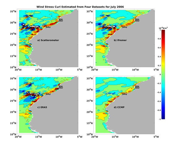
4.2. Wind Stress Issues

In addition to the previous comparisons mostly focusing on wind speed, the quality of wind direction is investigated from wind stress curl that is crucial for the correct representation of the Ekman pumping. If not provided by a particular analysis, wind stress is calculated using the COARE3.0 [17], with atmospheric boundary layer parameters taken from the ERA5.

Figure 8 and Figure 9 show monthly mean wind stress curl patterns estimated from the QuickSCAT scatterometer and wind analyses for the summer of 2006. Corresponding patterns for the ASCAT period (2016) are illustrated in the Appendix A (Figure A8 and Figure A9). The strongest wind stress curl features are present along continental coasts and around the Canary and Madeira Islands (Figure 8). The latter features are associated with island shadowing effects and wind acceleration in inter-island gaps (known as the Venturi effect) that produce downstream bands of accelerated and decelerated winds behind islands. These island shadowing and acceleration wind effects are properly resolved by all analyses but the CCMP (Figure 8). The positive wind vorticity pattern along the African coast is captured by all analyses with a somewhat weaker magnitude in the CCMP. Wind stress curl along the African coast is not homogeneous and is spatially modulated by orographic interactions over major capes along the Morocco–Mauritania coast (e.g., Cape Ghir, Sim, Juby [34]). All the above coastal features amplify in summer when the northeasterly trade winds strengthen.

Southern Hemisphere trade winds affecting the Benguela upwelling region also intensify in local summer (see January 2006 in Figure 9). As in the Canary region (Figure 8), the highest wind stress curl in the Benguela region is present along coastlines downstream of main capes (Cape Columbine and Cape of Good Hope). More details on wind stress curl patterns in the Canary and Benguela can be found in Desbiolles et al. (2014). Although the four wind sources exhibit qualitatively similar wind stress curl patterns in the Benguela region, all the analyses tend to smooth and underestimate the wind stress curl magnitude in comparison with purely scatterometer-based winds, with a stronger discrepancy in the CCMP. The CCMP has the weakest wind vorticity magnitude among the products. This suggests that Benguela upwelling simulations would be biased if forced by CCMP wind stress.

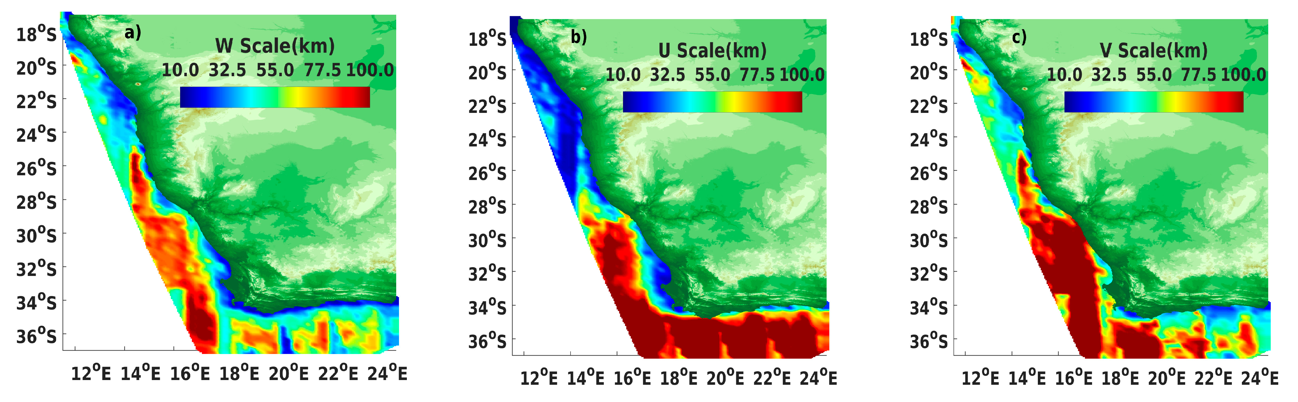
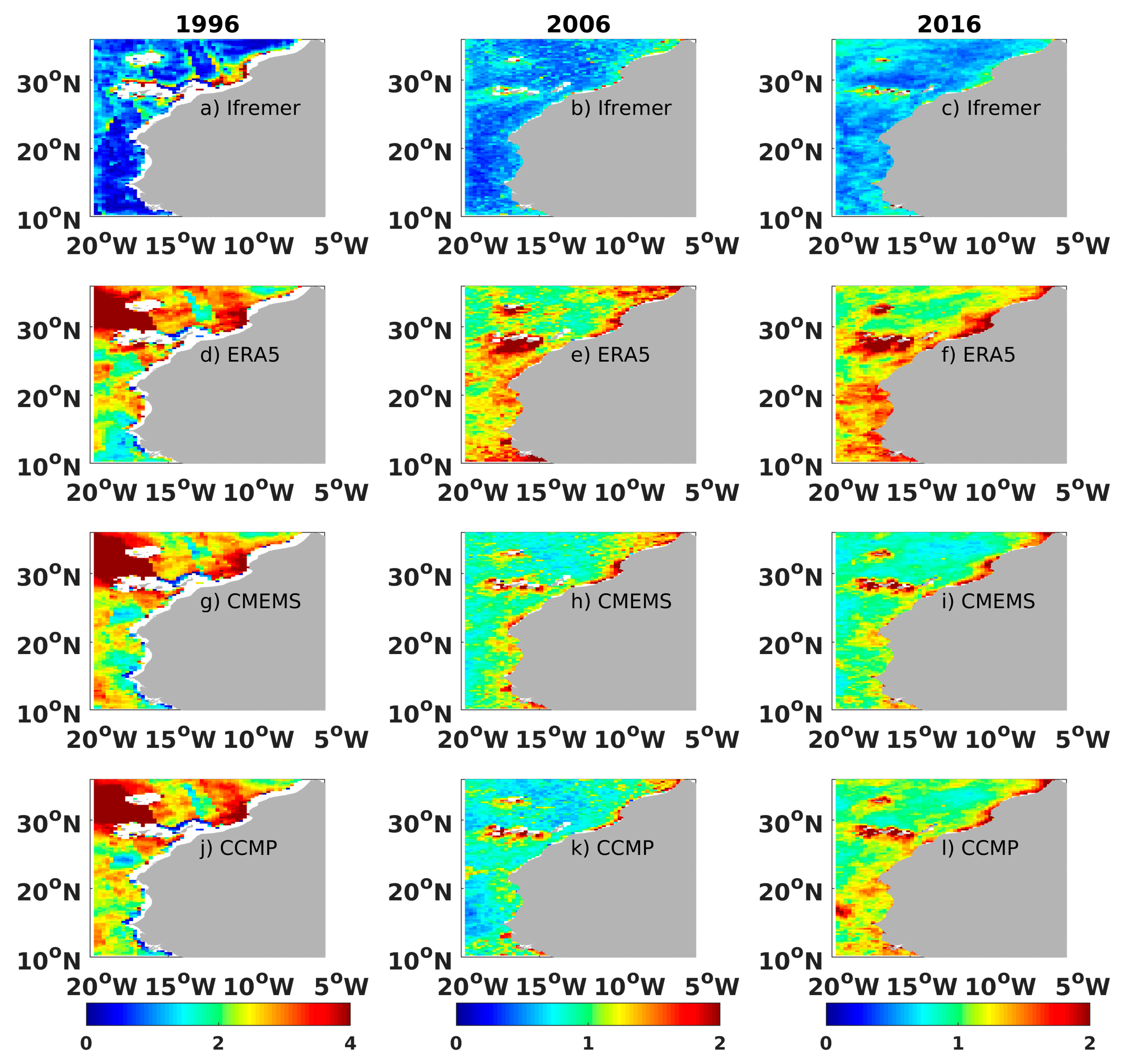
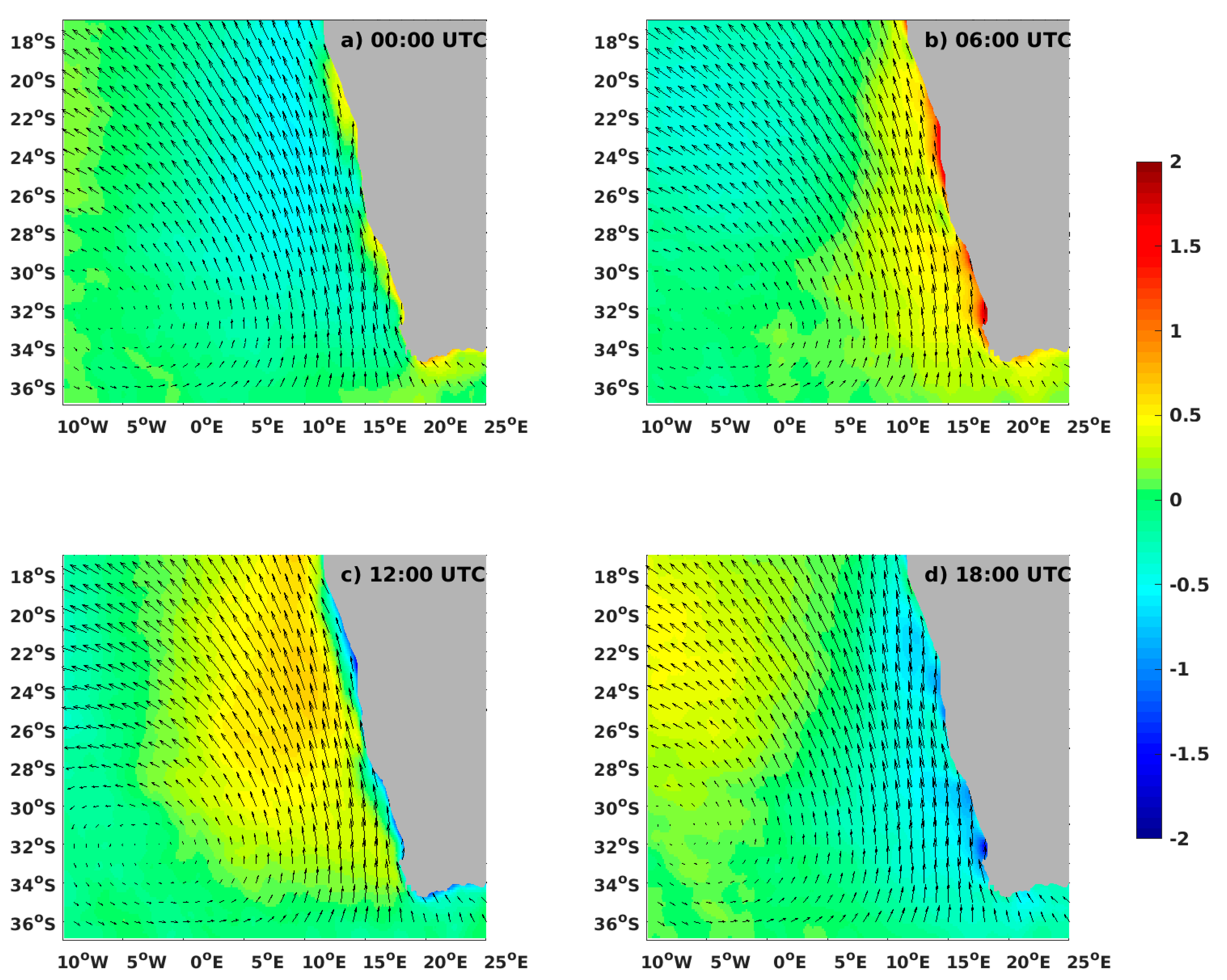
4.3. Assessment of the Local Wind Patterns

IFREMER satellite wind analysis captures significant diurnal variability of winds (Figure 10 and Figure 11) present in both the Canary and Benguela upwelling regions.

In the Canary region, the main diurnal pattern associated with wind acceleration at 6:00 UTC and deceleration at 18:00 UTC develops along the Moroccan coast. It resembles nocturnal jets developing due to diurnal changes in atmospheric boundary layer stability and height. The strongest variability in the low wind jet velocity occurs by the end of nocturnal cooling (6:00 UTC, sunrise) and day-time heating (18:00 UTC, sunset). Its diurnal magnitude is modulated by the coastal orography and amplifies to about 2 m s⁻¹ in the vicinity of Cape Ghir and Cape Blanc (21°N). Similar diurnal variability is present in the Benguela atmospheric low jet (Figure 11). In contrast to the Canary region (Figure 10), the diurnal wind variability extends beyond the coastal boundary in the Benguela region, which is an observation for which we do not have any immediate explanation. As in the Canary region, the diurnal magnitude of Benguela winds is spatially modulated along the coastline, reaching a local maximum of $1.5$ m s⁻¹ in St. Helena Bay (32°S, South Africa). This regional amplification is probably linked to summer season radiative heating and its impact on changes of Ta, SST, land temperature, and land–sea interactions.

5. Summary

This study presents the description and quality assessment of a regional coastal wind analysis with enhanced spatial and temporal resolution. This analysis referred to as IFREMER satellite wind analysis is currently available only over two major eastern boundary upwelling systems, the Canary and Benguela. For accuracy estimation purposes, the IFREMER analysis is also calculated over the California upwelling system, where several ground-truth mooring time series used are available. To the best of our knowledge, the IFREMER analysis provides a uniquely long time series of regional surface winds estimated from well-calibrated and homogenized scatterometer and radiometer data. It provides 27 years (1992 to 2018) of 10 m wind speed, zonal, and meridional velocity components, wind stress vector, along with its curl and divergence. Analysis uncertainty data are also provided at each grid cell. Data are available at synoptic times (00 h:00, 06 h:00, 12 h:00, and 18 h:00 UTC) on a regular 0.125° × 0.125° grid.

Even though the approach used for the determination of IFREMER 6-h winds is pretty similar to that used in the Copernicus/CMEMS (L4) wind reprocessing [16], some significant changes should be underlined. In this study, the determination of spatial structure functions is based on high spatial resolution winds from Sentinel-1A/B SAR, which allow for better characterization of fine spatial scale variability at each grid cell, including near coast cells. Temporal structure functions are also improved based on the use of consistent wind observations from all available scatterometers and radiometers (Table 1).

The accuracy of the methodology as resulting 6-h wind analysis is assessed from comparisons with ground-truth 6h-averaged NDBC buoy wind measurements. IFREMER wind analysis exhibits high accuracy in representing the wind speed and the related components temporal variability, with high correlation coefficients and quite low biases and RMSD values.

At regional scales, the new IFREMER satellite wind analysis and the three wind analyses (CMEMS, CMMP, and ERA5) are compared with purely scatterometer winds in the Canary and Benguela upwelling regions. Since the four analyses use mostly the same scatterometer retrievals, their comparison indicates the ability of each particular surface wind analysis methodology to resolve the spatial and temporal variability present in scatterometer observations. The four analyses exhibit comparable deviations from pure scatterometer winds for wind speed and components, wind stress and components, and wind stress curl. The IFREMER wind analysis has the lowest RMSD from the scatterometry in offshore and nearshore areas. Furthermore, excluding comparisons based on the use of poor scatterometer samplings (e.g., ERS-2), the IFREMER wind analysis does not show any time dependence in its deviation from the pure scatterometry.

We believe that these unique data have the potential to resolve various spatial and temporal wind characteristics at local scales (e.g., in cape areas) of both Canary and Benguela regions, including diurnal, seasonal, and annual variability. Further investigations of the IFREMER wind analysis content will be performed through the forcing ocean circulation model process. The latter is expected to better address the role of the high spatial and temporal surface wind variability on the coastal circulation. In the future, the surface wind analyses should address the fast, highly variable, and high wind conditions. The latter tend to be smoother in all surface wind analyses. Further improvements, as required by oceanic and atmospheric modelers, include the enhancement of the temporal resolution of the scatterometer wind analyses. The latter would be achieved through the use of a new approach including numerical modeling and data learning methods. Additional scatterometer missions such as ASCAT-C, HY-2b, HY-2c, and CFOSAT will be considered in a reprocessed long time series of IFREMER wind analyses.

The long time series datasets will be available from IFREMER data center CERSAT (http://cersat.ifremer.fr/ (accessed on 2 March 2021)). In the meantime, the data can be downloaded from (ftp://ftp.ifremer.fr/ifremer/cersat/projects/upwesatwind (accessed on 2 March 2021)). For the Canary or Benguela regions, each 6-h analysis file contains wind speed and velocity components, wind stress and its components, wind stress divergence and curl on a 0.125° × 0.125° grid. Supplementary information such as error estimate is also provided. Data are in NetCDF 4 format.

References

1. Desbiolles, F.; Blanke, B.; Bentamy, A.; Grima, N. Origin of fine-scale wind stress curl structures in the Benguela and Canary upwelling systems. J. Geophys. Res. Oceans 2014, 119, 7931–7948. [Google Scholar] [CrossRef] [Green Version]
2. Desbiolles, F.; Blanke, B.; Bentamy, A. Short-term upwelling events at the western African coast related to synoptic atmospheric structures as derived from satellite observations. J. Geophys. Res. Oceans 2014, 119, 461–483. [Google Scholar] [CrossRef] [Green Version]
3. Wang, D.; Gouhier, T.C.; Menge, B.A.; Ganguly, A.R. Intensification and spatial homogenization of coastal upwelling under climate change. Nat. Cell Biol. 2015, 518, 390–394. [Google Scholar] [CrossRef] [PubMed]
4. Pérez-Santos, I.; Seguel, R.; Schneider, W.; Linford, P.; Donoso, D.; Navarro, E.; Amaya-Cárcamo, C.; Pinilla, E.; Daneri, G. Synoptic-scale variability of surface winds and ocean response to atmospheric forcing in the eastern austral Pacific Ocean. Ocean Sci. 2019, 15, 1247–1266. [Google Scholar] [CrossRef] [Green Version]
5. Skamarock, W.C.; Klemp, J.B. A time-split nonhydrostatic atmospheric model for weather research and forecasting applications. J. Comput. Phys. 2008, 227, 3465–3485. [Google Scholar] [CrossRef]
6. García-Reyes, M.; Largier, J. Observations of increased wind-driven coastal upwelling off central California. J. Geophys. Res. Space Phys. 2010, 115, C04011. [Google Scholar] [CrossRef] [Green Version]
7. Freeman, E.; Woodruff, S.D.; Worley, S.J.; Lubker, S.J.; Kent, E.C.; Angel, W.E.; Berry, D.I.; Brohan, P.; Eastman, R.; Gates, L.; et al. ICOADS Release 3.0: A major update to the historical marine climate record. Int. J. Clim. 2017, 37, 2211–2232. [Google Scholar] [CrossRef] [Green Version]
8. Bentamy, A.; Grodsky, S.A.; Elyouncha, A.; Chapron, B.; Desbiolles, F. Homogenization of scatterometer wind retrievals. Int. J. Clim. 2017, 37, 870–889. [Google Scholar] [CrossRef] [Green Version]
9. Blanke, B.; Speich, S.; Bentamy, A.; Roy, C.; Sow, B. Modeling the structure and variability of the southern Benguela upwelling using QuikSCAT wind forcing. J. Geophys. Res. Space Phys. 2005, 110, C07018. [Google Scholar] [CrossRef] [Green Version]
10. Capet, X.; Colas, F.; McWilliams, J.; Penven, P.; Marchesiello., P. Eddies in eastern boundary subtropical upwelling systems. In Ocean. Modeling in an Eddying Regime; Hecht, M.W., Hasumi, H., Eds.; Wiley: Hoboken, NJ, USA, 2008; Volume 177, pp. 131–147. [Google Scholar] [CrossRef] [Green Version]
11. Renault, L.; Dewitte, B.; Marchesiello, P.; Illig, S.; Echevin, V.; Cambon, G.; Ramos, M.; Astudillo, O.; Minnis, P.; Ayers, J.K. Upwelling response to atmospheric coastal jets off central Chile: A modeling study of the October 2000 event. J. Geophys. Res. Space Phys. 2012, 117, C02030. [Google Scholar] [CrossRef] [Green Version]
12. Grodsky, S.A.; Kudryavtsev, V.N.; Bentamy, A.; Carton, J.A.; Chapron, B. Does direct impact of sst on short wind waves matter for scatterometry ? Geophys. Res. Lett. 2012, 39, L12602. [Google Scholar] [CrossRef] [Green Version]
13. Muñoz, E.; Weijer, W.; Grodsky, S.A.; Bates, S.C.; Wainer, I. Mean and Variability of the Tropical Atlantic Ocean in the CCSM4. J. Clim. 2012, 25, 4860–4882. [Google Scholar] [CrossRef] [Green Version]
14. Chelton, D.B.; Schlax, M.G.; Freilich, M.H.; Milliff, R.F. Satellite Measurements Reveal Persistent Small-Scale Features in Ocean Winds. Science 2004, 303, 978–983. [Google Scholar] [CrossRef] [PubMed] [Green Version]
15. O’Neill, L.W.; Chelton, D.B.; Esbensen, S.K. The effects of sst-induced surface wind speed and direction gradients on midlatitude surface vorticity and divergence. J. Clim. 2010, 23, 255–281. [Google Scholar]
16. Desbiolles, F.; Bentamy, A.; Blanke, B.; Roy, C.; Mestas-Nuñez, A.M.; Grodsky, S.A.; Herbette, S.; Cambon, G.; Maes, C. Two decades [1992–2012] of surface wind analyses based on satellite scatterometer observations. J. Mar. Syst. 2017, 168, 38–56. [Google Scholar] [CrossRef] [Green Version]
17. Fairall, C.W.; Bradley, E.F.; Hare, J.E.; Grachev, A.A.; Edson, J.B. Bulk Parameterization of Air-Sea Fluxes: Updates and Verification for the COARE3.0 Algorithm. J. Clim. 2003, 16, 571–591. [Google Scholar] [CrossRef]
18. Bentamy, A.; Queffeulou, P.; Quilfen, Y.; Katsaros, K. Ocean surface wind fields estimated from satellite active and passive microwave instruments. IEEE Trans. Geosci. Remote Sens. 1999, 37, 2469–2486. [Google Scholar] [CrossRef]
19. Wentz, F.J.; Smith, D.K. A model function for the ocean-normalized radar cross section at 14 GHz derived from NSCAT observations. J. Geophys. Res. Space Phys. 1999, 104, 11499–11514. [Google Scholar] [CrossRef]
20. Hersbach, H.; Stoffelen, A.; De Haan, S. An improved C-band scatterometer ocean geophysical model function: CMOD5. J. Geophys. Res. Space Phys. 2007, 112, C03006. [Google Scholar] [CrossRef]
21. Bentamy, A.; Grodsky, S.A.; Chapron, B.; Carton, J.A. Compatibility of C-and Ku-band scatterometer winds: ERS-2 and QuikSCAT. J. Mar. Syst. 2013, 117–118, 72–80. [Google Scholar] [CrossRef] [Green Version]
22. Grodsky, S.A.; Carton, J.A.; Nigam, S.; Okumura, Y.M. Tropical Atlantic Biases in CCSM4. J. Clim. 2012, 25, 3684–3701. [Google Scholar] [CrossRef] [Green Version]
23. Tomita, H.; Kubota, M. An analysis of the accuracy of Japanese Ocean Flux data sets with Use of Remote sensing Observations (J-OFURO) satellite-derived latent heat flux using moored buoy data. J. Geophys. Res. Space Phys. 2006, 111, C07007. [Google Scholar] [CrossRef] [Green Version]
24. Atlas, R.; Hoffman, R.N.; Ardizzone, J.; Leidner, S.M.; Jusem, J.C.; Smith, D.K.; Gombos, D. A Cross-calibrated, Multiplatform Ocean Surface Wind Velocity Product for Meteorological and Oceanographic Applications. Bull. Am. Meteorol. Soc. 2011, 92, 157–174. [Google Scholar] [CrossRef]
25. Ebuchi, N.; Graber, H.C.; Caruso, M.J. Evaluation of Wind Vectors Observed by QuikSCAT/SeaWinds Using Ocean Buoy Data. J. Atmos. Ocean. Technol. 2002, 19, 2049–2069. [Google Scholar] [CrossRef]
26. Bentamy, A.; Croize-Fillon, D.; Perigaud, C. Characterization of ASCAT measurements based on buoy and QuikSCAT wind vector observations. Ocean Sci. 2008, 4, 265–274. [Google Scholar] [CrossRef] [Green Version]
27. Verspeek, J.; Stoffelen, A.; Portabella, M.; Bonekamp, H.; Anderson, C.; Saldana, J. Validation and Calibration of ASCAT Using CMOD5.n. IEEE Trans. Geosci. Remote Sens. 2009, 48, 386–395. [Google Scholar] [CrossRef]
28. Yamartino, R.J. A Comparison of Several "Single-Pass" Estimators of the Standard Deviation of Wind Direction. J. Clim. Appl. Meteorol. 1984, 23, 1362–1366. [Google Scholar] [CrossRef] [Green Version]
29. Freilich, M.H.; Dunbar, R.S. The accuracy of the NSCAT-1 vector winds: Comparison with NDBC buoys. J. Geophys. Res. 1999, 104, 246. [Google Scholar]
30. Dee, D.P.; Uppala, S.M.; Simmons, A.J.; Berrisford, P.; Poli, P.; Kobayashi, S.; Andrae, U.; Balmaseda, M.A.; Balsamo, G.; Bauer, D.P.; et al. The ERA-Interim reanalysis: Configuration and performance of the data assimilation system. Q. J. R. Meteorol. Soc. 2011, 137, 553–597. [Google Scholar] [CrossRef]
31. Hersbach, H.; de Rosnay, P.; Bell, B.; Schepers, D.; Simmons, A.; Soci, C.; Abdalla, S.; Alonso-Balmaseda, M.; Balsamo, G.; Bechtold, P.; et al. Operational global reanalysis: Progress, future directions and synergies with NWP. ERA Rep. Ser. 2018. [Google Scholar] [CrossRef]
32. Rivas, M.B.; Stoffelen, A. Characterizing ERA-Interim and ERA5 surface wind biases using ASCAT. Ocean Sci. 2019, 15, 831–852. [Google Scholar] [CrossRef] [Green Version]
33. Bentamy, A.; Fillon, D.C. Gridded surface wind fields from Metop/ASCAT measurements. Int. J. Remote Sens. 2011, 33, 1729–1754. [Google Scholar] [CrossRef] [Green Version]
34. Sangrà, P.; Troupin, C.; Barreiro-González, B.; Barton, E.D.; Orbi, A.; Arístegui, J. The C ape G hir filament system in A ugust 2009 (NW Africa). J. Geophys. Res. Oceans 2015, 120, 4516–4533. [Google Scholar] [CrossRef] [Green Version]
Figure 1. National Data Buoy Center (NDBC) buoy locations. Red and blue symbols show coastal (<50 km of coastlines) and offshore buoys, respectively. (a) Panel shows all buoy locations, while (b) shows only buoys located in the Californian basin.
Remotesensing 13 00940 g001
Figure 2. Spatial scales (km) of 10m wind speed (a,d,g), zonal wind (b,e,h), and meridional wind (c,f,i) structure functions estimated from Sentinel-1a and Sentinel-1b synthetic aperture radar (SAR) IW retrievals during 2017–2019 over Benguela (top), Canary (middle), and California (bottom) upwelling zones.
Remotesensing 13 00940 g002aRemotesensing 13 00940 g002b
Figure 3. Spatial distribution of lagged temporal correlations of 10 m wind speed (a,d,g), zonal wind (b,e,h), and meridional wind (c,f,i) estimated from homogenized remotely sensed winds [8] in January and July 2000 over Benguela (top), Canary (middle), and California (bottom) upwelling zones. Time lag is included in each panel.
Remotesensing 13 00940 g003
Figure 4. Offshore comparisons of 6-hourly averaged buoy and on one hand IFREMER satellite analyses (left column), and on other hand ERA5 re-analyses (right column). Panels (a,b) illustrate wind speed comparisons, (c,d) illustrate zonal wind component comparisons, and (e,f) illustrate meridional wind component comparisons. Colors indicate sampling length values. Black and green lines indicate the perfect and symmetrical regression lines, respectively.
Remotesensing 13 00940 g004
Figure 5. As Figure 4 but for nearshore comparisons.
Remotesensing 13 00940 g005
Figure 6. Spatial distribution of root mean square difference (RMSD) between 10 m neutral wind speed from collocated scatterometer retrievals and (ac) IFREMER satellite wind analysis, (df) ERA5 reanalysis, (gi) CMEMS satellite wind analysis, and (jl) CCMP analysis over the Canary upwelling zone. Note that retrievals from different scatterometers are used in 1996 (ERS2, left column), 2006 (QuikSCAT, middle column), and 2016 (ASCAT, right column). Colors indicate RMSD in m s−1. Note that color scale limits for 1996 are different from those in 2006 and 2016.
Remotesensing 13 00940 g006
Figure 7. The same as in Figure 6 but for the Benguela upwelling region.
Remotesensing 13 00940 g007
Figure 8. July 2006 mean of wind stress curl estimated from (a) scatterometer (QuikSCAT) and collocated (b) Ifremer, (c) ERA-5, and (d) CCMP analyses over the Canary zone. Colors indicate curl amplitude in N/m3.
Remotesensing 13 00940 g008
Figure 9. The same as in Figure 8 but over the Benguela zone in January 2006.
Remotesensing 13 00940 g009
Figure 10. Diurnal 10 m wind speed anomaly (shaded, m s−1) estimated as the difference between the seasonal mean for a given synoptic time and the seasonal mean for all synoptic times for January, and the seasonal mean wind velocity for each synoptic time. Results are based on the IFREMER wind analysis, seasonal means are computed over 2000–2018.
Remotesensing 13 00940 g010
Figure 11. The same as in Figure 10 but for the Benguela region in July.
Remotesensing 13 00940 g011