Abstract
In this paper, based on electrical power consumption (EPC) data extracted from DMSP/OLS night light data, we select three national-level urban agglomerations in China’s Yangtze River Economic Belt(YREB), includes Yangtze River Delta urban agglomerations(YRDUA), urban agglomeration in the middle reaches of the Yangtze River(UAMRYR), and Chengdu-Chongqing urban agglomeration(CCUA) as the research objects. In addition, the coefficient of variation (CV), kernel density analysis, cold hot spot analysis, trend analysis, standard deviation ellipse and Moran’s I Index were used to analyze the Spatio-temporal Dynamic Evolution Characteristics of EPC in the three urban agglomerations of the YREB. In addition, we also use geographically weighted regression (GWR) model and random forest algorithm to analyze the influencing factors of EPC in the three major urban agglomerations in YREB. The results of this study show that from 1992 to 2013, the CV of the EPC in the three urban agglomerations of YREB has been declining at the overall level. At the same time, the highest EPC value is in YRDUA, followed by UAMRYR and CCUA. In addition, with the increase of time, the high-value areas of EPC hot spots are basically distributed in YRDUA. The standard deviation ellipses of the EPC of the three urban agglomerations of YREB clearly show the characteristics of “east-west” spatial distribution. With the increase of time, the correlations and the agglomeration of the EPC in the three urban agglomerations of the YREB were both become more and more obvious. In terms of influencing factor analysis, by using GWR model, we found that the five influencing factors we selected basically have a positive impact on the EPC of the YREB. By using the Random forest algorithm, we found that the three main influencing factors of EPC in the three major urban agglomerations in the YREB are the proportion of secondary industry in GDP, Per capita disposable income of urban residents, and Urbanization rate.
1. Introduction
Energy is not only an important material resource for human survival and activities, but also a basic driving force for economic growth and social progress [1]. Electric energy is recognized as one of the most economical and efficient energy sources in the world and plays an important role in the development of the national economy [2]. As an important component of energy, electricity relates to every aspect of commercial activities, industrial productions, and urban residents’ daily activities [3]. Electricity is one of the most important components in energy consumption, which is directly related to economic growth, CO2 emission and global warming [4]. Changes in electrical power consumption (EPC) patterns of a country over a period of time reflect on its socio-economic development and energy utilization processes [5]. Electricity resources are an important part of china energy resources and play a very important role in the sustained economic development and the improvement of people’s lives [6]. China’s rapid economic development in the last 20 years has resulted in increased demand for electricity and ensuing shortages in electric power supply [7]. China’s growing EPC has become an important factor to improving socio-economic development, as well as aggravating environmental degradation [8]. EPC is one of the basic indices for evaluating electric power use [9]. Obtaining timely and accurate data on the spatiotemporal dynamics of EPC is crucial for the effective utilization of electric power in China [10].
As a popular topic in studies of urban sustainability and regional economics, EPC has been widely studied at large scales [11]. At present, EPC mainly uses administrative regions as the basic statistical unit. It is difficult to provide spatial distribution information within the administrative unit, and cannot fully reveal the spatial difference of EPC, which hinders the integration and comprehensive analysis of EPC data with other socioeconomic and natural factors [12]. Therefore, spatial research on EPC has become a current hot spot. Compared to traditional socioeconomic census, remote sensing techniques provide a suitable method for describing the spatial distribution of EPC [13]. The Operational Linescan System (OLS) sensor mounted on the Defense Meteorological Satellite Program (DMSP) of the US military weather satellite can effectively detect the low-intensity night lights generated by urban night lights and even small-scale residential areas and traffic flows. Therefore, it is widely regarded as a good data source for monitoring the intensity of human activities [14]. At present, academia has carried out a lot of research work using DMSP-OLS night light data. From the perspective of research content, it mainly includes urban expansion [15,16,17,18], economic estimation [19,20,21,22], energy consumption [23,24,25,26] and population estimation [27,28,29,30]. Therefore, since the 1980s, domestic and foreign scholars have used DMSP/OLS night light data to conduct a lot of research on EPC [31]. From the point of view of the research objects, it is mainly based on the global [32,33,34,35,36], China [37,38,39,40,41], and India [42,43,44]; from the perspective of the research content, it is mainly based on the estimation of EPC [45,46,47,48] and Spatialization [49,50,51,52]. By summarizing, we can clearly find that the current research on EPC based on DMSP/OLS night light data has relatively few studies on large-scale cross-regional urban agglomerations within a country.
China’s Yangtze River Economic Belt (YREB) is an important first-level development axis in the “T”-shaped spatial structure strategy of China’s land development and economic layout. It forms the golden corridor of China’s economic development with the coastal economic belt [53]. Specifically, YREB includes three national-level urban agglomerations: Yangtze River Delta urban agglomerations(YRDUA), urban agglomeration in the middle reaches of the Yangtze River(UAMRYR), and Chengdu-Chongqing urban agglomeration(CCUA). Based on YREB’s special importance status, the current academic circles have carried out a lot of research work on YREB, and many research results have been obtained. Specifically, in terms of research methods, it mainly includes gravity model [54,55,56], social network analysis [57,58,59], coupling coordination model [60,61,62] and spatial autocorrelation method [63,64,65]. In terms of research content, it mainly includes urban expansion [66,67,68,69], ecological environment [70,71,72,73], industrial development [74,75,76,77], economic growth [78,79,80,81]. By summarizing, it is obvious that there is less research on the EPC of YREB.
Therefore, according to the current research status, this paper is based on the EPC data extracted from DMSP/OLS night light data, and chooses the three urban agglomerations (YRDUA, UAMRYR and CCUA) of YREB in China as the research objects. Next, we using coefficient of variation, kernel density analysis, hot spot analysis, trend analysis, standard deviation ellipse, spatial autocorrelation analysis to analyze the Spatio-temporal Dynamic Evolution Characteristics of the EPC of the three urban agglomerations of YREB in China. In addition, we also use Geographic weighted regression (GWR) model and random forest algorithm to analyze the influencing factors of the EPC of the three major urban agglomerations in YREB. This paper is a comparative analysis of the Spatio-temporal Dynamic Evolution Characteristics of the EPC of the three urban agglomerations of YREB in China. The purpose is to more clearly discover the Spatio-temporal Dynamic Evolution Characteristics of the EPC of the three urban agglomerations of YREB in China. Moreover, we can also calculate and analyze the influencing factors of the EPC of the three major urban agglomerations in YREB. The research work of this paper can enrich the depth and breadth of EPC-related research based on DMSP/OLS night light data at the theoretical level, and has certain theoretical significance. In addition, the research work in this paper can also provide scientific basis for the optimization of electricity resources allocation and scientific formulation of electricity control plans for the three urban agglomerations of YREB in China at the practical level, so it also has certain practical significance.
2. Research Area and Data Sources
2.1. Research Area
YREB spans the three major regions of China’s east, middle and west, covering 11 provinces and cities including Shanghai, Jiangsu, Zhejiang, Anhui, Jiangxi, Hubei, Hunan, Chongqing, Sichuan, Yunnan, and Guizhou, covering an area of approximately 2.0523 million square kilometers, accounting for 21.35% of China’s total area. The location introduction map of the YREB and its three major urban agglomerations is shown in Figure 1. As of the end of 2018, YREB’s total population and GDP were 599 million people and 40.30 trillion-yuan, accounting for 42.91% and 44.76% of China’s total, respectively.
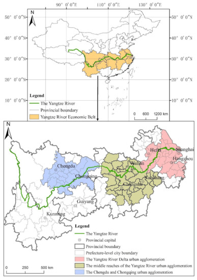
Figure 1.
Location introduction map of YREB and its three major urban agglomerations.
YREB includes three national-level urban agglomerations, YRDUA, UAMRYR and CCUA. These three urban agglomerations are the main part of YREB. The zoning area, permanent population, and total economic volume of YREB’s three national-level urban agglomerations accounted for 34.78%, 63.61% and 79.41% of the total YREB respectively. The specific statistical information of these three major urban agglomerations is shown in Figure 2. In September 2016, the “YREB Development Plan Outline” was officially issued, one of the main contents is to establish YREB’s three-pole development status with the three national urban agglomerations of YRDUA, UAMRYR and CCUA. Therefore, it is necessary to give full play to the radiation role of these three urban agglomerations to create three growth poles of YREB. However, the three major urban agglomerations still have obvious gaps in many aspects such as GDP, city size and population. Therefore, it is essential to compare and analyze the three major urban agglomerations of YREB. In addition, the work flow chart of this paper is shown in Figure 3.
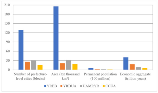
Figure 2.
Statistics of the specific scale of YREB and its three major urban agglomerations (as of the end of 2018).
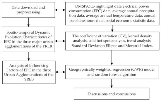
Figure 3.
The workflow of this paper.
2.2. Data Sources
The DMSP/OLS night light images used in this paper are download from the National Geophysical Data Center (NGDC) (https://ngdc.noaa.gov/eog/dmsp/downloadV4composites.html), with a data span of 1992–2013, and the light gray value range is 0–63. The DMSP/OLS night light data have a spatial resolution of 30 arc seconds (Arc Second) (about 1 km at the equator) [82]. It providing a global annual raster image that calibrates the average light intensity at night, including the persistent light sources in cities, villages, and other locations, and removing the effects of interference noise, such as moonlight, clouds, fire, oil, and gas combustion [83]. The EPC data [84] used in this paper were mainly obtained from a model simulation based on corrected night light data, with a spatial resolution of 1 km, a time resolution of years, and a unit of 104 kWh. The processing of EPC data includes: (1) Based on the DMSP-OLS radiation correction data in 2006, time sequence correction and oversaturation correction were performed on the DMSP-OLS stable night light data from 1992 to 2013. (2) According to the similarity of urban development level and spatial distribution, the world is divided into 48 sub-regions, and the EPC statistics data in each sub-region are used to train power consumption estimation models. (3) This estimation model was applied to the corrected DMSP-OLS pixel by pixel to produce 1000 m global EPC data product data. The EPC data is downloaded from the Yangtze River Delta Science Data Center, National Earth System Science Data Sharing Infrastructure, National Science & Technology Infrastructure of China (http://nnu.geodata.cn:8008/). The EPC statistics for the YREB in 2013 are shown in Figure 4.
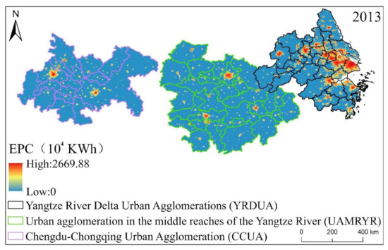
Figure 4.
The estimated EPC in the three major urban agglomerations of YREB in 2013 based on intercalibrated NSL data.
Influencing factor data such as GDP per capita, urbanization rate, per capita disposable income of urban residents, the total retail sales of social consumer goods, total social investment in fixed assets, urban built-up area, the proportion of primary industry in GDP, the proportion of secondary industry in GDP, the proportion of tertiary industry in GDP are all downloaded from YREB Big Data Platform (http://yreb.sozdata.com, accessed on 15 December 2020) and China Economic and Social Big Data Research Platform (https://data.cnki.net accessed on 20 December 2020). Other influencing factors average annual precipitation, average annual temperature, annual sunshine hours are all downloaded from the Resource Environmental Science and Data Center of the Chinese Academy of Sciences (http://www.resdc.cn/ accessed on 20 December 2020). The boundaries of administrative units at all levels are taken from the 1:4 million database of the National Basic Geographic Information Center.
3. Research Methods
3.1. Coefficient of Variation
In probability theory and statistics, the coefficient of variation (CV), also known as the “dispersion coefficient”, is one of the most commonly used statistics to measure the degree of dispersion of each observation. This coefficient is expressed as the coefficient of variation (CV) and defined as the ratio of the standard deviation to the average. Geography circles widely use the coefficient of variation (CV) method to study spatial differences. Its advantage is that it can eliminate the influence of different units and averages on the results [85]. Therefore, this paper uses the coefficient of variation (CV) method to measure and reveal the relative differences of EPC among the three major urban agglomerations in the YREB. The calculation formula is as follows:
In the formula, CVCV is the coefficient of variation. The larger the value of CVCV is, the greater the relative difference in regional power consumption will be. is the standard deviation of observations, and is the average value of the observations.
3.2. Kernel Density Estimation
Kernel density estimation method [86] is a nonparametric estimation method which can get smooth estimation of density function. It is mainly used to estimate the probability density of random variables [87]. Therefore, kernel density estimation has strong adaptability and can obtain more general and broad conclusions. The kernel density equation of EPC with point P as the center is as follows [88]:
In the formula, n represents the number of administrative units included in the distance scale; k represents the kernel density function; h represents the distance threshold, which is the scale of the kernel density estimation method; d(x, xi) represents the Euclidean distance between two points.
3.3. Hot Spot Analysis
Hot spot analysis can detect the non-randomness of the spatial distribution of events and calculate the hot spot areas where the frequency of events occurs is high [89]. Hot spots and cold spots refer to areas where the distribution of the characteristic values of services are high or low. Hot spots require elements to have high values and be surrounded by other elements that also have high values [90]. On this basis, this paper uses the hot spot analysis (Getis-Ord Gi*) tool to analyze the spatial pattern distribution characteristics of the hot and cold spots of the EPC of the three major urban agglomerations in YREB. The calculation formula is as follows [91]:
In the formula, is the mathematical expectation value; is the coefficient of variation. When is positively significant, it means that the value around the spatial unit i is relatively large, that is, it becomes a hot spot; when is negatively significant, it means that the spatial unit i is a low-value spatial cluster, that is, become a cold spot.
3.4. Trend Analysis
The trend analysis is based on the temporal change trends of a single pixel to reflect the overall law of spatial changes to comprehensively reflect the evolution of regional spatial and temporal patterns. For an administrative unit with a significant change in EPC, the trend type is determined by calculating the slope of the change in EPC from 1992 to 2013. Therefore, we used ArcGIS and ENVI software to analyze the EPC trend of YREB’s three urban agglomerations from 1992 to 2013 and conducted a comparative analysis. The calculation formula is as follows [92].
In the formula, n is the number of years from 1992 to 2013, that is, n = 22; xi is the serial number from 1992 to 2013, and Ei represents the EPC of a certain administrative unit in year i. Slope < 0 indicates that the EPC of the administrative unit is showing a significant decreasing trend, slope > 0 indicates that the EPC is increasing significantly. For the administrative units with increasing EPC, according to their slope mean and standard deviation, they are divided into five types: rapid growth, faster growth, moderate growth, slow growth and slower growth.
3.5. Standard Deviation Ellipse
Standard deviational ellipse (SDE) is a spatial statistical method that reveals the multi-faceted features of a variable spatial distribution [93]. The SDE reflects the center of gravity, the degree of dispersion of the secondary trend, and the main trend direction of an element based on its two-dimensional spatial distribution through the center, along the main axis, along the auxiliary axis, at the azimuth angle, etc. [94]. The formula is as follows.
The center of gravity is calculated as:
The SDE is calculated as:
3.6. Moran’s I Index
Spatial autocorrelation is a spatial statistical analysis method that can be used to measure the correlation of a certain geographical phenomenon at a location or the value of an attribute with the same phenomenon or attribute value at a nearby location [67]. Moran’s I is a powerful tool for identifying spatial clustering effects. Global Moran’s I and local Moran’s I are calculated to associate anomaly correlations at neighboring grid cells with one another [95]. At present, the global Moran’s I index, proposed by Moran [96], is extensively used to test the spatial dependence of a specific statistical indicator between the adjacent regions in the entire space-time system [97].
Local spatial autocorrelation analysis can reveal the heterogeneous characteristics of local spatial differences, and further fully reflect the regional EPC spatial associations and difference trends. At present, the main indicators for measuring local spatial autocorrelation are Moran scatter plots and spatially linked local indicators (LISA) [98]. The Moran scatter plot is a measurement index reflecting local spatial stability and can visually illustrate the form of the spatial connections between research units. LISA can measure the significance of this spatial connection and the difference between the attributes of the regional unit and its surrounding areas [99]. Therefore, this study combines the global Moran’s I index, local Moran scatter plot, and LISA to monitor the spatial agglomeration and local spatial instability of EPC in the YREB at different scales. The calculation formula is as follows [88].
(1) Global autocorrelation analysis.
(2) Local autocorrelation analysis.
In the formula, xi, xj represents the EPC of the two administrative units i and j; n is the total number of samples, representing all the administrative units being analysed ; Wij is the spatial weight matrix, which is defined in this paper by the adjacency criterion. When administrative unit i is adjacent to administrative unit j, Wij = 1, otherwise, Wij = 0, i = 1,2, …,n, j = 1,2, …,m.
3.7. Geographically Weighted Regression (GWR) Model
GWR methods is a technique for exploring statistical associations between a dependent variable and a set of explanatory variables [100]. GWR is a localized regression model which allows the estimated parameters to vary over the spatial domain. It also takes spatial autocorrelation into account and thus can mitigate the bias in models caused by the spatial autocorrelation effect. Hence, compared with the global regression model in which parameter estimation is fixed for each observation, GWR can be used to address the spatial nonstationarity and spatial autocorrelation of observations and determine whether the underlying process exhibits spatial heterogeneity. The formula is as follows:
In the formula, is the center coordinate of position i, is the regression coefficient of the k-th variable at position i, , are the intercept and error terms of the model at position i, respectively.
3.8. Random Forest Algorithm
The random forest algorithm has been widely used to solve numerous kinds of regression and classification tasks [101]. This is because random forest is a user-friendly machine learning method that can almost always produce desirable results without tedious parameter tuning [102]. In the training stage, the random forest algorithm uses bootstrap sampling to collect multiple sub-training datasets from the input training dataset to train multiple decision trees successively. Notably, the random forest algorithm evaluates the importance of variables through variable importance measures, which represents the total decrease in node impurity from splitting on the variable as measured for regression by the residual sum of squares and averaged over all trees [103]. In this research, we use the random forest algorithm to analyze the influence of the factors affecting the EPC of the three major urban agglomerations in the YREB. Influencing factors include GDP per capita, urbanization rate, per capita disposable income of urban residents, the total retail sales of social consumer goods, total social investment in fixed assets, urban built-up area, the proportion of primary industry in GDP, the proportion of secondary industry in GDP, the proportion of tertiary industry in GDP, average annual precipitation, average annual temperature, and annual sunshine hours. The random forest algorithm implemented in Python 3.7 software.
4. Results
4.1. Temporal and Spatial Evolution Characteristics of EPC of YREB Three Urban Agglomerations at Different Scales
From Figure 5, we can see that from 1992 to 2013, the CV of the three major urban agglomerations of YREB has been in a downward trend at the overall level. The value dropped from 8.08 in 1992 to 2.98 in 2013, with an average annual decrease of −2.87%, reflecting that the overall EPC difference of YREB’s three major urban agglomerations is gradually decreasing. Specifically, the CV of the three major urban agglomerations of YREB is also in a downward trend. Among them, the CV of YRDUA dropped from 5.12 in 1992 to 1.75 in 2013, with an average annual decrease of −2.99%. UAMRYR’s CV dropped from 9.88 in 1992 to 4.17 in 2013, with an average annual decrease of −2.63%. CCUA’s CV dropped from 12.08 in 1992 to 4.18 in 2013, with an average annual decrease of −2.97%. We can find that the CV declines of these three urban agglomerations are very close, reflecting that the EPC differences within these three urban agglomerations have been shrinking from 1992 to 2013.
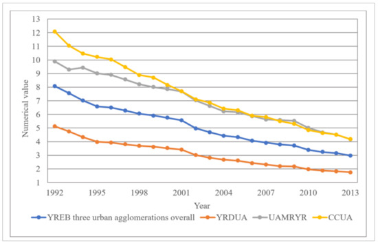
Figure 5.
The statistical graph of the CV trend of the EPC of YREB’s three major urban agglomerations from 1992 to 2013.
In addition, through comparison, we can find that in terms of the comparison of the size of CV, the value of CCUA is the largest, the value of UAMRYR is second, and the value of YRDUA is the smallest. This is because CCUA is located in the western region of China. The overall economic development of CCUA is lagging behind YRDUA and UAMRYR. In CCUA, all provinces and cities are doing their best to develop their own provincial capital cities and a few prefecture-level cities, which directly results in the comprehensive development gap between provincial capital cities and a few prefecture-level cities and other regions is getting wider and wider. Since the development of various undertakings such as economic development and urbanization construction will consume a large amount of power resources, this directly leads to the increasing EPC gap between provincial capitals and a few cities and other regions. Therefore, the CV of CCUA is the largest among the three major urban agglomerations in the YREB. The overall development of UAMRYR is slightly better than that of CCUA. Therefore, the CV of UAMRYR’s EPC is slightly smaller than that of CCUA. YRDUA is located in the eastern area of China, and it is also one of the most developed regions in China. Most of the areas within its area are relatively developed. On the overall level, the development of internal administrative units at all levels is significantly better than that of UAMRYR and CCUA, and the internal EPC gap is not very obvious. Therefore, the CV of YRDUA’s EPC is significantly smaller than UAMRYR and CCUA.
4.2. The Spatial Structure Evolution Characteristics of the EPC of the Three Major Urban Agglomerations of the YREB
From Figure 6, we can find that from 1992 to 2013, the EPC of the three major urban agglomerations of YREB was on an increasing trend. Specifically, through comparison, we can find that no matter what time period, the EPC of the three major urban agglomerations of YREB Continuous decreases from the east (YRDUA) to the central (UAMRYR) and the west (CCUA). And with the increase of time, the gap between the EPC of YRDUA and the EPC of UAMRYR and CCUA is also increasing, which directly reflects the obvious comprehensive development gap between the three urban agglomerations.
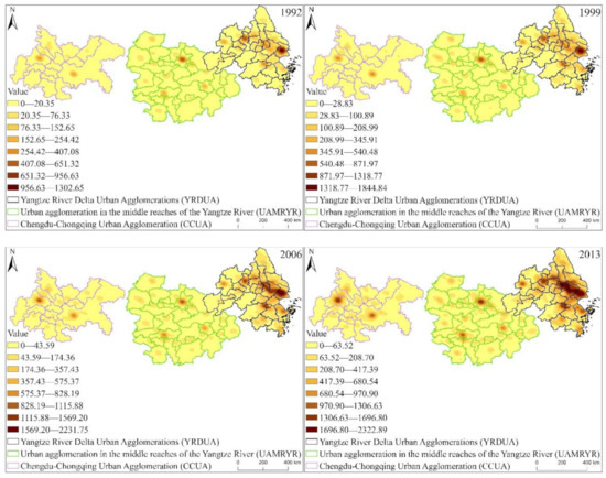
Figure 6.
EPC kernel density distribution of the three major urban agglomerations of YREB from 1992 to 2013.
Specifically, we can clearly find that in YRDUA, there are more cities with high EPC, and these cities are more developed. In UAMRYR and CCUA, areas with high EPC are provincial capitals and other major cities. Therefore, we conclude that the distribution of EPC levels is directly related to the distribution of cities. This characteristic is particularly obvious in the central and western regions, and with the increase of time, it will become more and more obvious. This is because the level of EPC is closely related to the city size, economic development level, and population size of this area.
4.3. The Evolution Characteristics of the Spatial Pattern of EPC in the Three Major Urban Agglomerations of the YREB
Based on the hot spot analysis tool, we can know where the high-value or low-value elements are clustered in space through the obtained z-score and p-value. The higher the z-score, the tighter the clusters of high values (hot spots), and conversely, the tighter the clusters of low values (cold spots).
From Figure 7, we can find that during 1992–2013, with the increase of time, the accumulation of cold and hot spots of YREB EPC became more and more obvious. At the same time, the distribution of high-value areas of EPC hotspots also obviously shows a characteristic of decreasing from YRDUA in the east to UAMRYR in the middle and CCUA in the west.
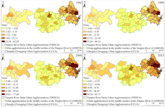
Figure 7.
The distribution statistics of EPC cold and hot spots in the three major urban agglomerations of YREB from 1992 to 2013.
Specifically, the high-value areas of EPC hot spots are concentrated in YRDUA, and this distribution becomes more and more obvious with the increase of time. This is because YRDUA, as one of the most developed regions in China, which is significantly higher than UAMRYR and CCUA in terms of GDP and population size. In addition, we also found that EPC hot spots are also areas with relatively developed economies or highly concentrated populations, such as provincial capitals and other major cities. The hot spots of YRDUA’s EPC are Shanghai, Suzhou, Hangzhou, Nanjing and other provincial capital cities and other developed cities, and the number of hot spots is significantly more than UAMRYR and CCUA. The hot spots of UAMRYR’s EPC are the capital cities of Wuhan, Changsha and Nanchang. The hot spots of CCUA’s EPC are the main urban areas of Chengdu and Chongqing.
4.4. Change Trend Analysis of EPC of YREB’s Three Major Urban Agglomerations
In order to further reveal the Spatio-temporal Dynamic Evolution Characteristics of EPC changes in the three major urban agglomerations of the YREB. This paper first classifies the growth trend of YREB’s EPC according to the trend analysis method. According to the magnitude of the increase, it can be divided into five types: Rapid growth, Faster growth, Moderate growth, Slow growth, and Slower growth. Secondly, in order to highlight the comparison between the three YREB urban agglomerations, this paper also draws the EPC trend statistics of the three YREB urban agglomerations as a whole and the specific three urban agglomerations from 1992 to 2013. The calculation results are shown in Figure 7, Figure 8, Figure 9 and Figure 10.
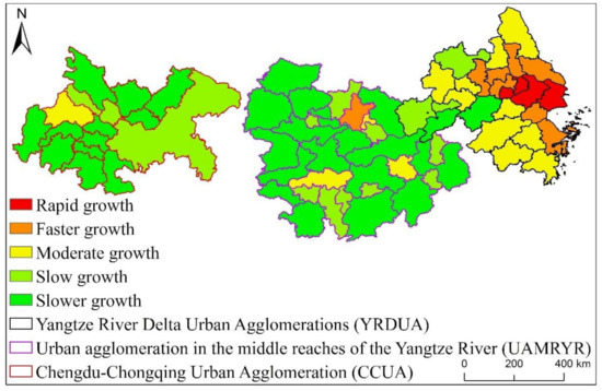
Figure 8.
EPC trend statistics of YREB’s three major urban agglomerations from 1992 to 2013.
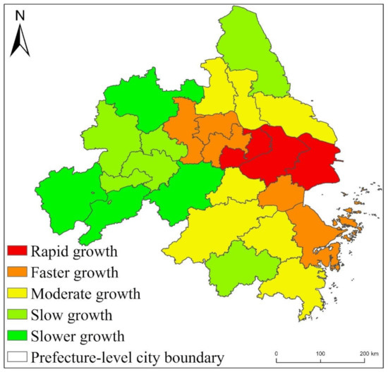
Figure 9.
Statistical chart of EPC change trend of YRDUA from 1992 to 2013.
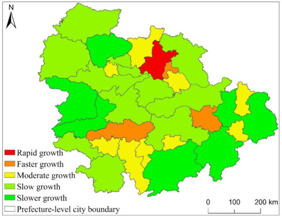
Figure 10.
Statistical chart of EPC change trend of UAMRYR from 1992 to 2013.
It can be seen from Figure 8 that from 1992 to 2013, the overall EPC increase of the three major urban agglomerations of YREB decreased from YRDUA in the east to UAMRYR in the middle and CCUA in the west. Moreover, the areas where the EPC growth rate is Rapid growth are all located in YRDUA. It can be seen that YRDUA is the area with the largest increase in EPC among the three major urban agglomerations of YREB. The EPC growth rate is the Faster growth area except UAMRYR’s Wuhan City, other areas are all located in YRDUA. Most of the regions where the EPC growth rate is Moderate growth are also located in YRDUA. The regions where the EPC growth rate of UAMRYR and CCUA are Moderate growth are all provincial capital cities. The increase in EPC is that the Slow growth and Slower growth areas are mostly located in UAMRYR and CCUA, reflecting the relatively small increase in EPC in these two urban agglomerations.
Specifically, as shown in Figure 9, within YRDUA, the cities with rapid growth in EPC are mainly Shanghai, Suzhou, Wuxi and Zhenjiang. With Shanghai as the core, these cities have highly developed economies and highly concentrated populations. They are also metropolitan areas. Therefore, the increase in EPC of these cities is not only the highest within YRDUA, but also the highest in the three major urban agglomerations of YREB. The areas where the EPC growth rate is Faster growth are mainly Nanjing, Zhenjiang and Changzhou in Jiangsu Province, Jiaxing, Ningbo and Zhoushan in Zhejiang Province. Some of these cities are the capital cities of their respective provinces and some are major cities. The economy of these cities is also very developed, the population size is also large, and the degree of urbanization is also high. Therefore, the growth rate of EPC is the second highest within YRDUA. The cities where the EPC growth rate is Moderate growth are Yangzhou, Taizhou and Nantong in Jiangsu Province, Hangzhou, Shaoxing and Taizhou in Zhejiang Province. These cities are also major cities in their respective provinces. The comprehensive development of these cities lags behind shanghai, suzhou, nanjing, etc., but it is obviously faster than the cities in the west of the YRDUA. Therefore, the EPC growth rate of these cities is Moderate growth in the YRDUA. The growth rate of EPC is slow growth and slower growth cities are mainly located in the west, south and north of YRDUA. The comprehensive development of these areas is relatively backward in YRDUA. Therefore, the growth rate of EPC is small.
From Figure 10, we can know that within UAMRYR, Wuhan is the only region that the EPC growth rate is rapid growth. It can be seen that Wuhan’s EPC growth rate is significantly higher than other cities. The areas where the EPC growth rate is faster growth are Changsha, Nanchang and Ezhou. Changsha City and Nanchang City are the capitals of Hunan Province and Jiangxi Province respectively. Therefore, the total economic aggregate, urban area and population scale of these two cities in their respective provinces are higher than those of other cities. Ezhou is close to Wuhan City, and is greatly affected by the radiation and driving of Wuhan City. Economic exchanges and interactions with Wuhan City are frequent. At the same time, the integration development process with Wuhan City is also very fast.
The regions where the EPC growth rate is moderate growth are other major cities in UAMRYR except for the provincial capital, such as Xiaogan City and Huangshi City in Hubei Province, Zhuzhou City and Xiangtan City in Hunan Province, and Yingtan City in Jiangxi Province. These cities are also relatively developed in their respective provinces. Therefore, the growth rate of EPC is Moderate growth. The areas where the EPC growth rate is slow growth and slower growth are mainly other cities in these provinces except for the capital cities and other major cities. The development of these prefectures and cities lags behind that of provincial capitals and other major prefectures, so the increase in EPC is the smallest.
It can be seen from Figure 11 that Chengdu is the only city within CCUA whose EPC growth rate is Rapid growth. This is because Chengdu is not only the core city of CCUA, but also the core city of Sichuan Province. Therefore, in terms of population, economic aggregate, and city size, they are all in the leading position within CCUA, so the increase in EPC is the most obvious. The EPC growth rate of Deyang City is faster growth. This is because Deyang City is not only close to Chengdu, but also within the radiation range of Chengdu. Therefore, Deyang City and Chengdu are closely connected, and the development of Deyang City is obviously affected by the radiation of Chengdu. As a result, the economy is relatively developed and urban development is constantly advancing, so the growth rate of EPC is only lower than that of Chengdu. The cities where the EPC growth rate is moderate growth are Chongqing City and Mianyang City, Suining City, Nanchong City, Guang’an City and Neijiang City in Sichuan Province. This is because although Chongqing has a leading position within CCUA in terms of economic aggregate, population size, and urban construction, as a municipality directly under the Central Government, Chongqing has a large area, and in addition to the main urban area, the overall development of most counties and cities is also Relatively backward, so the overall EPC increase in the end is not very obvious. The comprehensive development of Mianyang City, Suining City, Nanchong City, Guang’an City and Neijiang City in Sichuan Province lags behind the previous cities, so the increase in EPC is not obvious. The growth rates of EPC in Dazhou, Ziyang, Leshan, Yibin, Ya’an and Luzhou in Sichuan Province belong to slow growth and slower growth. The comprehensive development of these cities is in a backward position within CCUA, so the increase in EPC is also the smallest.
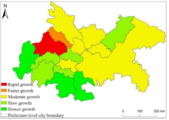
Figure 11.
Statistical chart of EPC change trend of CCUA from 1992 to 2013.
4.5. The Evolution Characteristics of the Spatial Pattern of the EPC of the Three Major Urban Agglomerations of YREB
From Table 1, Figure 12 and Figure 13, it can be found that from 1992 to 2013, the standard deviation ellipses of the three major urban agglomerations of YREB clearly showed an “east-west” spatial distribution characteristic, and the spatial directivity of YRDUA was very obvious. It shows that the driving force of YREBEPC’s growth is mainly from the growth of EPC in the east-west direction, and it also shows that YRDUA has the highest proportion of EPC in the three major urban agglomerations of YREB. In addition, we also found that the standard deviation ellipses of the three major urban agglomerations of YREB in the four years of 1992, 1999, 2006 and 2013 are almost all within the range of YRDUA and UAMRYR. It can be reflected that the core area of YREB’s EPC is in YRDUA, followed by UAMRYR, and CCUA has the lowest proportion. In addition, we also found that during the study period, the length of the major axis, the length of the minor axis, and the area of the standard deviation ellipse of the three major urban agglomerations of YREB have found certain changes. Specifically, the length of the major axis of the standard deviation ellipse increased from 657.87 km in 1992 to 696.90 km in 2013, an average annual increase of 1.77 km, and the length of the minor axis of the standard deviation ellipse increased from 173.89 km in 1992 to 199.43 km in 2013, an average annual increase of 1.16 km. The area of the standard deviation ellipse increased from 359,283.77 km2 in 1992 to 436,513.94 km2 in 2013, an average annual increase of 3510.46 km2. It can be seen that the driving force from the east-west direction of the three major urban agglomerations of YREB has a further growth trend, and the area of the standard deviation ellipse continues to increase, especially since the standard deviation ellipse in 2013 has begun to tilt toward CCUA. It can be seen that the proportion of EPC in the three major urban agglomerations of YREB is undergoing slight changes, especially the proportion of EPC in CCUA is slowly increasing.

Table 1.
Statistical table of the standard deviation ellipse data of the three major urban agglomerations of YREB in 1992–2013.
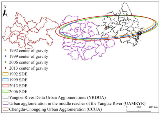
Figure 12.
EPC standard deviation ellipse and average center of gravity distribution of the three major urban agglomerations of YREB from 1992 to 2013.
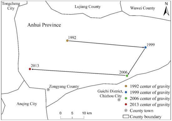
Figure 13.
The distribution of the average center of gravity movement trajectory of the three major urban agglomerations of YREB from 1992 to 2013.
In terms of center of gravity migration, the center of gravity of the EPC of YREB’s three major urban agglomerations shows the characteristics of moving from west to east, and then from east to west, but the magnitude of the movement is relatively small. The center of gravity of EPC in the four years of 1992, 1999, 2006 and 2013 is located in Zongyang County, Anhui Province, that is, within the scope of YRDUA, and is also close to the regional scope of UAMRYR. Therefore, we can find that YRDUA has the highest proportion of EPC among the three major urban agglomerations of YREB, followed by UAMRYR, and CCUA has the smallest proportion. In terms of the comparison of the moving distance of the EPC center of gravity, the moving distance was the largest from 2006 to 2013, followed by the moving distance from 1992 to 1999, and the moving distance from 1999 to 2006 was the smallest. It can be seen that during the study period, the EPC of YREB’s three major urban agglomerations has increased significantly. Among them, YRDUA has the largest increase, followed by UAMRYR, and CCUA has the smallest increase. In general, due to the obvious gaps between the three major urban agglomerations of YREB in terms of urban scale, total economic volume, and population, the spatial distribution pattern of the overall EPC of the three major urban agglomerations of YREB remains unchanged.
4.6. Spatial Autocorrelation Analysis of EPC of YREB’s Three Major Urban Agglomerations
In order to better discover the spatial autocorrelation features and structural change characteristics of the EPC within the three major urban agglomerations of YREB. Therefore, this paper combines the global Moran’s I index, the local Moran scatter plot and LISA to monitor the spatial agglomeration and local spatial instability of the EPC of the three major urban agglomerations of YREB. The specific calculation results were shown in Table 2, Figure 13 and Figure 14.
Table 2.
EPC global Moran’s I index statistics for the three major urban agglomerations of YREB from 1992 to 2013.
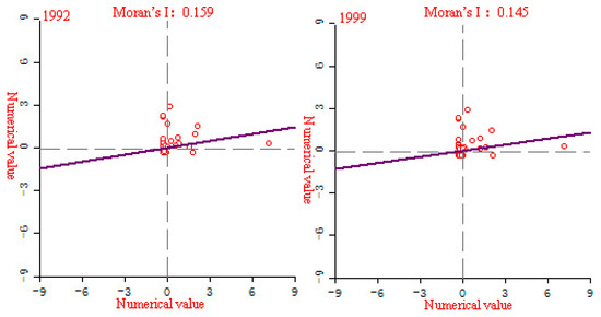
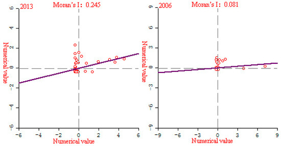
Figure 14.
EPC partial Moran’slocal Moran’s I index scatter plot of YREB’s three major urban agglomerations in 1992–2013.
According to Table 2, during the research period, the Moran’s I index of the EPC of the three major urban agglomerations of YREB is between −1 and +1, and has been increasing. Specifically, it increased from 0.58 in 1992 to 0.77 in 2013, with an average annual increase of 1.49%, and the value of Moran’s I index is getting closer to 1. The Z value increased from 6251.27 in 1992 to 8208.36 in 2013, with an average annual increase of 1.44%, and the Z value has been increasing. In addition, we also found that the p-value is always less than 0.001. It can be seen that the EPC of YREB’s three major urban agglomerations is statistically significant and has obvious correlation, and with the increase of time, the correlation of the EPC of YREB’s three major urban agglomerations becomes more and more significant.
Figure 14 shows the local Moran’s I index scatter plot of the EPC of YREB three major urban agglomerations in 1992–2013. We can clearly find that with the change of time, the agglomeration of red points (number of samples) in the three major urban agglomerations of YREB has become more and more obvious. Among them, the degree of agglomeration was the highest in 2013, and the slope of the line was getting bigger and bigger, especially in 2013, the slope of the line was significantly greater than in 1992, 1999 and 2006. It clearly reflects that the spatial correlation of the EPC of YREB provinces and cities has been continuously enhanced, which is consistent with the calculation results of the global Moran’s I index, indicating that with the increase of time, the spatial correlation of the EPC of the three major urban agglomerations of YREB has become more and more obvious.
The LISA cluster map of YREB’s three major urban agglomerations from 1992 to 2013 is shown in Figure 15. We can clearly find that with the change of time, the spatial correlation and agglomeration of the three major urban agglomerations of YREB has increased significantly. From 1992 to 2013, the number of spatial autocorrelation agglomerations of the three major urban agglomerations of YREB increased from 7 to 16, and the degree of agglomeration increased significantly. Specifically, the cities where EPC presents “High-High” clusters are all located in YRDUA, especially Shanghai, the southeast of Jiangsu Province, and the north and east of Zhejiang Province. These cities are among the most economically developed regions in China. The cities are large in scale, highly concentrated in population, highly developed economy, and highly integrated. Therefore, the largest number of EPC within the three urban agglomerations of YREB have been produced and the degree of agglomeration is also high. The cities where EPC presents “Low-Low” clusters are mainly distributed in UAMRYR and CCUA. Compared with YRDUA in the east, the comprehensive development of these cities is far behind. Therefore, the EPC produced is relatively small and the degree of agglomeration is relatively low. EPC shows that the “Low-High” clusters of cities are all located in YRDUA in the east of YREB’s three major urban agglomerations. The comprehensive development of these cities only lags behind YRDUA’s most developed cities. Therefore, the urban scale, total economic volume, and population size are relatively high, which has resulted in a larger EPC and a certain degree of agglomeration.
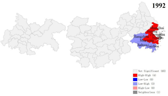
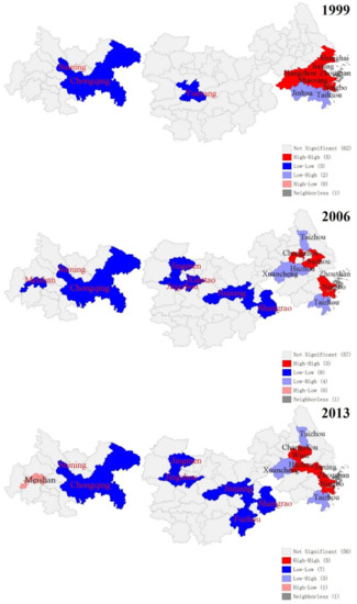
Figure 15.
The LISA cluster map of the EPC of YREB’s three major urban agglomerations in 1992–2013.
4.7. Spatial-Temporal Difference Analysis of Influencing Factors of EPC in Three Urban Agglomerations in the Yreb Based on GWR
Table 3 shows the GWR model estimation results of the EPC of the three major urban agglomerations in the YREB, and the regression fitting coefficient also shows a gradually increasing trend. The R2 values of the three years 1999, 2006, and 2013 are 0.761, 0.788, and 0.803 respectively, reflecting the good fitting performance of the GWR model. Based on the GWR model, it can reflect 73.20%, 75.10%, and 77.10% of the temporal and spatial changes in EPC of the three major urban agglomerations in the YREB in 1999, 2006, and 2013. Therefore, it can better meet the research needs and has high reliability.
Table 3.
GWR model estimation results.
According to the box plot of the GWR model regression coefficient distribution of the EPC of the three major urban agglomerations in the YREB in 1999 (Figure 16), it can be seen that the regression coefficients of the proportion of secondary industry in GDP, GDP per capita, urbanization rate, per capita disposable income of urban residents and annual sunshine hours are all positive. It directly reflects that these five influencing factors have a positive impact on the EPC of the three major urban agglomerations in the YREB in 1999. Specifically, the regression coefficient of Per capita disposable income of urban residents has the largest mean value, indicating that Per capita disposable income of urban residents has the greatest impact on EPC. At the same time, the regression coefficient of Per capita disposable income of urban residents has the largest distribution range, indicating the spatial difference is the most obvious. Both the mean value and the distribution interval of the regression coefficients of annual sunshine hours are in the second position, which not only shows that the annual sunshine hours has a greater impact on EPC, but also shows that the regression coefficients of the annual sunshine hours have obvious spatial differences. The mean value and distribution interval of the regression coefficients of the other three influencing factors are relatively close, indicating that the degree of influence of these three influencing factors on EPC is close to the spatial difference of the regression coefficient.
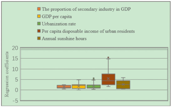
Figure 16.
Box plot of GWR model regression coefficient distribution of EPC in the three major urban agglomerations of the YREB in 1999.
From the distribution box plot of the GWR model regression coefficients of the three major urban agglomerations in the YREB in 2006 (Figure 17), it can be seen that the regression coefficients of the proportion of secondary industry in GDP, GDP per capita, urbanization rate, per capita disposable income of urban residents, annual sunshine hours are all positive as in 1999. It directly reflects that these five influencing factors have a positive impact on the EPC of the three major urban agglomerations in the YREB in 2006. Specifically, the regression coefficients of annual sunshine hours have the largest distribution range, indicating that their spatial differences are the most obvious. At the same time, the average value of annual sunshine hours is also in the second position, which also indicates that it has a greater impact on EPC. The regression coefficient of per capita disposable income of urban residents has the largest mean value, which directly shows that per capita disposable income of urban residents has the greatest impact on EPC. The proportion of secondary industry in GDP’s regression coefficient is in the second position, which also shows that its spatial difference is more obvious. The regression coefficients of GDP per capita and urbanization rate are relatively close, which directly indicates that the impact of these two influencing factors on EPC is relatively close, and the distribution range of the regression coefficient of urbanization rate is greater than that of GDP per capita. The distribution interval of the urbanization rate indicates that the spatial difference of the regression coefficient of urbanization rate is more obvious.
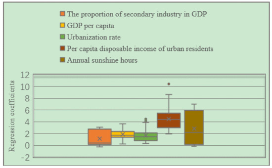
Figure 17.
Box plot of GWR model regression coefficient distribution of EPC in the three major urban agglomerations of the YREB in 2006.
From the box plot of the GWR model regression coefficient distribution of EPC in the three major urban agglomerations in the YREB in 2013 (Figure 18), it can be seen that the regression coefficients of GDP per capita, urbanization rate, per capita disposable income of urban residents, annual sunshine hours are all positive. It directly reflects that these four influencing factors have a positive impact on the EPC of the three major urban agglomerations in the YREB in 2006. Specifically, the regression coefficient of per capita disposable income of urban residents has the largest mean value, indicating that it has the greatest impact on EPC. At the same time, the distribution interval of the regression coefficient of per capita disposable income of urban residents is also in the second position, which also shows that the spatial difference is also more obvious. The regression coefficient of annual sunshine hours have the longest distribution interval, which directly shows that its spatial difference is the most obvious. At the same time, the mean value of the regression coefficient of Annual sunshine hours is also in the second position, indicating that its impact on EPC is also greater. The regression coefficients of the two influencing factors of GDP per capita and urbanization rate are relatively close, which directly shows that the impact of these two influencing factors on EPC is relatively close, and the distribution range of the regression coefficient of Urbanization rate is greater than that of GDP per capita. The distribution interval of the urbanization rate indicates that the spatial difference of the regression coefficient of urbanization rate is more obvious. The regression coefficient of the proportion of secondary industry in GDP is negative, indicating that the proportion of secondary industry in GDP has an inhibitory effect on EPC. At the same time, the regression coefficient of the proportion of secondary industry in GDP has a longer distribution range, indicating that the spatial difference is also more obvious.
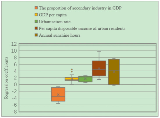
Figure 18.
Box plot of GWR model regression coefficient distribution of EPC in the three major urban agglomerations of the YREB in 2013.
In order to find the spatial distribution characteristics of the regression coefficients of the proportion of secondary industry in GDP, per capital, urbanization rate, per capital disposable income of urban residents and annual sunshine hours of the three major urban agglomerations in the YREB in 1999, 2006 and 2013 more intuitively and concretely. We also draw the spatial distribution of the regression coefficients of these five factors, as shown in Figure 19, Figure 20 and Figure 21.
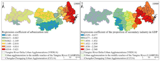
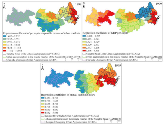
Figure 19.
The spatial distribution map of the regression coefficients of the GWR model influencing factors of EPC in the three major urban agglomerations of the YREB in 1999.
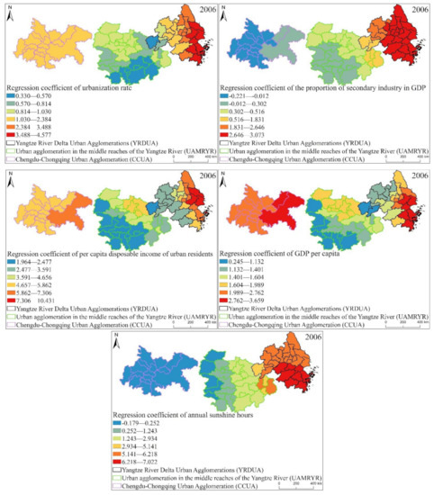
Figure 20.
The spatial distribution map of the regression coefficients of the GWR model influencing factors of EPC in the three major urban agglomerations of the YREB in 2006.
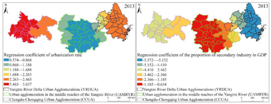
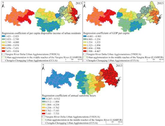
Figure 21.
The spatial distribution map of the regression coefficients of the GWR model in fluencing factors of EPC in the three major urban agglomerations of the YREB in 2013.
It can be found from Figure 19 that the proportion of secondary industry in GDP, GDP per capital, urbanization rate, per capital disposable income of urban residents of the three major urban agglomerations in the YREB in 1999, the regression coefficients of annual sunshine hours are similar in spatial distribution. On the whole, the regression coefficients are decreasing from the YRDUA to UAMRYR and CCUA. This also directly reflects that the impact of these five influencing factors is the largest in the YRDUA, followed by UAMRYR, and CCUA has the least. Specifically, the distribution characteristics of the regression coefficient of urbanization rate are the most obvious. The highest value is concentrated in the coastal areas of the YRDUA, reflecting that the EPC in these areas is most obviously affected by the urbanization rate. The highest value of the regression coefficient of the proportion of secondary industry in GDP is concentrated in the cities at the junction of the YRDUA and UAMRYR. This is due to the accompanying Chinese government’s call for industrial transfer. Therefore, the cities at the junction of the YRDUA and UAMRYR have undertaken labor-intensive industries and heavy industries from the coastal areas of the YRDUA. Therefore, it will naturally produce high EP.
The highest value of regression coefficient of per capita disposable income of urban residents is also concentrated in the coastal cities of the YRDUA, while the second highest value appears in the Wuhan urban agglomeration in the UAMRYR. This is because the Wuhan urban agglomeration is the core city of UAMRY, which has rapid comprehensive development and relatively high residents’ income. Therefore, it finally appeared that the EPC of the Wuhan city agglomeration was significantly affected by per capita disposable income of urban residents. The spatial distribution of the regression coefficient of GDP per capita also has a new high-value area, namely Chongqing City. This is because Chongqing, as the only municipality directly under the Central Government in western my country, is the core city of CCUA, and its comprehensive development is relatively fast. Therefore, GDP per capita has a significant impact on Chongqing’s EPC. The high-value areas of the Regression coefficient of annual sunshine hours are the southern part of YRDUA and the junction area between the YRDUA and UAMRYR. Most of these cities are located to the south and are close to the coast. Therefore, it is most affected by annual sunshine hours.
It can be found from Figure 20 that the spatial distribution of the regression coefficients of the proportion of secondary industry in GDP, GDP per capital, urbanization rate, per capital disposable income of urban residents and annual sunshine hours of the three urban agglomerations in the YREB in 2006 is similar to that in 1999. On the whole, the regression coefficient decreases from YRDUA to UAMRYR and CCUA. This also directly reflects that YRDUA is the most affected by these five influencing factors, followed by UAMRYR and CCUA. Specifically, the high-value areas of the regression coefficient of urbanization rate and the proportion of secondary industry in GDP are concentrated in the YRDUA. This is because the YRDUA is the most developed city in the YREB, and the values of urbanization rate and the proportion of secondary industry in GDP are the highest within the three major urban agglomerations in the YREB. Therefore, these two factors have the most obvious impact on EPC.
The high values of regression coefficient of per capita disposable income of urban residents and regression coefficient of GDP per capita are not only distributed in the YRDUA, but also in the CCUA in the west. This is because the Chinese government implemented the “Western Development Plan” in 2006, focused on promoting the development of Chongqing and Chengdu, including the CCUA in the west. Therefore, the residents’ income and GDP per capita of the CCUA have been significantly developed, and therefore have become the main factors affecting EPC. The high-value areas of the regression coefficient of annual sunshine hours are mainly concentrated in the YRDUA, because the YRDUA is the urban agglomeration with the highest degree of urbanization among the three major urban agglomerations in the YREB. At the same time, it is located in coastal areas and has obvious urban heat island effects. Therefore, annual sunshine hours is the main factor influencing EPC.
It can be found from Figure 21 that the spatial distribution characteristics of the regression coefficients of the proportion of secondary industry in GDP, GDP per capital, urbanization rate, per capital disposable income of urban residents and annual sunshine hours of the three major urban agglomerations in the YREB in 2013 have changed compared with those in 1999 and 2006. Specifically, regression coefficient of urbanization rate, regression coefficient of the proportion of secondary industry in GDP, regression coefficient of per capita disposable income of urban residents, The high values of regression coefficient of GDP per capita are obviously concentrated in the UAMRYR and CCUA in the western part. It clearly reflects that in 2013, the urbanization rate, the proportion of secondary industry in GDP, per capita disposable income of urban residents, and GDP per capita in the CCUA and UAMRYR have increased significantly. Therefore, the influence of these four values on the EPC of the CCUA and UAMRYR is more obvious within the three urban agglomerations in the YREB. The cities with high values of regression coefficient of annual sunshine hours have increased from the YRDUA to the eastern cities in the UAMRYR. It directly reflects the increase in annual sunshine hours in these cities, leading to an increase in temperature. Eventually, the appearance of annual sunshine hours in these cities has a significant impact on EPC.
4.8. Analysis of the Importance of Factors Affecting EPC in the Three Major Urban Agglomerations in the YREB Based on Random Forest Algorithm
Based on the random forest algorithm, the statistics of the importance scores of the three major urban agglomerations in the YREB in 1999, 2006, and 2013 are shown in Table 4. According to the importance scores of different influencing factors, we can clearly find that in 1999, the main influencing factors of EPC in the three major urban agglomerations in the YREB were the proportion of secondary industry in GDP, GDP per capita, and urbanization rate. In 2006, the main influencing factors of EPC in the three major urban agglomerations in the YREB were per capita disposable income of urban residents, the proportion of secondary industry in GDP, and urbanization rate. In 2013, the main influencing factors of EPC in the three major urban agglomerations in the YREB were the proportion of secondary industry in GDP, per capita disposable income of urban residents, and average annual temperature. Through a comprehensive analysis of the three years of 1999, 2006, and 2013, we found that the main influencing factors of EPC in the three major urban agglomerations in the YREB are the proportion of secondary industry in GDP, per capita disposable income of urban residents, and urbanization rate.
Table 4.
Statistical table of the importance scores of the influencing factors of EPC of the three major city clusters in the YREB in 1999, 2006, and 2013.
In order to make the importance scores of the influencing factors of EPC in 1999, 2006 and 2013 based on the random forest algorithm of the YREB more intuitive and specific, we draw a histogram, and the specific content is shown in Figure 22. At the overall level, the importance scores of the 12 factors influencing the EPC of the three major urban agglomerations in the YREB selected in this paper are roughly similar in the three years of 1999, 2006, and 2013. The top three influencing factors with the highest total score in the three years are the proportion of secondary industry in GDP, per capita disposable income of urban residents, and urbanization rate, in order of the highest score. It directly reflects that these three influencing factors have the most obvious impact on EPC in the YREB. This is because the secondary industry is mainly based on heavy industry. Therefore, it will inevitably produce a large EPC. Therefore, the proportion of secondary industry in GDP is directly correlated with EPC. Per capita disposable income of urban residents and urbanization rate directly represents the income that residents spend on consumption and the number of urban population, so they also have a close positive correlation with EPC.
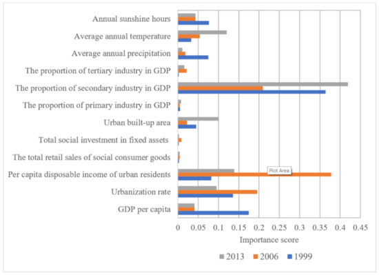
Figure 22.
Statistics of the importance scores of EPC influencing factors of the three major urban agglomerations in the YREB in 1999, 2006, and 2013.
Specifically, in 1999, the main influencing factors of EPC in the three major urban agglomerations in the YREB were the proportion of secondary industry in GDP, GDP per capita, and Urbanization rate. This is because the development of the secondary industry is still one of the main industries, which leads to the most obvious EPC. In 2006, the main influencing factors of EPC in the three major urban agglomerations in the YREB were per capita disposable income of urban residents, the proportion of secondary industry in GDP, and urbanization rate. This is because with the continuous development of the three major urban agglomerations in the YREB, per capita disposable income of urban residents has increased significantly, which means that residents have enough income to use electricity resources. In 2013, the main influencing factors of EPC in the three major urban agglomerations in the YREB were the proportion of secondary industry in GDP, per capita disposable income of urban residents, and average annual temperature. This is because with the industrial transfer of the exhibition held by the Chinese government, some heavy industries and labor-intensive industries included in the secondary industry began to transfer from coastal areas to the vast urban agglomerations in the UAMRYR and CCUA. Then these industries became the main force for the development of the UAMRYR and CCUA.
5. Discussions and Conclusions
5.1. Discussions
YREB spans the three major regions of China’s east, middle and west, and is one of the “three national strategies” implemented by the Chinese government. It includes three national-level urban agglomerations, YRDUA, UAMRYR and CCUA, which is the key to the development of YREB, especially YRDUA is the key to YREB development, but these three urban agglomerations still have obvious differences in all aspects. Electricity, as a very important element in the development of modern human society, is one of the important basic elements for the continuous development of modern human civilization. Therefore, this paper conducts a comparative analysis of the Spatio-temporal Dynamic Evolution Characteristics and Influencing factors of the EPC of YREB’s three major urban agglomerations from 1992 to 2013. The research work of this paper has certain significance and value for realizing the sustainable development of YREB three urban agglomerations and the optimal allocation of electricity resources.
Compared with previous studies, this paper selects the three major urban agglomerations of YREB as the research object. The research methods used in this paper are also more comprehensive and richer, and the findings from comparative analysis are more meaningful. However, due to the relatively low resolution of DMSP/OLS night light data, the EPC estimation effect for small villages and towns needs to be improved. Therefore, in our follow-up research, DMSP/OLS night light data will be merged with higher resolution NPP-VIIRS night light data and Luojia01 night light data (or using NPP-VIIRS night light data and Luojia01 night light data alone) to further clarify our results.
5.2. Conclusions
In this paper, based on the EPC data extracted from DMSP/OLS night light data, we select the three major urban agglomerations of YREB as the research object. Next, we used coefficient of variation, kernel density analysis, cold hot spot analysis, trend analysis, standard deviation ellipse and Moran’s I Index method to analyze and compare the EPC spatiotemporal evolution dynamic characteristics of the three major urban agglomerations of YREB. In addition, we also use the geographically weighted regression (GWR) model and Random forest algorithm to analyze the influencing factors of the EPC of the three major urban agglomerations in the YREB.
The conclusions we got are as follows: (1) From 1992 to 2013, the overall CV of EPC of YREB’s three urban agglomerations has been in a downward trend. The coefficient of variation (CV) dropped from 8.08 in 1992 to 2.98 in 2013, with an average annual decrease of −2.87%, reflecting that the EPC differences within the three major urban agglomerations of YREB are gradually decreasing. (2) During the study period, the EPC of YREB’s three major urban agglomerations is in an increasing trend, and the distribution of EPC values also decreases from YRDUA in the east to UAMRYR in the middle and CCUA in the west. (3) With the increase of time, the accumulation of hot and cold EPCs in the three major urban agglomerations of YREB has become more and more obvious, and the distribution of high-value areas of EPC hotspots also obviously shows a decreasing characteristic from RDUA to UAMRYR and CCUA. (4) From 1992 to 2013, the overall EPC growth rate of YREB’s three major urban agglomerations has decreased from YRDUA in the east to UAMRYR in the middle and CCUA in the west. The rapid growth of EPC is located in YRDUA. (5) The standard deviation ellipses of the EPC of YREB’s three major urban agglomerations clearly show the “east-west” spatial distribution characteristics, and the spatial directivity of YRDUA is very obvious. In terms of the center of gravity migration, the center of gravity of YREB’s EPC as a whole shows the characteristics of moving from west to east, and then from east to west. (6) During the study period, the EPC of the three major urban agglomerations of YREB is statistically significant and has obvious correlation. And with the increase of time, the relevance of the EPC of YREB’s three major urban agglomerations becomes more and more significant. With the change of time, the agglomeration of EPC in the three major cities of YREB has become more and more obvious. (7) By using the GWR model, we found that the five influencing factors we selected basically have a positive impact on the EPC of the YREB through the use of the GWR model. In addition, we also found that the numerical value of the regression coefficients of these five influencing factors also basically showed the characteristics of decreasing from the YRDUA to the UAMRYR and CCUA. (8) By using the random forest algorithm, we found that the three main influencing factors of EPC in the three major urban agglomerations in the YREB are the proportion of secondary industry in GDP, per capita disposable income of urban residents, and urbanization rate.
Author Contributions
Writing—original draft preparation, Y.Z.; writing—review and editing, A.L. and C.X.; participate in data processing and analysis, Z.Z. All authors have read and agreed to the published version of the manuscript.
Funding
This research was supported by the National Social Science Foundation of China (Research on Benefit Compensation Mechanism for Promoting Regional Coordinated Development in the New Era (18ZDA040)).
Institutional Review Board Statement
Not applicable.
Informed Consent Statement
Informed consent was obtained from all subjects involved in the study.
Data Availability Statement
The data used in this paper can be downloaded from the National Earth System Science Data Center (http://www.geodata.cn/).
Conflicts of Interest
The authors declare no conflict of interest.
References
- Cao, X.F.; Yang, G.Y.; Song, M.L. Research on Influencing Factors of Power Energy Efficiency in China. Sci. Decis. 2011, 17, 76–93. (In Chinese) [Google Scholar]
- Wu, J.; Tang, L. Research on the Influencing Factors of Provincial Power Intensity in china—Based on the Analysis of Spatial Metrology Model. Price Theory Pract. 2020, 40, 53–56. (In Chinese) [Google Scholar]
- Xie, Y.H.; Weng, Q.H. Detecting urban-scale dynamics of electricity consumption at Chinese cities using time-series DMSP-OLS (Defense Meteorological Satellite Program-Operational Linescan System) nighttime light imageries. Energy 2016, 100, 177–189. [Google Scholar] [CrossRef]
- Cao, X.; Wang, J.M.; Chen, J.; Shi, F. Spatialization of electricity consumption of China using saturation-corrected DMSP-OLS data. Int. J. Appl. Earth Obs. Geoinf. 2014, 28, 193–200. [Google Scholar] [CrossRef]
- Chand, T.R.K.; Badarinath, K.V.S.; Elvidge, C.D.; Tuttle, B.T. Spatial characterization of electrical power consumption patterns over India using temporal DMSP-OLS night-time satellite data. Int. J. Remote Sens. 2009, 30, 647–661. [Google Scholar] [CrossRef]
- Jia, R.X.; Liu, Y. Research on optimization of China's power resource structure and spatial layout. Resour. Sci. 2003, 25, 14–19. (In Chinese) [Google Scholar]
- Zhao, N.Z.; Ghosh, T.; Samson, E.L. Mapping spatiotemporal changes of Chinese electric power consumption using night-time imagery. Int. J. Remote Sens. 2012, 20, 20–6320. [Google Scholar]
- Bao, C.; Liu, R.W. Electricity Consumption Changes across China’s Provinces Using A Spatial Shift-Share Decomposition Model. Sustainability 2019, 11, 1–15. [Google Scholar]
- He, C.Y.; Ma, Q.; Li, T.; Yang, Y.; Liu, Z.F. Spatiotemporal dynamics of electric power consumption in Chinese Mainland from 1995 to 2008 modeled using DMSP/OLS stable nighttime lights data. J. Geogr. Sci. 2012, 22, 125–136. [Google Scholar] [CrossRef]
- He, C.Y.; Ma, Q.; Liu, Z.F.; Zhang, Q.F. Modeling the spatiotemporal dynamics of electric power consumption in Mainland China using saturation corrected DMSP/OLS nighttime stable light data. Int. J. Digit. Earth 2014, 7, 993–1014. [Google Scholar] [CrossRef]
- Deng, C.B.; Lin, W.Y.; Chen, S.L. Use of smart meter readings and nighttime light images to track pixel-level electricity consumption. Remote Sens. Lett. 2019, 10, 205–213. [Google Scholar] [CrossRef]
- Yang, X.C.; Kang, L.L.; Zhang, B.; Ji, C.X. Electricity consumption estimation and influencing factors analysis based on multi-source remote sensing information—Taking Zhejiang Province as an example. Geogr. Sci. 2013, 33, 718–723. (In Chinese) [Google Scholar]
- Pan, J.H.; Li, J.F. Spatiotemporal Dynamics of Electricity Consumption in China. Appl. Spat. Anal. Policy 2019, 12, 395–422. [Google Scholar] [CrossRef]
- Elvidge, C.D.; Cinzano, P.; Pet, D.R. The nights at mission concept. Int. J. Remote Sens. 2007, 8, 2645–2670. [Google Scholar] [CrossRef]
- Huang, X.M.; Schneider, A.; Friedl, M.A. Mapping sub-pixel urban expansion in China using MODIS and DMSP/OLS nighttime lights. Remote Sens. Environ. 2016, 175, 92–108. [Google Scholar] [CrossRef]
- Ma, T.; Zhou, Y.K.; Zhou, C.H.; Pei, T.; Xu, T. Night-time light derived estimation of spatio-temporal characteristics of urbanization dynamics using DMSP/OLS satellite data. Remote Sens. Environ. 2015, 158, 453–464. [Google Scholar] [CrossRef]
- Zhang, X.X.; Guo, S.; Guan, Y.N.; Cai, D.L.; Zhang, C.Y.; Fraedrich, K.; Xiao, H.; Tian, Z.Z. Urbanization and Spillover Effect for Three Megaregions in China: Evidence from DMSP/OLS Nighttime Lights. Remote Sens. 2018, 10, 1–16. [Google Scholar] [CrossRef]
- Chen, X.; Peng, J.; Liu, Y.X.; Chen, Y.Q.; Li, T.D. Measurement of urban spatial expansion and spatial correlation in Beijing-Tianjin-Hebei region based on DMSP/OLS night light data. Geogr. Res. 2018, 37, 898–909. [Google Scholar]
- Li, C.; Li, G.E.; Zhu, Y.J.; Ge, Y.; Kung, H.T.; Wu, Y.J. A likelihood-based spatial statistical transformation model (LBSSTM) of regional economic development using DMSP/OLS time-series nighttime light imagery. Spatial Statistics. Spat. Stat. 2017, 21, 421–439. [Google Scholar] [CrossRef]
- Fu, H.Y.; Shao, Z.F.; Fu, P.; Cheng, Q.M. The Dynamic Analysis between Urban Nighttime Economy and Urbanization Using the DMSP/OLS Nighttime Light Data in China from 1992 to 2012. Remote Sens. 2017, 9, 1–19. [Google Scholar] [CrossRef]
- Qi, K.; Hu, Y.N.; Cheng, C.Q.; Chen, B. Transferability of Economy Estimation Based on DMSP/OLS Night-Time Light. Remote Sens. 2017, 9, 1–13. [Google Scholar] [CrossRef]
- Wang, J.H.; Zhang, Y.B.; Yi, G.H.; Bie, X.J.; Liu, D.; Zhang, T.T. Spatial analysis of Sichuan GDP based on DMSP/OLS night light data. Surv. Mapp. Sci. 2019, 44, 50–60. (In Chinese) [Google Scholar]
- Lv, Q.; Liu, H.B.; Wang. J., T.; Liu., H.; Shang, Y. Multiscale analysis on spatiotemporal dynamics of energy consumption CO2 emissions in China: Utilizing the integrated of DMSP-OLS and NPPVIIRS nighttime light datasets. Sci. Total Environ. 2020, 703, 1–12. (In Chinese) [Google Scholar] [CrossRef]
- Yue, Y.L.; Tian, L.; Yue, Q.; Wang, Z. Spatiotemporal Variations in Energy Consumption and Their Influencing Factors in China Based on the Integration of the DMSP-OLS and NPP-VIIRS Nighttime Light Datasets. Remote Sens. 2020, 12, 1–23. [Google Scholar] [CrossRef]
- Zhang, X.W.; Wu, J.S.; Peng, J.; Cao, Q.W. The Uncertainty of Nighttime Light Data in Estimating Carbon Dioxide Emissions in China: A Comparison between DMSP-OLS and NPP-VIIRS. Remotesensing 2017, 12, 1–20. [Google Scholar] [CrossRef]
- Zhang, Y.N.; Pan, J.H. Spatiotemporal simulation and differentiation pattern of China's carbon emissions based on DMSP/OLS data. China Environ. Sci. 2019, 39, 1436–1446. [Google Scholar]
- Huang, Q.X.; Yang, Y.; Li, Y.J.; Gao, B. A Simulation Study on the Urban Population of China Based on Nighttime Light Data Acquired from DMSP/OLS. Sustainability 2016, 8, 1–13. [Google Scholar] [CrossRef]
- Sun, W.C.; Zhang, X.; Wang, N.; Cen, Y. Estimating Population Density Using DMSP-OLS Night-Time Imagery and Land Cover Data. IEEE J. Sel. Top. Appl. Earth Obs. Remote Sens. 2017, 10, 2674–2684. [Google Scholar] [CrossRef]
- Yu, S.S.; Zhang, Z.X.; Liu, F. Monitoring Population Evolution in China Using Time-Series DMSP/OLS Nightlight Imagery. Remote Sens. 2018, 10, 1–21. [Google Scholar] [CrossRef]
- Chen, Q.; Hou, X.Y. Integrate land use data and night light data to optimize population spatialization model. J. Geo-Inf. Sci. 2015, 17, 1370–1377. (In Chinese) [Google Scholar]
- Ma, Z.Y.; Xiao, H.W. Study on my country's Provincial Power Consumption Simulation Based on Satellite Light Data. 2017, 39, 6–14. (In Chinese) [Google Scholar]
- Hu, T.; Huang, X. A novel locally adaptive method for modeling the spatiotemporal dynamics of global electric power consumption based on DMSP-OLS nighttime stable light data. Appl. Energy 2019, 240, 778–792. [Google Scholar] [CrossRef]
- Zhu, Y.G.; Xu, D.Y.; Ali, S.H.; Ma, R.Y.; Cheng, J.H. Can Nighttime Light Data Be Used to Estimate Electric Power Consumption? New Evidence from Causal-Effect Inference. Energies 2019, 12, 1–14. [Google Scholar] [CrossRef]
- Husi, L.; Masanao, H.; Hiroshi, Y.; Kazuhiro, N.; Gegen, T.; Fumihiko, N.; Okada, S. Estimating energy consumption from night-time DMPS/OLS imagery after correcting for saturation effects. Int. J. Remote Sens. 2010, 16, 4443–4458. [Google Scholar]
- Shi, K.F.; Yu, B.L.; Huang, C.; Wu, J.P.; Sun, X. Exploring spatiotemporal patterns of electric power consumption in countries along the Belt and Road. Energy 2018, 150, 847–859. (In Chinese) [Google Scholar] [CrossRef]
- Cowan, W.N.; Chang, T.Y.; Roula, I.L.; Rangan, G. The nexus of electricity consumption, economic growth and CO2 emissions in the BRICS countries. Energy Policy. 2014, 66, 359–368. [Google Scholar] [CrossRef]
- Zhu, J.; Zhao, Z.Y. Chinese Electric Power Development Coordination Analysis on Resource, Production and Consumption:A Provincial Case Study. Sustainability 2017, 9, 1019. [Google Scholar] [CrossRef]
- Li, S.Y.; Cheng, L.; Liu, X.P.; Mao, J.Y.; Wu, J.; Li, M.C. City type-oriented modeling electric power consumption in China using NPP-VIIRS nighttime stable light data. Energy 2019, 189, 1–12. [Google Scholar] [CrossRef]
- Shi, K.F.; Yu, B.L.; Huang, Y.X.; Hu, Y.J.; Yin, B.; Chen, Z.Q.; Chen, L.J.; Wu, J.P. Evaluating the Ability of NPP-VIIRS Nighttime Light Data to Estimate the Gross Domestic Product and the Electric Power Consumption of China at Multiple Scales: A Comparison with DMSP-OLS Data. Remote Sens. 2014, 6, 1–20. [Google Scholar] [CrossRef]
- Lin, J.; Shi, W.Z. Statistical Correlation between Monthly Electric Power Consumption and VIIRS Nighttime Light. Isprs Int. J. Geo-Inf. 2020, 9, 1–13. [Google Scholar] [CrossRef]
- Pan, J.H.; Li, J.F. China’s electricity consumption estimation and temporal dynamics based on night light images. Geogr. Res. 2016, 35, 627–638. [Google Scholar]
- Sumana, S.; Prasun, K.G.; Srivastav, S.K. Comparative analysis between VIIRS-DNB and DMSP-OLS night-time light data to estimate electric power consumption in Uttar Pradesh, India. Int. J. Remote Sens. 2020, 41, 2565–2580. [Google Scholar]
- Arati, P.; Bhuvanesh, V.; Debasish, C. Estimating electrification using multi-temporal DMSP/OLS night imagery as proxy measure of human well-being in India. Spat. Inf. Res. 2020, 28, 469–473. [Google Scholar]
- Bismay, R.T.; Haroon, S.; Elvidge, C.D.; Yu, T.; Prem, C.P.; Meenu, R.I.; Pavan, K. Modeling of Electric Demand for Sustainable Energy and Management in India Using Spatio-Temporal DMSP-OLS NightTime Data. Environ. Manag. 2018, 61, 615–623. [Google Scholar]
- Tomasz, J. Modeling electricity consumption using nighttime light images and artificial neural networks. Energy 2019, 179, 831–842. [Google Scholar]
- Alexander, C.; Bruce, T.D.A. The use of nighttime lights satellite imagery as a measure of Australia's regional electricity consumption and population distribution. Int. J. Remote Sens. 2019, 31, 4459–4480. [Google Scholar]
- Lin, J.T.; Shi, W.Z. Improved Denoising of VIIRS Nighttime Light Imagery for Estimating Electric Power Consumption. Ieee Geosci. Remote Sens. Lett. 2020, 17, 1782–1786. [Google Scholar] [CrossRef]
- Li, X.; Xue, X.Y. Estimation method of luminous remote sensing power consumption based on Boston matrix. J. Wuhan Univ. 2018, 43, 1994–2002. (In Chinese) [Google Scholar]
- Shi, K.F.; Yang, Q.Y.; Fang, G.L.; Yu, B.L.; Chen, Z.Q.; Yang, C.S.; Wu, J.P. Evaluating spatiotemporal patterns of urban electricity consumption within different spatial boundaries: A case study of Chongqing, China. Energy 2019, 167, 641–653. [Google Scholar] [CrossRef]
- Li, F.; Sun, G.T.; Wang, Q.L.; Qian, A. Research on Spatialization of County-level Electricity Consumption Based on NPP-VIIRS Night Light Data. Surv. Spat. Geogr. Inf. 2018, 41, 8–18. (In Chinese) [Google Scholar]
- Fan, X.J.; Zhang, Y.F.; Cheng, Z.Z. Research on Xinjiang’s Energy Consumption from 1992 to 2013 Based on DMSP/OLS Night Light Data. Remote Sens. Land Resour. 2019, 31, 212–2019. (In Chinese) [Google Scholar]
- Liu, Z.M.; Cui, Z.W.; Zhu, P.H.; Chen, C.C. The dynamic temporal and spatial characteristics of electricity consumption in China and its driving factors. China's Popul. Resour. Environ. 2019, 29, 20–29. (In Chinese) [Google Scholar] [CrossRef]
- Liu, W. Analysis of Regional Economic Disparities in the Yangtze River Economic Zone. Resour. Environ. Yangtze River Basin 2006, 15, 131–135. (In Chinese) [Google Scholar]
- Chen, B.W.; Wu, C.Y.; Huang, X.J.; Yang, X.F. Examining the Relationship between Urban Land Expansion and Economic Linkage Using Coupling Analysis: A Case Study of the Yangtze River Economic Belt, China. Sustainability 2020, 12, 1227. [Google Scholar] [CrossRef]
- Wang, H.; Yang, G.Q.; Qin, J.Y. City Centrality, Migrants and Green Inovation Efficiency: Evidence from 106 Cities in the Yangtze River Economic Belt of China. Int. J. Environ. Res. Public Health 2020, 17, 652. [Google Scholar] [CrossRef] [PubMed]
- Wu, P.P.; Zhu, X.C.; Wang, W. Research on the Impact of Inter-city Industrial Links on Economic Output in the Ten Major Urban Agglomerations in the Yangtze River Economic Belt—Based on the Inter-industry Gravity Model Method. Urban Dev. Res. 2017, 24, 49–55. (In Chinese) [Google Scholar]
- Tan, F.F.; Bi, J. An inquiry into water transfer network of the Yangtze River Economic Belt in China. J. Clean. Prod. 2018, 176, 288–297. [Google Scholar] [CrossRef]
- Wang, C.W.; Meng, Q.C. Research on the Sustainable Synergetic Development of Chinese Urban Economies in the Context of a Study of Industrial Agglomeration. Sustainability 2020, 12, 1122. [Google Scholar] [CrossRef]
- Wu, C.Y.; Huang, X.J.; Chen, B.W.; Li, J.B.; Xu, J. The Spatial Pattern of Economic Connections in the Yangtze River Economic Belt and the Trend of Economic Integration. Econ. Geogr. 2017, 37, 71–78. (In Chinese) [Google Scholar]
- Zhuo, L.; Guan, X.F.; Ye, S.S. Prediction Analysis of the Coordinated Development of the Sports and Pension Industries: Taking 11 Provinces and Cities in the Yangtze River Economic Belt of China as an Example. Sustainability 2020, 12, 2493. [Google Scholar] [CrossRef]
- Wang, W.X.; Xu, J.X.; Wang, X.X.; Ji, L.J.; Qi, C.J. Time and space differentiation of the coupling relationship between modern agriculture, regional economy and ecological environment in the Yangtze River Economic Zone. Agric. Mod. Res. 2020, 41, 64–74. (In Chinese) [Google Scholar]
- Wang, D.G.; Sun, F. Coordination degree of land transportation accessibility and urbanization space in the Yangtze River Economic Zone. Geogr. Sci. 2018, 38, 1089–1097. (In Chinese) [Google Scholar]
- Zhu, W.W.; Wang, M.C.; Zhang, B.B. The effects of urbanization on PM2. 5 concentrations in China's Yangtze River Economic Belt: New evidence from spatial econometric analysis. J. Clean. Prod. 2019, 239, 118065. [Google Scholar] [CrossRef]
- Xu, X.B.; Hu, H.Z.; Tan, Y.; Yang, G.S.; Zhu, P.; Jiang, B. Quantifying the impacts of climate variability and human interventions on crop production and food security in the Yangtze River Basin, China, 1990–2015. Sci. Total Environ. 2019, 665, 379–389. [Google Scholar] [CrossRef] [PubMed]
- Zhang, R.T.; Lu, J.F. Analysis of Multi-scale Temporal and Spatial Characteristics and Influencing Factors of Cultivated Land Intensive Use in the Yangtze River Economic Zone. J. Agric. Eng. 2019, 35, 271–278. (In Chinese) [Google Scholar]
- Guan, D.J.; He, X.J.; He, C.Y.; Cheng, L.D.; Qu, S.J. Does the urban sprawl matter in Yangtze River Economic Belt, China? An integrated analysis with urban sprawl index and one scenario analysis model. Cities 2020, 99, 102611. [Google Scholar] [CrossRef]
- Zhong, Y.; Lin, A.W.; He, L.J.; Zhou, Z.G.; Yuan, M.X. Spatiotemporal Dynamics and Driving Forces of Urban Land-Use Expansion: A Case Study of the Yangtze River Economic Belt, China. Remotesensing 2020, 12, 287. [Google Scholar] [CrossRef]
- Wu, C.Y.; Huang, X.J.; Chen, B.W. Telecoupling mechanism of urban land expansion based on transportation accessibility: A case study of transitional Yangtze River economic Belt, China. Land Use Policy 2020, 96, 104687. [Google Scholar] [CrossRef]
- Ma, Y. Measurement of the Coupling Coordination Effect of Urbanization and Eco-environment in the Yangtze River Economic Zone and Verification of the Interactional Stress Relationship. Resour. Environ. Yangtze River Basin 2020, 29, 275–286. (In Chinese) [Google Scholar]
- Huang, Y.; Li, L.; Yu, Y.T. Do urban agglomerations outperform non-agglomerations? A new perspective on exploring the eco-efficiency of Yangtze River Economic Belt in China. J. Clean. Prod. 2018, 202, 1056–1067. [Google Scholar] [CrossRef]
- Luo, Q.L.; Zhou, Q.F.; Song, Y. Does China's Yangtze River Economic Belt policy impact on local ecosystem services? Sci. Total Environ. 2019, 676, 231–241. [Google Scholar] [CrossRef]
- Xu, X.B.; Jiang, B.; Chen, M.K.; Bai, Y.; Yang, G.S. Strengthening the effectiveness of nature reserves in representing ecosystem services: The Yangtze River Economic Belt in China. Land Use Policy 2020, 96, 104717. [Google Scholar] [CrossRef]
- Chang, J.W. How to coordinate the relationship between ecological environment protection and economic development in the Yangtze River Economic Zone. Resour. Environ. Yangtze River Basin 2018, 27, 1409–1412. (In Chinese) [Google Scholar]
- Chen, J.X.; Zhang, Y.G.; Zheng, S.L. Ecoefficiency, environmental regulation opportunity costs, and interregional industrial transfers: Evidence from the Yangtze River Economic Belt in China. J. Clean. Prod. 2019, 233, 611–625. [Google Scholar] [CrossRef]
- Li, L.; Liu, Y. Industrial Green Spatial Pattern Evolution of Yangtze River Economic Belt in China. Chin. Geogr. Sci. 2017, 27, 660–672. [Google Scholar] [CrossRef]
- Liu, Y.L.; Zhang, X.H.; Pan, X.Y.; Ma, X.X.; Tang, M.Y. The spatial integration and coordinated industrial development of urban agglomerations in the Yangtze River Economic Belt, China. Cities 2020, 104, 102801. [Google Scholar] [CrossRef]
- Tang, C.L.; Chen, W.Y.; Wu, J.M.; Zhou, G.H.; Wang, M.X.; Guo, X.S. Research on the Spatial Distribution and Industrial Agglomeration Characteristics of Development Zones in the Yangtze River Economic Zone. Geogr. Sci. 2020, 40, 657–664. [Google Scholar]
- Tian, Y.; Sun, C.W. Comprehensive carrying capacity, economic growth and the sustainable development of urban areas: A case study of the Yangtze River Economic Belt. J. Clean. Prod. 2018, 195, 486–496. [Google Scholar] [CrossRef]
- Xie, H.L.; Zhu, Z.H.; Wang, B.H.; Liu, G.Y.; Zhai, Q.L. Does the Expansion of Urban Construction Land Promote Regional Economic Growth in China? Evidence from 108 Cities in the Yangtze River Economic Belt. Sustainability 2018, 10, 4073. [Google Scholar] [CrossRef]
- Zhang, Z.D.; Wang, T.T. The impact of industrial clusters, urban agglomerations and their interactions on regional economic growth: Taking the urban agglomerations in the Yangtze River Economic Belt as an example. Urban Probl. 2019, 39, 55–62. (In Chinese) [Google Scholar]
- Zhang, J.R.; Shi, G.Q. The impact of public infrastructure capital stock on regional economic growth—Taking the Yangtze River Economic Belt as an example. Resour. Environ. Yangtze River Basin 2019, 28, 1552–1562. (In Chinese) [Google Scholar]
- Wu, J.S.; Wu, Y.; Peng, J.; Wang, Z.; Huang, X.L. Energy consumption dynamics of prefecture-level cities in China from 1995 to 2009 based on DMSP/OLS night lighting data. Geogr. Res. 2014, 33, 625–634. (In Chinese) [Google Scholar]
- Lin, Z.L.; Xu, H.Q.; Huang, S.L. Dynamic monitoring of urban expansion in coastal areas of eastern China based on DMSP/OLS night light images. J. Earth Inf. Sci. 2019, 21, 1074–1085. (In Chinese) [Google Scholar]
- Shi, K.F.; Chen, Y.; Yu, B.L.; Xu, T.B.; Yang, C.S.; Li, L.Y.; Huang, C.; Chen, Z.Q.; Liu, R.; Wu, J. Detecting Spatiotemporal Dynamics of Global Electric Power Consumption Using DMSP-OLS Nighttime Stable Light Data. Appl. Energy 2016, 184, 450–463. [Google Scholar] [CrossRef]
- Ding, Y.; Cai, J.M.; Ren, Z.P.; Yang, Z.S. The spatial differentiation and influencing factors of the economic growth rate of national economic and technological development zones based on geographic detectors. Adv. Geogr. Sci. 2014, 33, 657–666. (In Chinese) [Google Scholar]
- Rosenblatt, M. Remarks on some nonparametric estimates of a density function. Ann. Math. Stat. 1956, 27, 832–837. [Google Scholar] [CrossRef]
- Liu, D.D.; Zhu, X.Y.; Wang, Y.F. China's agricultural green total factor productivity based on carbon emission: An analysis of evolution trend and influencing factors. J. Clean. Prod. 2021, 78, 123692. [Google Scholar] [CrossRef]
- Su, X.R.; Lin, X.Q. Temporal and spatial evolution characteristics and influencing factors of carbon emissions in the Beijing-Tianjin-Hebei region based on night light data. J. Cap. Norm. Univ. 2019, 40, 48–57. (In Chinese) [Google Scholar]
- Wang, R.; Jiang, T.Y.; Wang, S. The spatial pattern and location selection of Ningbo port logistics enterprises. Geogr. Sci. 2018, 38, 691–698. (In Chinese) [Google Scholar]
- Xue, B.; Xiao, X.; Li, J.Z.; Jiang, L.; Xie, X. Analysis of urban retail space hotspots based on POI big data-Taking Shenyang City, Liaoning Province as an example. Econ. Geogr. 2018, 38, 36–43. (In Chinese) [Google Scholar]
- Wang, B.; Zhao, J.; Hu, X.F. Analysis of Spatial Pattern of Ecosystem Services in Heihe River Basin Based on InVEST Model. J. Ecol. 2016, 35, 2783–2792. (In Chinese) [Google Scholar]
- Li, T.; He, C.Y.; Yang, Y.; Liu, Z. F2011. Spatio-temporal dynamics of electricity consumption in mainland China from 1995 to 2008. Acta Geogr. Sin. 2016, 66, 1403–1412. (In Chinese) [Google Scholar]
- Wang, C.Y.; Wu, G.; Zhang, C. Research on Spatial Structure of Chengdu City Group Based on DMSP/OLS Night Light Data. Urban Dev. Res. 2015, 22, 20–24. [Google Scholar]
- Zhao, L.; Zhao, Z.Q. Spatial Differentiation of China's Economic Space Based on Characteristic Ellipse. Geogr. Sci. 2014, 34, 979–986. [Google Scholar]
- Zhao, T.; Zhang, W.; Zhang, Y.; Liu, Z.; Chen, X. Significant spatial patterns from the GCM seasonal forecasts of global precipitation. Hydrol. Earth Syst. Sci. 2020, 24, 1–16. [Google Scholar] [CrossRef]
- Moran, P.A.P. The interpretation of statistical maps. J. R Stat. Soc. Ser. B 1948, 35, 255–260. [Google Scholar] [CrossRef]
- Anselin, L.; Bera, A.K. Spatial dependence in linear regression models with an introduction to spatial econometrics. In Statistics Textbooks and Monographs; CRC Press: Boca Raton, FL, USA, 1998; p. 155. [Google Scholar]
- Shi, K.F. A Study on the Dynamics and Influencing Factors of China's Carbon Emission Temporal and Spatial Patterns from a Multi-Scale Perspective. East China Normal University: Shanghai, China, 2017. (In Chinese) [Google Scholar]
- Anselin. Interactive techiques and exploratory spatial data analysis. In Geographical Information Systems: Principles, Techniques, Management and Applications; Longley, P., Goodchild, M., Camdridge, D., Eds.; Wiley: New York, NY, USA, 1999. [Google Scholar]
- Yang, S.F.; Hu, S.G.; Wang, S.L.; Zou, L.L. Effects of rapid urban land expansion on the spatial direction of residential land prices: Evidence from Wuhan, China. Habitat Int. 2020, 101, 102186. [Google Scholar] [CrossRef]
- Zhao, P.X.; Xu, Y.; Liu, X.T.; Kwan, M.P. Space-time dynamics of cab drivers' stay behaviors and their relationships with built environment characteristics. Cities 2020, 101, 102689. [Google Scholar] [CrossRef]
- Breiman, L. Random forests. Mach. Learn. 2001, 45, 5–32. [Google Scholar] [CrossRef]
- Lin, J.Y.; He, X.Y.; Lu, S.Y.; Liu, D.Y.; He, P.T. Investigating the influence of three-dimensional building configuration on urban pluvial flooding using random forest algorithm. Environ. Res. 2020, 110438. [Google Scholar] [CrossRef] [PubMed]


Publisher’s Note: MDPI stays neutral with regard to jurisdictional claims in published maps and institutional affiliations. |
© 2021 by the authors. Licensee MDPI, Basel, Switzerland. This article is an open access article distributed under the terms and conditions of the Creative Commons Attribution (CC BY) license (http://creativecommons.org/licenses/by/4.0/).