
Meteorological Drivers of Permian Basin Methane Anomalies Derived from TROPOMI


Abstract

1. Introduction


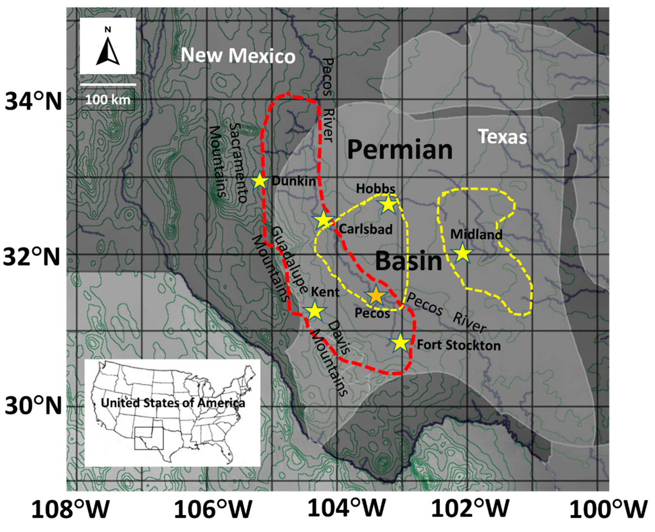
| Station Name | Network | Elevation (m) | Latitude °N/Longitude °W |
|---|---|---|---|
| Fort Stockton | TEXAS ASOS | 917 | 30.91194/102.91667 |
| Kent 9E | TEXAS DCP | 1221 | 31.08859/104.05490 |
| Midland Intl | TEXAS ASOS | 869 | 31.94662/102.20745 |
| Carlsbad | NM ASOS | 1004 | 32.33747/104.26328 |
| Dunken Raws | NM DCP | 1647 | 32.82560/105.18060 |
| Hobbs/Lea Co. | NM ASOS | 1115 | 32.68753/103.21703 |
2. Materials and Methods
2.1. TROPOMI Sensor Data and the Google Earth Engine (GEE)
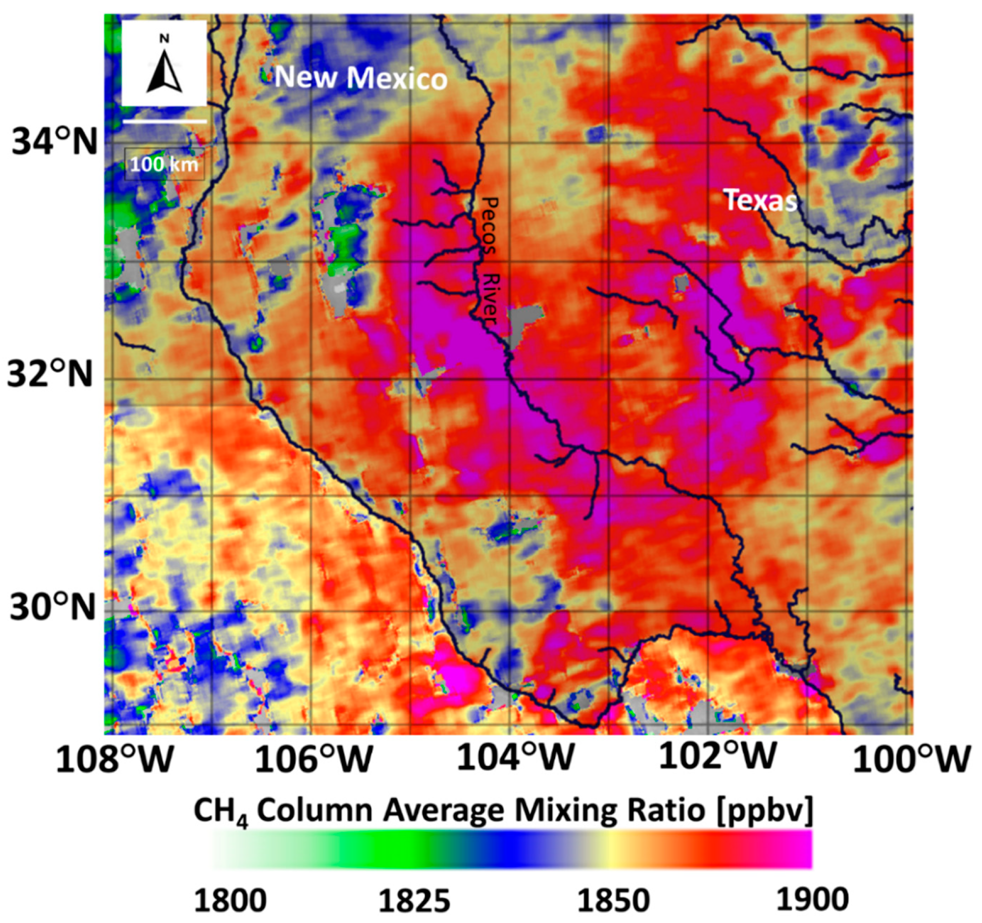
2.1.1. TROPOMI CH4 Data
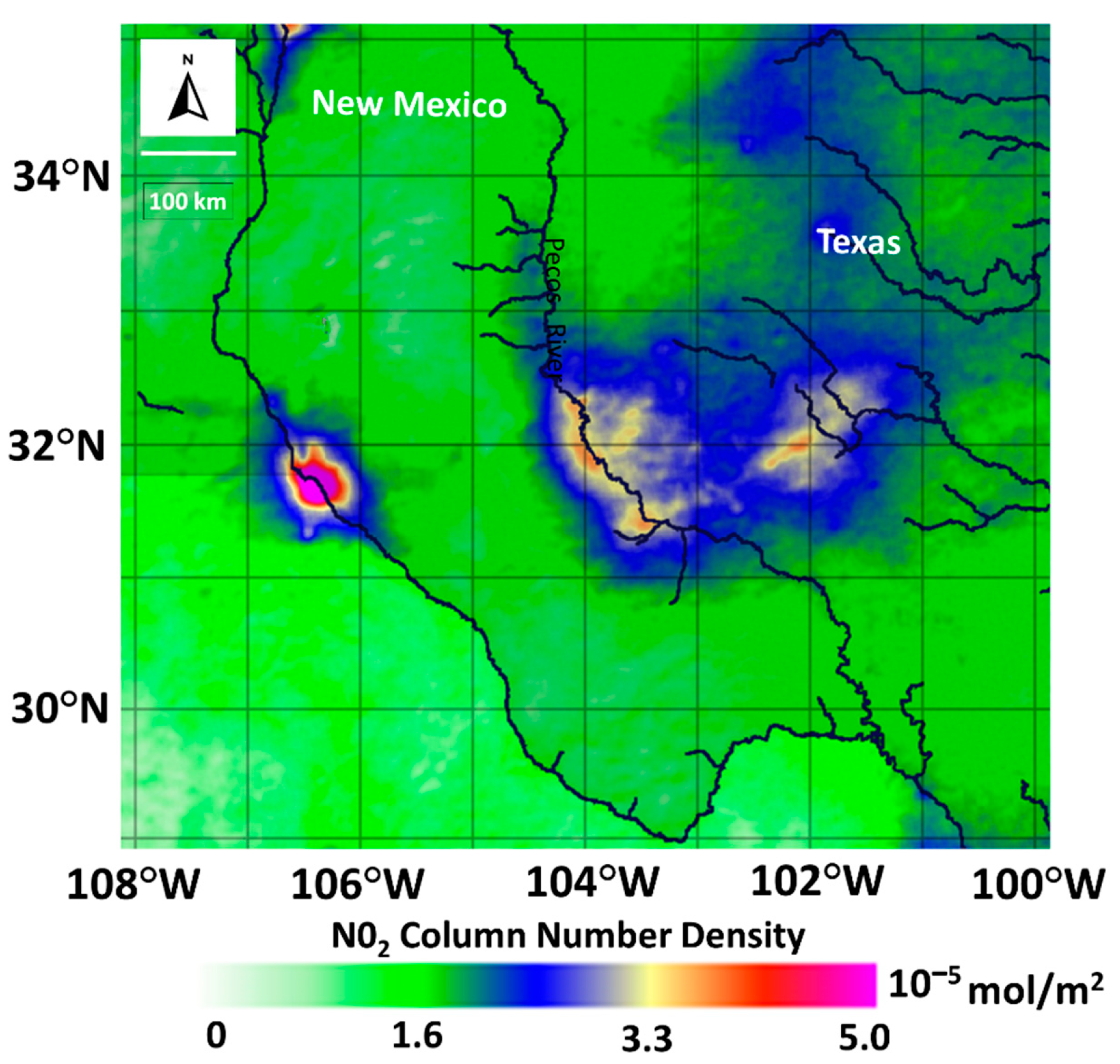
2.1.2. TROPOMI NO2 Data
2.2. Sources of Error
2.3. Meteorological 10-m Wind Observations and Analysis
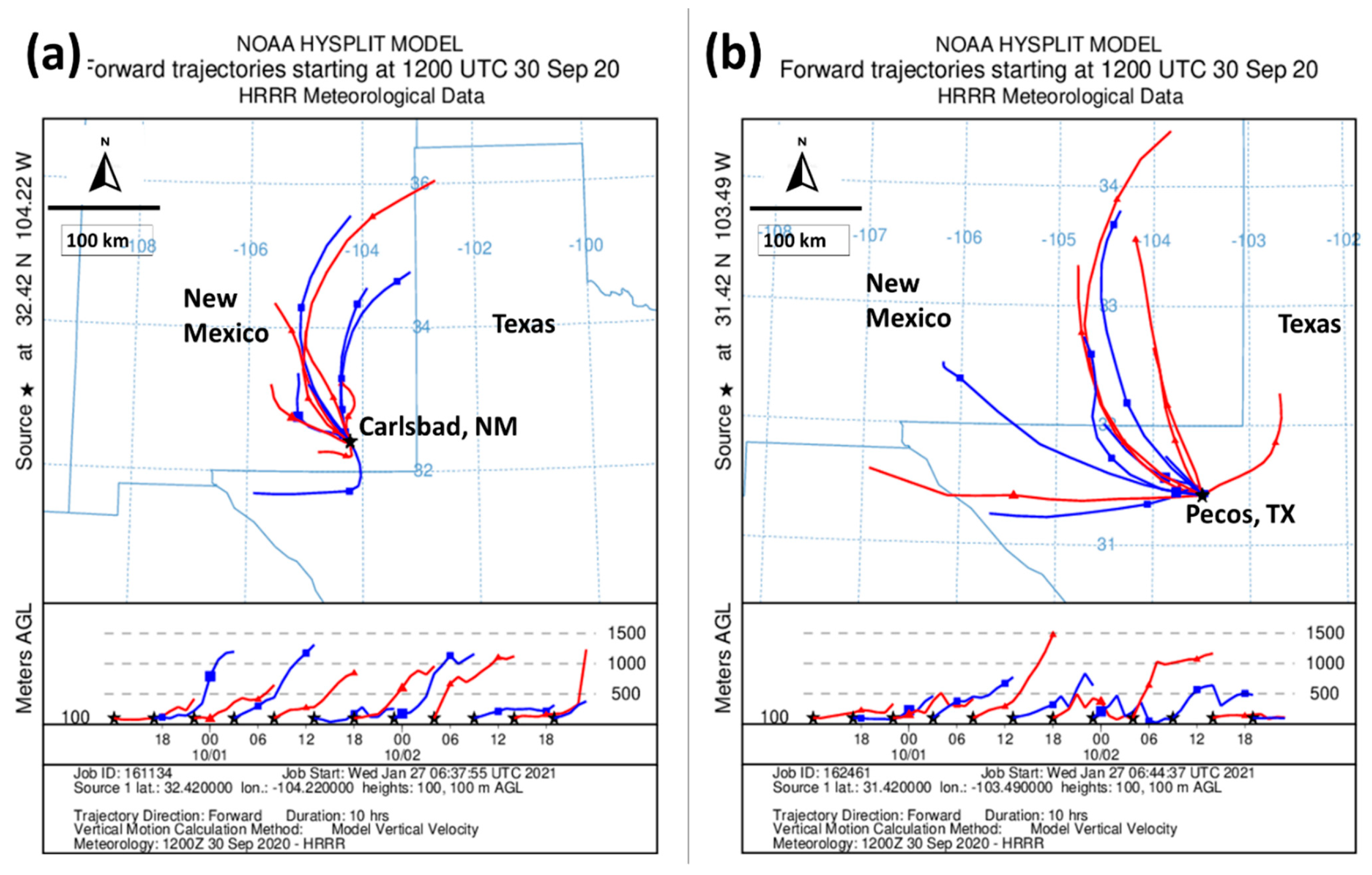
2.4. NCEP/NCAR Reanalyses and NOAA HYSPLIT Model
3. Results
3.1. TROPOMI Mean CH4 and NO2 1 December 2018–1 December 2020
3.2. Case Studies: Meteorological Drivers of Spatial and Temporal Variability of CH4 and NO2
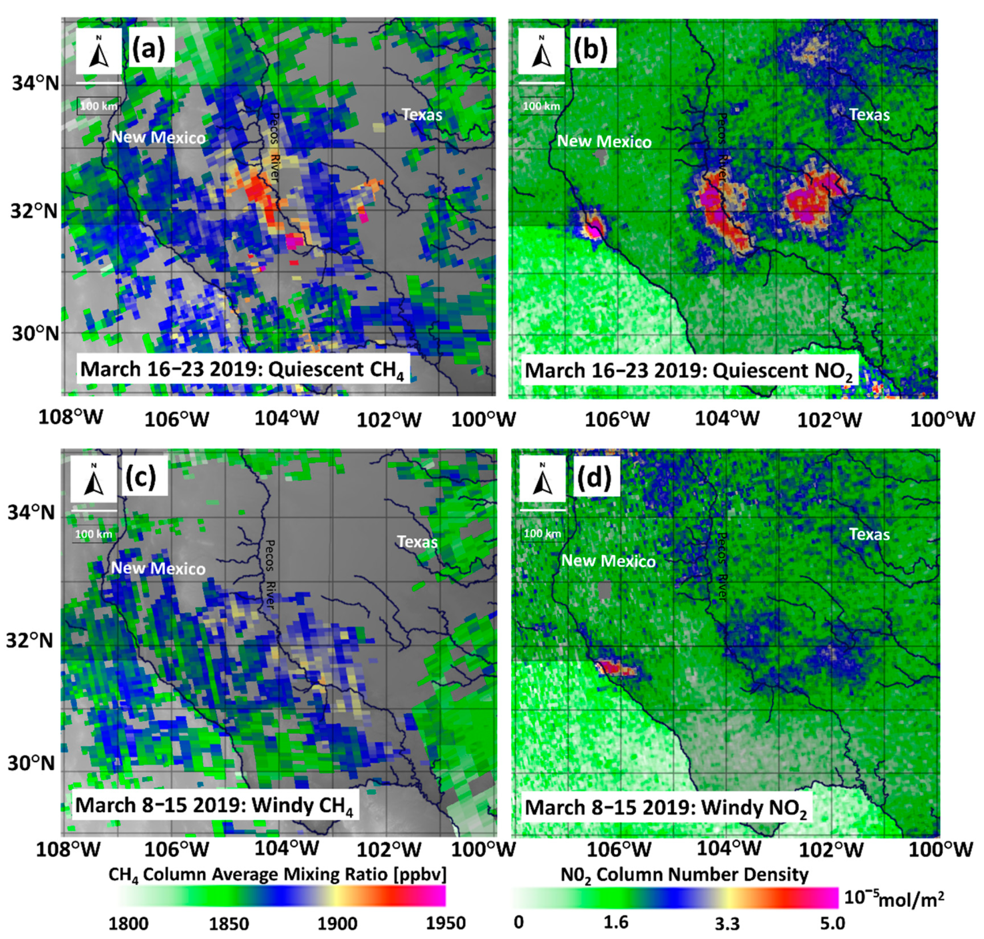
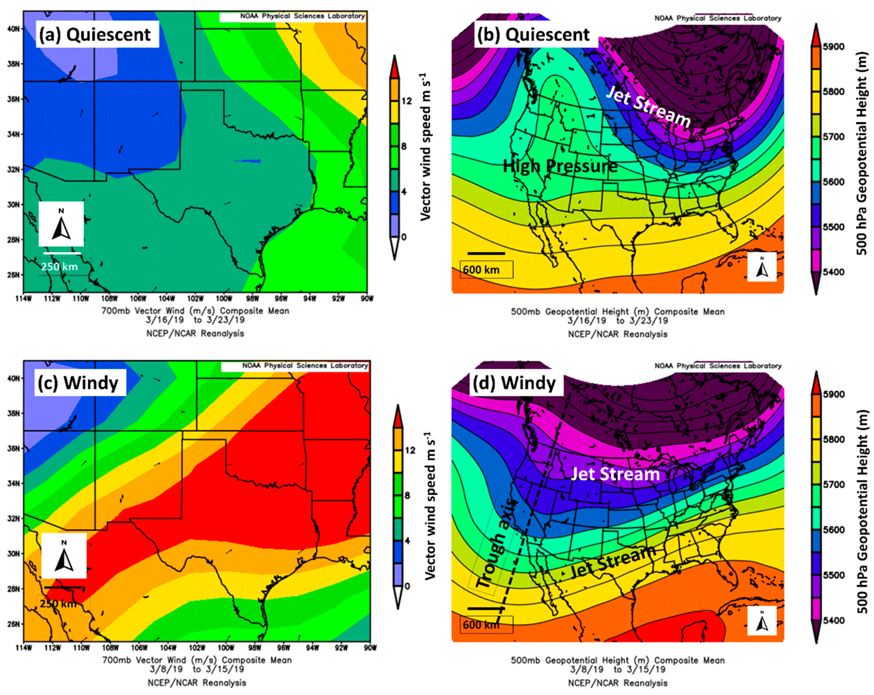
3.2.1. Short-Duration Meteorological Forcing Case Studies (8 Days)
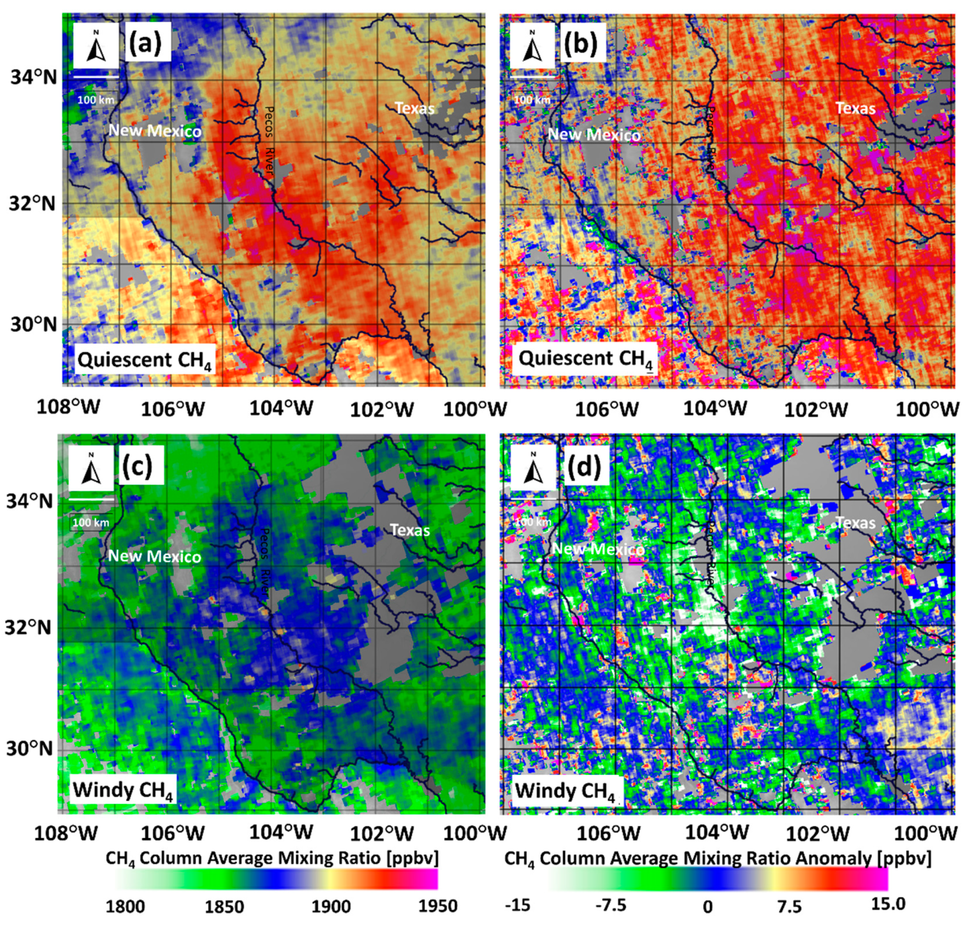
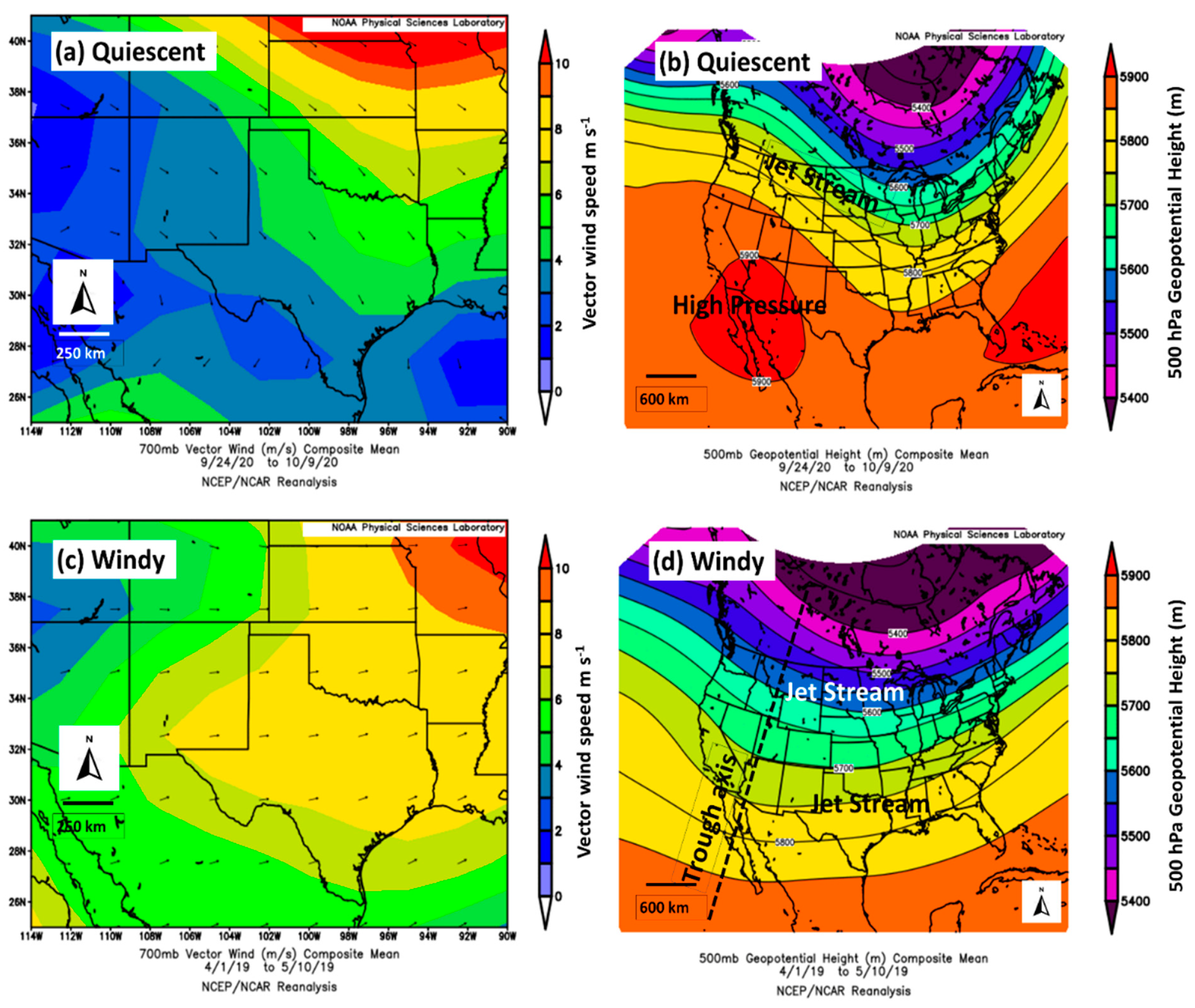
3.2.2. Longer-Term Meteorological Forcing Case Studies
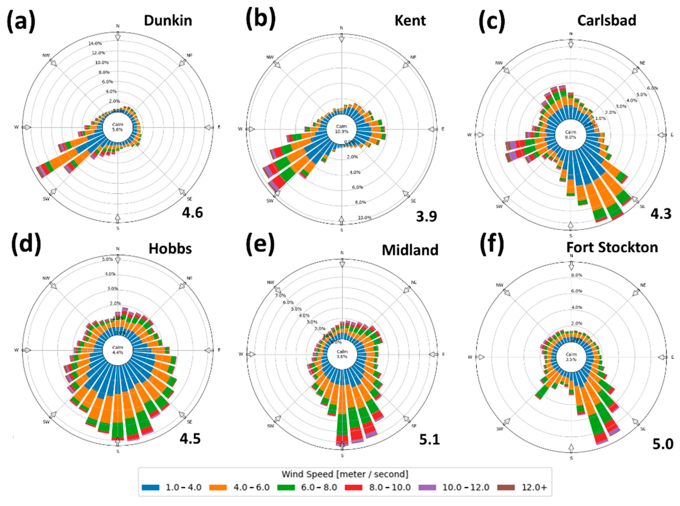
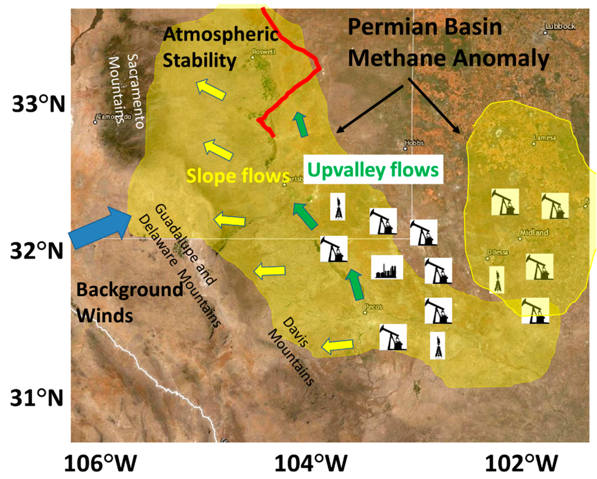
3.3. Surface Wind Climatology and Hypotheses for Western Basin CH4 Enhancement
4. Discussion
5. Conclusions
Supplementary Materials
Funding
Institutional Review Board Statement
Informed Consent Statement
Data Availability Statement
Acknowledgments
Conflicts of Interest
References
- Yazdan, M.M.S.; Ahad, M.T.; Jahan, I.; Mazumder, M. Review on the Evaluation of the Impacts of Wastewater Disposal in Hydraulic Fracturing Industry in the United States. Technologies 2020, 8, 67. [Google Scholar] [CrossRef]
- Kelly, E.N.; Schindler, D.W.; Hodson, P.V.; Short, J.W.; Radmanovich, R.; Nielsen, C.C. Oil sands development contributes elements toxic at low concentrations to the Athabasca River and its tributaries. Proc. Natl. Acad. Sci. USA 2010, 107, 16178–16183. [Google Scholar] [CrossRef]
- Nelson, R.; Heo, J. Monitoring environmental parameters with oil and gas developments in the Permian Basin, USA. Int. J. Environ. Res. Public Health 2020, 17, 4026. [Google Scholar] [CrossRef]
- Bruhwiler, L.M.; Basu, S.; Bergamaschi, P.; Bousquet, P.; Dlugokencky, E.; Houweling, S.; Ishizawa, M.; Kim, H.-S.; Locatelli, R.; Maksyutov, S.; et al. US CH4 emissions from oil and gas production: Have recent large increases been detected? J. Geophys. Res.-Atmos. 2017, 122, 4070–4083. [Google Scholar] [CrossRef]
- Thompson, R.L.; Nisbet, E.G.; Pisso, I.; Stohl, A.; Blake, D.; Dlugokencky, E.J.; Helmig, D.; White, J.W.C. Variability in atmospheric methane from fossil fuel and microbial sources over the last three decades. Geophys. Res. Lett. 2018, 45, 11499–11508. [Google Scholar] [CrossRef]
- Alvarez, R.A.; Zavala-Araiza, D.; Lyon, D.R.; Allen, D.T.; Barkley, Z.R.; Brandt, A.R.; Davis, K.J.; Herndon, S.C.; Jacob, D.J.; Karion, A.; et al. Assessment of methane emissions from the U.S. oil and gas supply chain. Science 2018, 361, 186–188. [Google Scholar] [CrossRef]
- Garcia-Gonzales, D.; Shonkoff, S.; Hays, J.; Jerrett, M. Hazardous air pollutants associated with upstream oil and natural gas development: A critical synthesis of current peer-reviewed literature. Annu. Rev. Public Health 2019, 40, 283–304. [Google Scholar] [CrossRef]
- Turner, A.J.; Frankenberg, C.; Kort, E.A. Interpreting contemporary trends in atmospheric methane. Proc. Natl. Acad. Sci. USA 2019, 116, 2805–2813. [Google Scholar] [CrossRef] [PubMed]
- Kaplan, G.; Avdan, Z.Y.; Avdan, U. Spaceborne Nitrogen Dioxide Observations from the Sentinel-5P TROPOMI over Turkey. Proceedings 2019, 18, 4. [Google Scholar] [CrossRef]
- Olstrup, H.; Johansson, C.; Forsberg, B.; Åström, C. Association between Mortality and Short-Term Exposure to Particles, Ozone and Nitrogen Dioxide in Stockholm, Sweden. Int. J. Environ. Res. Public Health 2019, 16, 1028. [Google Scholar] [CrossRef]
- Howarth, R.W. A bridge to nowhere: Methane emissions and the greenhouse gas footprint of natural gas. Energy Sci. Eng. 2014, 2, 47–60. [Google Scholar] [CrossRef]
- Grubert, E.A.; Brandt, A.R. Three considerations for modeling natural gas system methane emissions in the life cycle assessment. J. Clean. Prod. 2019, 222, 760–767. [Google Scholar] [CrossRef]
- Schwietzke, S.; Pétron, G.; Conley, S.; Pickering, C.; Mielke-Maday, I.; Dlugokencky, E.J.; Tans, P.P.; Vaughn, T.; Bell, C.; Zimmerle, D.; et al. Improved Mechanistic Understanding of Natural Gas Methane Emissions from Spatially Resolved Aircraft Measurements. Environ. Sci. Technol. 2017, 51, 7286–7294. [Google Scholar] [CrossRef]
- Foster, C.S.; Crosman, E.T.; Holland, L.; Mallia, D.V.; Fasoli, B.; Bares, R.; Horel, J.; Lin, J.C. Confirmation of elevated methane emissions in Utah’s Uintah Basin with ground-based observations and a high-resolution transport model. J. Geophys. Res.–Atmos. 2017, 15, 411–419. [Google Scholar] [CrossRef]
- Robertson, A.M.; Edie, R.; Field, R.A.; Lyon, D.; McVay, R.; Omara, M.; Zavala-Araiza, D.; Murphy, S.M. New Mexico Permian Basin measured well pad methane emissions are a factor of 5–9 times higher than U.S. EPA estimates. Environ. Sci. Technol. 2020, 54, 13926–13934. [Google Scholar] [CrossRef]
- Barkley, Z.R.; Lauvaux, T.; Davis, K.J.; Deng, A.; Miles, N.L.; Richardson, S.J.; Cao, Y.; Sweeney, C.; Karion, A.; Smith, M.; et al. Quantifying methane emissions from natural gas production in north-eastern Pennsylvania. Atmos. Chem. Phys. 2017, 17, 13941–13966. [Google Scholar] [CrossRef]
- Karion, A.; Sweeney, C.; Pétron, G.; Frost, G.; Hardesty, R.M.; Kofler, J.; Miller, B.R.; Newberger, T.; Wolter, S.; Banta, R.M.; et al. Methane emissions estimate from airborne measurements over a western United States natural gas field. Geophys. Res. Lett. 2013, 40, 4393–4397. [Google Scholar] [CrossRef]
- Cardoso-Saldana, F.J.; Allen, D.T. Projecting the Temporal Evolution of Methane Emissions from Oil and Gas Production Sites. Environ. Sci. Technol. 2020, 54, 14172–14181. [Google Scholar] [CrossRef] [PubMed]
- Lyon, D.R.; Hmiel, B.; Gautam, R.; Omara, M.; Roberts, K.; Barkley, Z.R.; David, K.J.; Miles, N.L.; Monteiro, V.C.; Richardson, S.J.; et al. Concurrent variation in oil and gas methane emissions and oil price during the COVID-19 pandemic. Atmos. Chem. Phys. Discuss. 2020. [Google Scholar] [CrossRef]
- Martin, R.V. Satellite remote sensing of air quuality. Atmos. Environ. 2008, 42, 7823–7843. [Google Scholar] [CrossRef]
- Schneising, O.; Burrows, J.P.; Dickerson, R.R.; Buchwitz, M.; Reuter, M.; Bovensmann, H. Remote sensing of fugitive methane emissions from oil and gas production in North American tight geologic formations. Earth’s Future 2014, 2, 548–558. [Google Scholar] [CrossRef]
- Kort, E.A.; Frankenberg, C.; Costigan, K.R.; Lindenmaier, R.; Dubey, M.K.; Wunch, D. Four corners: The largest US methane anomaly viewed from space. Geophys. Res. Lett. 2014, 41, GL061503. [Google Scholar] [CrossRef]
- Veefkind, J.; Aben, I.; McMullan, K.; Förster, H.; de Vries, J.; Otter, G.; Claas, J.; Eskes, H.; de Haan, J.; Kleipool, Q.; et al. TROPOMI on the ESA Sentinel-5 Precursor: A GMES mission for global observations of the atmospheric composition for climate, air quality and ozone layer applications. Remote Sens. Environ. 2012, 120, 7083. [Google Scholar] [CrossRef]
- Schneising, O.; Buchwitz, M.; Reuter, M.; Vanselow, S.; Bovensmann, H.; Burrows, J.P. Remote sensing of methane leakage from natural gas and petroleum systems revisited. Atmos. Chem. Phys. 2020, 20, 9169–9182. [Google Scholar] [CrossRef]
- De Gouw, J.A.; Veefkind, J.P.; Roosenbrand, E.; Dix, B.; Lin, J.C.; Landgraf, J.; Levelt, P.F. Daily satellite observations of methane from oil and gas production regions in the United States. Sci. Rep. 2020, 10, 1379. [Google Scholar] [CrossRef] [PubMed]
- Cersosimo, A.; Serio, C.; Masiello, G. TROPOMI NO2 Tropospheric Column Data: Regridding to 1 km Grid-Resolution and Assessment of their Consistency with In Situ Surface Observations. Remote Sens. 2020, 12, 2212. [Google Scholar] [CrossRef]
- Goldberg, D.L.; Lu, Z.; Streets, D.G.; de Foy, B.; Griffin, D.; McLinden, C.A.; Lamsal, L.N.; Krotkov, N.A.; Eskes, H. Enhanced capabilities of TROPOMI NO2: Estimating NOx from North American cities and power plants. Environ Sci Technol. 2019, 53, 12594–12601. [Google Scholar] [CrossRef]
- Vîrghileanu, M.; Săvulescu, I.; Mihai, B.-A.; Nistor, C.; Dobre, R. Nitrogen Dioxide (NO2) Pollution monitoring with Sentinel-5P satellite imagery over Europe during the coronavirus pandemic outbreak. Remote Sens. 2020, 12, 3575. [Google Scholar] [CrossRef]
- Fan, C.; Li, Y.; Guang, J.; Li, Z.; Elnashar, A.; Allam, M.; de Leeuw, G. The impact of the control measures during the COVID-19 outbreak on air pollution in China. Remote Sens. 2020, 12, 1613. [Google Scholar] [CrossRef]
- Griffin, D.; McLinden, C.A.; Racine, J.; Moran, M.D.; Fioletov, V.; Pavlovic, R.; Mashayekhi, R.; Zhao, X.; Eskes, H. Assessing the impact of corona-virus-19 on nitrogen dioxide levels over Southern Ontario, Canada. Remote Sens. 2020, 12, 4112. [Google Scholar] [CrossRef]
- Bauwens, M.; Compernolle, S.; Stavrakou, T.; Müller, J.-F.; van Gent, J.; Eskes, H.; Levelt, P.F.; van der, A.R.; Veefkind, J.P.; Vlietinck, J.; et al. Impact of coronavirus outbreak on NO2 pollution assessed using TROPOMI and OMI observations. Geophys. Res. Lett. 2020, 47. [Google Scholar] [CrossRef]
- Lorente, A.; Boersma, K.F.; Eskes, H.J.; Veefkind, J.P.; Van Geffen, J.H.G.M.; De Zeeuw, M.B.; Van Der Gon, H.A.C.D.; Beirle, S.; Krol, M.C. Quantification of nitrogen oxides emissions from build-up of pollution over Paris with TROPOMI. Sci. Rep. 2019, 9, 20033. [Google Scholar] [CrossRef]
- Solberg, S.; Walker, S.-E.; Schneider, P.; Guerreiro, C. Quantifying the Impact of the Covid-19 Lockdown Measures on Nitrogen Dioxide Levels throughout Europe. Atmosphere 2021, 12, 131. [Google Scholar] [CrossRef]
- Zhao, X.; Griffin, D.; Fioletov, V.; McLinden, C.; Cede, A.; Tiefengraber, M.; Müller, M.; Bognar, K.; Strong, K.; Boersma, F.; et al. Assessment of the quality of TROPOMI high-spatial-resolution NO2 data products in the Greater Toronto Area. Atmos. Meas. Tech. 2020, 13, 2131–2159. [Google Scholar] [CrossRef]
- Goldberg, D.L.; Anenberg, S.C.; Griffin, D.; McLinden, C.A.; Lu, Z.; Streets, D.G. Disentangling the impact of the COVID-19 lockdowns on urban NO2 from natural variability. Geophys. Res. Lett. 2020, 47. [Google Scholar] [CrossRef] [PubMed]
- Wang, Z.; Uno, I.; Yumimoto, K.; Itahashi, S.; Chen, X.; Yang, W.; Wang, Z. Impacts of COVID-19 lockdown, spring festival and meteorology on the NO2 variations in early 2020 over China based on in-situ observations, satellite retrievals and model simulations. Atmos. Environ. 2021, 244, 117972. [Google Scholar] [CrossRef] [PubMed]
- Griffin, D.; Zhao, X.; McLinden, C.A.; Boersma, F.; Bourassa, A.; Dammers, E.; Degenstein, D.; Eskes, H.; Fehr, L.; Fioletov, V.; et al. High-resolution mapping of nitrogen dioxide wWith TROPOMI: First results and validation over the Canadian oil sands. Geophys. Res. Lett. 2019, 46, 1049–1060. [Google Scholar] [CrossRef]
- Cunnold, D.M.; Steele, L.P.; Fraser, P.J.; Simmonds, P.G.; Prinn, R.G.; Weiss, R.F.; Porter, L.W.; O’Doherty, S.; Langenfelds, R.L.; Krummel, P.B.; et al. In situ measurements of atmospheric methane at GAGE/AGAGE sites during 1985–2000 and resulting source inferences. J. Geophys. Res. 2002, 107, 4225. [Google Scholar] [CrossRef]
- Hsu, Y.-K.; VanCuren, T.; Park, S.; Jakober, C.; Herner, J.; FitzGibbon, M.; Blake, D.R.; Parrish, D.D. Methane emissions inventory verification in southern California. Atmos. Environ. 2010, 44, 1–7. [Google Scholar] [CrossRef]
- Verhoelst, T.; Compernolle, S.; Pinardi, G.; Lambert, J.-C.; Eskes, H.J.; Eichmann, K.-U.; Fjæraa, A.M.; Granville, J.; Niemeijer, S.; Cede, A.; et al. Ground-based validation of the Copernicus Sentinel-5P TROPOMI NO2 measurements with the NDACC ZSL-DOAS, MAX-DOAS and Pandonia global networks. Atmos. Meas. Tech. 2021, 14, 481–510. [Google Scholar] [CrossRef]
- Dimitropoulou, E.; Hendrick, F.; Pinardi, G.; Friedrich, M.M.; Merlaud, A.; Tack, F.; De Longueville, H.; Fayt, C.; Hermans, C.; Laffineur, Q.; et al. Validation of TROPOMI tropospheric NO2 columns using dual-scan multi-axis differential optical absorption spectroscopy (MAX-DOAS) measurements in Uccle, Brussels. Atmos. Meas. Tech. 2020, 13, 5165–5191. [Google Scholar] [CrossRef]
- Judd, L.M.; Al-Saadi, J.A.; Szykman, J.J.; Valin, L.C.; Janz, S.J.; Kowalewski, M.G.; Eskes, H.J.; Veefkind, J.P.; Cede, A.; Mueller, M.; et al. Evaluating Sentinel-5P TROPOMI tropospheric NO2 column densities with airborne and Pandora spectrometers near New York City and Long Island Sound. Atmos. Meas. Tech. 2020, 13, 6113–6140. [Google Scholar] [CrossRef]
- Ialongo, I.; Virta, H.; Eskes, H.; Hovila, J.; Douros, J. Comparison of TROPOMI/Sentinel-5 Precursor NO2 observations with ground-based measurements in Helsinki. Atmos. Meas. Tech. 2020, 13, 205–218. [Google Scholar] [CrossRef]
- Wang, C.; Wang, T.; Wang, P.; Rakitin, V. Comparison and validation of TROPOMI and OMI NO2 observations over China. Atmosphere 2020, 11, 636. [Google Scholar] [CrossRef]
- Cheng, L.; Tao, J.; Valks, P.; Yu, C.; Liu, S.; Wang, Y.; Xiong, X.; Wang, Z.; Chen, L. NO2 retrieval from the environmental trace gases monitoring instrument (EMI): Preliminary results and intercomparison with OMI and TROPOMI. Remote Sens. 2019, 11, 3017. [Google Scholar] [CrossRef]
- Lorente, A.; Borsdorff, T.; Butz, A.; Hasekamp, O.; de Brugh, J.A.; Schneider, A.; Hase, F.; Kivi, R.; Wunch, D.; Pollard, D.F.; et al. Methane retrieved from TROPOMI: Improvement of the data product and validation of the first two years of measurements. Atmos. Meas. Tech. 2021, 14, 665–684. [Google Scholar] [CrossRef]
- Hasekamp, O.; Lorente, A.; Hu, H.; Butz, A.; de Brugh, A.A.; Landgraf, J. Algorithm theoretical baseline document for Sentinel-5 Precursor methane retrieval. Available online: https://sentinel.esa.int/documents/247904/2476257/Sentinel-5P-TROPOMI-ATBD-Methane-retrieval (accessed on 26 February 2021).
- Yang, Y.; Zhou, M.; Langerock, B.; Sha, M.K.; Hermans, C.; Wang, T.; Ji, D.; Vigouroux, C.; Kumps, N.; Wang, G.; et al. New ground-based Fourier-transform near-infrared solar absorption measurements of XCO2, XCH4 and XCO at Xianghe, China. Earth Syst. Sci. Data 2020, 12, 1679–1696. [Google Scholar]
- Schneising, O.; Buchwitz, M.; Reuter, M.; Bovensmann, H.; Burrows, J.P.; Borsdorff, T.; Deutscher, N.M.; Feist, D.G.; Griffith, D.W.T.; Hase, F.; et al. A scientific algorithm to simultaneously retrieve carbon monoxide and methane from TROPOMI onboard Sentinel-5 Precursor. Atmos. Meas. Tech. 2019, 12, 6771–6802. [Google Scholar] [CrossRef]
- Zhang, Y.; Gautam, R.; Pandey, S.; Omara, M.; Maasakkers, J.D.; Sadavarte, P.; Lyon, D.; Nesser, H.; Sulprizio, M.P.; Varon, D.J.; et al. Quantifying methane emissions from the largest oil-producing basin in the United States from space. Sci. Adv. 2020, 6, eaaz5120. [Google Scholar] [CrossRef]
- Tropomi Level 2 Products. Available online: www.tropomi.eu/data-products/level-2-products (accessed on 28 January 2021).
- Van Geffen, J.H.G.M.; Eskes, H.J.; Boersma, K.F.; Maasakkers, J.D.; Veefkind, J.P. TROPOMI ATBD of the Total and Tropospheric NO2 Data Products. Available online: http://www.tropomi.eu/documents/atbd/ (accessed on 10 December 2020).
- Gorelick, N.; Hancher, M.; Dixon, M.; Ilyushchenko, S.; Thau, D.; Moore, R. Google Earth Engine: Planetary-scale geospatial analysis for everyone. Remote Sens. Environ. 2017, 202, 18–27. [Google Scholar] [CrossRef]
- Tamiminia, H.; Salehi, B.; Mahdianpari, M.; Quackenbush, L.; Adeli, S.; Brisco, B. Google Earth Engine for geo-big data applications: A meta-analysis and systematic review. ISPRS J. Photogramm. Remote Sens. 2020, 164, 152–170. [Google Scholar] [CrossRef]
- Topical Collection Special Issue of Remote Sensing: “Google Earth Engine Applications”. Available online: https://www.mdpi.com/journal/remotesensing/special_issues/GEE (accessed on 20 December 2020).
- Sentinel-5P OFFL CH4. Available online: https://developers.google.com/earth-engine/datasets/catalog/COPERNICUS_S5P_OFFL_L3_CH4 (accessed on 19 December 2020).
- Harpconvert. Available online: http://stcorp.github.io/harp/doc/html/harpconvert.html (accessed on 13 February 2021).
- Sentinel-5P OFFL NO2. Available online: https://developers.google.com/earth-engine/datasets/catalog/COPERNICUS_S5P_OFFL_L3_NO2 (accessed on 15 December 2020).
- Hu, H.; Hasekamp, O.; Butz, A.; Galli, A.; Landgraf, J.; de Brugh, J.A.; Borsdorff, T.; Scheepmaker, R.; Aben, I. The operational methane retrieval algorithm for TROPOMI. Atmos. Meas. Tech. 2016, 9, 5423–5440. [Google Scholar] [CrossRef]
- Van Geffen, J.; Boersma, K.F.; Eskes, H.; Sneep, M.; Linden, M.T.; Zara, M.; Veefkind, J.P. S5P TROPOMI NO2 slant column retrieval: Method, stability, uncertainties and comparisons with OMI. Atmos. Meas. Tech. 2020, 13, 1315–1335. [Google Scholar] [CrossRef]
- Horel, J.; Splitt, M.; Dunn, L.; Pechmann, J.; White, B.; Ciliberti, C.; Lazarus, S.; Slemmer, J.; Zaff, D.; Burks, J. Mesowest: Cooperature Mesonets in the Western United States. Bull. Am. Meteorol. Soc. 2002, 83, 211–226. [Google Scholar] [CrossRef]
- Mesowest. Available online: https://mesowest.utah.edu/ (accessed on 19 December 2020).
- Iowa State Mesonet. Available online: https://mesonet.agron.iastate.edu/ (accessed on 28 January 2020).
- NCEP/NCAR Reanalysis Composites. Available online: https://www.psl.noaa.gov/data/composites/hour/ (accessed on 30 January 2021).
- Draxler, R.R.; Rolph. HYSPLIT (Hybrid Single-Particle Lagrangian Integrated Trajectory) model access via NOAA ARL READY Website. Available online: http://www.arl.noaa.gov/ready/hysplit4.html (accessed on 28 January 2021).
- Stein, A.F.; Draxler, R.R.; Rolph, G.D.; Stunder, B.J.B.; Cohen, M.D.; Ngan, F. NOAA’s HYSPLIT Atmospheric Transport and Dispersion Modeling System. Bull. Am. Meteorol. Soc. 2015, 96, 2059–2077. [Google Scholar] [CrossRef]
- Benjamin, S.G.; Weygandt, S.S.; Brown, J.M.; Hu, M.; Alexander, C.R.; Smirnova, T.G.; Olson, J.B.; James, E.P.; Dowell, D.C.; Grell, G.A.; et al. A North American hourly assimilation and model forecast cycle: The rapid refresh. Mon. Weather Rev. 2016, 144, 1669–1694. [Google Scholar] [CrossRef]
- He, T.; Gao, F.; Liang, S.; Peng, Y. Mapping Climatological Bare Soil Albedos over the Contiguous United States Using MODIS Data. Remote Sens. 2019, 11, 666. [Google Scholar] [CrossRef]
- Foster, C.S.; Crosman, E.T.; Horel, J.D.; Lyman, S.N.; Fasoli, B.; Bares, R.; Lin, J.C. Quantifying methane emissions in the Uintah Basin during wintertime stagnation episodes. Elem. Sci. Anthr. 2019, 7, 24. [Google Scholar] [CrossRef]
- Benedict, K.B.; Prenni, A.J.; El-Sayed, M.M.H.; Hecobian, A.; Zhou, Y.; Gebhart, K.A.; Sive, B.C.; Schichtel, B.A.; Collett, J.L. Volatile organic compounds and ozone at four national parks in the southwestern United States. Atmos. Environ. 2020, 239, 117783. [Google Scholar] [CrossRef]
- De Wekker, S.F.J.; Kossmann, M.; Knievel, J.C.; Giovannini, L.; Gutmann, E.D.; Zardi, D. Meteorological Applications Benefiting from an Improved Understanding of Atmospheric Exchange Processes over Mountains. Atmosphere 2018, 9, 371. [Google Scholar] [CrossRef]
- Miao, Y.; Liu, S.; Sheng, L.; Huang, S.; Li, J. Influence of Boundary Layer Structure and Low-Level Jet on PM2.5 Pollution in Beijing: A Case Study. Int. J. Environ. Res. Public Health 2019, 16, 616. [Google Scholar] [CrossRef] [PubMed]
- Evans, J.M.; Helmig, D. Investigation of the influence of transport from oil and natural gas regions on elevated ozone levels in the northern Colorado front range. J. Air Waste Manag. Assoc. 2017, 67, 196–211. [Google Scholar] [CrossRef] [PubMed]
- Janardanan, R.; Maksyutov, S.; Tsuruta, A.; Wang, F.; Tiwari, Y.K.; Valsala, V.; Ito, A.; Yoshida, Y.; Kaiser, J.W.; Janssens-Maenhout, G.; et al. Country-Scale Analysis of Methane Emissions with a High-Resolution Inverse Model Using GOSAT and Surface Observations. Remote Sens. 2020, 12, 375. [Google Scholar] [CrossRef]
- Kuze, A.; Kikuchi, N.; Kataoka, F.; Suto, H.; Shiomi, K.; Kondo, Y. Detection of Methane Emission from a Local Source Using GOSAT Target Observations. Remote Sens. 2020, 12, 267. [Google Scholar] [CrossRef]
- Ayasse, A.K.; Dennison, P.E.; Foote, M.; Thorpe, A.K.; Joshi, S.; Green, R.O.; Duren, R.M.; Thompson, D.R.; Roberts, D.A. Methane Mapping with Future Satellite Imaging Spectrometers. Remote Sens. 2019, 11, 3054. [Google Scholar] [CrossRef]
- Tian, J.; Fang, C.; Qiu, J.; Wang, J. Analysis of Pollution Characteristics and Influencing Factors of Main Pollutants in the Atmosphere of Shenyang City. Atmosphere 2020, 11, 766. [Google Scholar] [CrossRef]
- He, J.; Lu, S.; Yu, Y.; Gong, S.; Zhao, S.; Zhou, C. Numerical Simulation Study of Winter Pollutant Transport Characteristics over Lanzhou City, Northwest China. Atmosphere 2018, 9, 382. [Google Scholar] [CrossRef]


| Resolution. | Product | Band Name (Units) |
|---|---|---|
| 0.01 arc degrees | GEE Sentinel-5P OFFL CH4 | Band name: CH4_column_volume_mixing_ratio_dry_air (ppbv) |
| 0.01 arc degrees | GEE Sentinel-5P OFFL NO2 | Band name: NO2_column_volume_number_density (mol/m2) |
Publisher’s Note: MDPI stays neutral with regard to jurisdictional claims in published maps and institutional affiliations. |
© 2021 by the author. Licensee MDPI, Basel, Switzerland. This article is an open access article distributed under the terms and conditions of the Creative Commons Attribution (CC BY) license (http://creativecommons.org/licenses/by/4.0/).
Share and Cite
Crosman, E. Meteorological Drivers of Permian Basin Methane Anomalies Derived from TROPOMI. Remote Sens. 2021, 13, 896. https://doi.org/10.3390/rs13050896
Crosman E. Meteorological Drivers of Permian Basin Methane Anomalies Derived from TROPOMI. Remote Sensing. 2021; 13(5):896. https://doi.org/10.3390/rs13050896
Chicago/Turabian StyleCrosman, Erik. 2021. "Meteorological Drivers of Permian Basin Methane Anomalies Derived from TROPOMI" Remote Sensing 13, no. 5: 896. https://doi.org/10.3390/rs13050896
APA StyleCrosman, E. (2021). Meteorological Drivers of Permian Basin Methane Anomalies Derived from TROPOMI. Remote Sensing, 13(5), 896. https://doi.org/10.3390/rs13050896