Evaluation of MODIS Aerosol Optical Depth and Surface Data Using an Ensemble Modeling Approach to Assess PM_2.5 Temporal and Spatial Distributions

Abstract

The use of statistical models and machine-learning techniques along satellite-derived aerosol optical depth (AOD) is a promising method to estimate ground-level particulate matter with an aerodynamic diameter of ≤2.5 μm (PM_2.5), mainly in urban areas with low air quality monitor density. Nevertheless, the relationship between AOD and ground-level PM_2.5 varies spatiotemporally and differences related to spatial domains, temporal schemes, and seasonal variations must be assessed. Here, an ensemble multiple linear regression (EMLR) model and an ensemble neural network (ENN) model were developed to estimate PM_2.5 levels in the Monterrey Metropolitan Area (MMA), the second largest urban center in Mexico. Four AOD-SDSs (Scientific Datasets) from MODIS Collection 6 were tested using three spatial domains and two temporal schemes. The best model performance was obtained using AOD at 0.55 µm from MODIS-Aqua at a spatial resolution of 3 km, along meteorological parameters and daily scheme. EMLR yielded a correlation coefficient (R) of ~0.57 and a root mean square error (RMSE) of ~7.00 μg m⁻³. ENN performed better than EMLR, with an R of ~0.78 and RMSE of ~5.43 μg m⁻³. Satellite-derived AOD in combination with meteorology data allowed for the estimation of PM_2.5 distributions in an urban area with low air quality monitor density.

1. Introduction

Particulate matter with an aerodynamic diameter of less than or equal to 2.5 μm (PM_2.5) is a critical indicator for measuring the air quality in a given area [1,2]. PM_2.5 concentrations are usually monitored using air quality measurement stations with spatial representativeness ranging from 500 m to 4 km in diameter for local, neighborhood scales [3]. However, in many regions of the world (e.g., Latin America), ground-level measurements of PM_2.5 are scarce or non-existent [4], making it difficult to determine the behavior and distribution of aerosols at local and regional scales. Satellite data are potentially useful for deriving indirect estimates of ground PM_2.5 pollution from aerosol optical properties, overcoming the well-known spatial limitation of traditional measurements. Such estimates may be regarded as a complementary cost effective method for PM_2.5 monitoring at local and regional scales in locations with non-existent or without extensive ground-based PM_2.5 monitoring networks [5,6].

Recently, Shin et al. (2019) [7] performed an extensive review of the use of satellite-derived aerosol products to predict ground-level PM, focusing on modeling techniques, sensor types, and geographic areas of study. Machine-learning techniques such as artificial neural networks (ANNs) have been explored and used to combine ground-level concentrations and satellite retrievals. However, most studies have aimed at the long-term forecasting of criteria pollutants using models that include meteorological variables and source emissions as predictors. Satellite AOD data have also been used along remotely sensed nighttime light (NTL) imagery to predict ground-level PM_2.5 at a regional scale in mixed -urban, suburban, and rural-areas [8], or random forest (RF) regression to reconstruct area-scale satellite missing AOD retrievals and the stochastic autoregressive integrated moving average (ARIMA) model to enhance AOD data coverage and improve the forecast of AOD profiles [9].

Despite many technological and computational advances, Shin et al. (2019) [7] identified the need to increase the spatial extension of PM monitoring to a global scale, the potential use of satellite-derived products and numerical model outputs (e.g., reanalysis models and photochemical models) to improve PM estimation accuracy and gap-filling, the necessity of more advanced modeling techniques (e.g., data assimilations and machine-learning) for pollution estimation and prediction, the need for improved emission data, and the possibility of performing short-term (hours to days) PM estimations.

One of the most robust aerosol parameters derived in satellite aerosol products is the aerosol optical depth (AOD) [10,11]. AOD is the integral of the aerosol extinction along a vertical atmospheric column from the Earth’s surface to the top of the atmosphere. It has been extensively used to estimate PM_2.5 concentrations (e.g., [10,11,12,13,14]. The AOD–PM_2.5 relationship, however, varies in space and time and needs to be specifically assessed for different regions and seasons [15]. Despite Latin America being one of the most urbanized, populated, and polluted regions in the world, where most cities lack robust ground-based PM_2.5 monitoring networks, few studies have examined the relationship between AOD and PM_2.5 in this region (e.g., [16,17,18,19,20]).

AOD can be obtained from different remote-sensing instruments, for example, the multiangle imaging spectroradiometer (MISR), the visible infrared imaging radiometer suite (VIIRS), and the moderate-resolution imaging spectroradiometer (MODIS) [21]. Nonetheless, the use of MODIS [22,23] presents advantages because of its twice daily measurements, high-resolution (1, 3, and 10 km at nadir), long-term records (since 2000 for Terra and 2002 for Aqua), and validation with other satellite products [24].

Different algorithms for retrieving AOD (e.g., dark target (DT) algorithms over land, the DT over-ocean (water) algorithm, and deep blue (DB) algorithms (over land)) have been developed and are included in the MODIS Atmosphere data product suite. All three have been refined in the “Collection 6” (C6) MODIS reprocessing. Moreover, a combined DT and DB dataset has also been added based on piecewise fixed thresholds using the normalized difference vegetation index (NDVI). Because distinctive assumptions have been made in the algorithm retrieval procedures, bestowing each with strengths and limitations that also influence the AOD–PM_2.5 relationship, it is crucial to evaluate MODIS aerosol products for specific regions and periods of time [25].

This study evaluates the performance of the DT and DB algorithms from MODIS C6 in the estimation of PM_2.5 concentrations over the Monterrey Metropolitan Area (MMA)—one of the major urban centers in northeastern Mexico with non-dominant land coverage—from 2010 to 2017. In this study, MODIS C6 products, using different retrieval algorithms, were tested for three spatial domains and two temporal schemes to ascertain which dataset best describes the relationship between AOD and PM_2.5 ground-based data. Backward and forward stepwise regressions were used to identify the meteorological variables that influence the AOD–PM_2.5 relationship, and ensemble multiple linear regression (EMLR) and ensemble neural network (ENN) models were developed and validated for the estimation of local PM_2.5 concentrations.

To the best of our knowledge, this is the first such study within this region; only Carmona et al. (2020) [17] have recently evaluated the ability of the Modern-Era Retrospective Analysis for Research and Application model, version 2 (MERRA-2), aerosol components to represent PM_2.5 ground concentrations. Therefore, this study contributes to the knowledge and understanding of the performance of MODIS AOD–PM_2.5 retrieval algorithms over urban, mixed-use land coverage areas with limited ground-based observations.

2. Materials and Methods

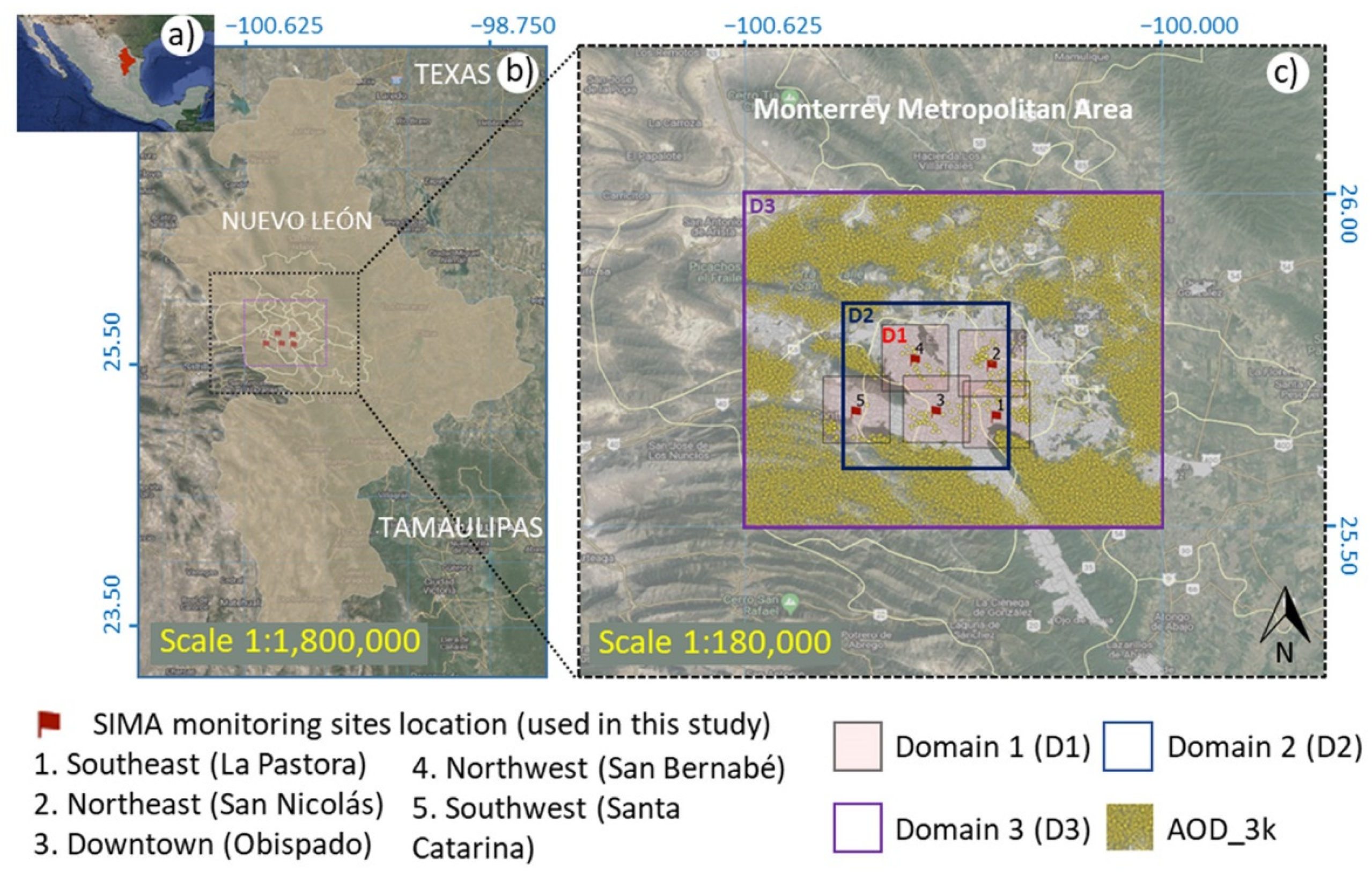
2.1. Study Area

This study was conducted within the MMA, Mexico, from January 2010 to December 2017. The MMA (25°40′N, 100°20′W) is located in the State of Nuevo León, in Northeast Mexico, approximately 720 km north of Mexico City and approximately 230 km south of the United States border. The MMA is composed of 18 municipalities (Figure 1) and has an area of 7657 km² [26]. It is the largest urban area in northeastern Mexico and the second most populous in the country with 5.7 million inhabitants [27]. The study area is located on the boundary of the province of Sierra Madre Oriental, which is characterized by mountainous relief with alternating mountain ranges and valleys [28]. Vertical drops of over 1400 m occur, with minimum and maximum elevations of 542 m and 1993 m above sea level, respectively. The lower altitude areas correspond to valleys, where the population of the MMA is settled [29].

The study area was analyzed using three spatial domains. Domain 1 (D1) contains ground data from each ground-level monitoring site versus AOD averaged at a resolution of 0.10° × 0.10° (collocated AOD values are contained in this domain); Domain 2 (D2) contains ground data (averaged from the five sites) versus AOD averaged at a resolution of 0.25° × 0.25°; and Domain 3 (D3) contains ground data (averaged from the five sites) versus AOD averaged at a resolution of 0.500° × 0.625°. Domains 1, 2, and 3 represent neighborhood, urban, and regional scales, respectively, as defined by EPA (2008) [3].

2.2. Ground-Based Air Quality Monitoring and PM_2.5 Pollution in the MMA

The MMA has a network of air quality monitoring stations known locally as the Sistema Integral de Monitoreo Ambiental (SIMA) composed currently of 13 monitoring sites. Criteria air pollutants (O₃, SO₂, NO_x [NO_x = NO + NO₂], CO, PM_2.5, and PM₁₀) and meteorological variables (temperature, relative humidity, wind speed, wind direction, pressure, precipitation, and solar radiation) are continuously monitored, with the data summarized as hourly averages.

The MMA currently has a status of nonattainment with respect to the Mexican Air Quality Standards for PM_2.5 [30,31]. In 2015, the MMA exhibited annual averages in the range of 20–34 μg m⁻³ for PM_2.5, exceeding the PM_2.5 national air quality standard of 12 μg m⁻³ [32]. For 50 days of 2019, the PM_2.5 concentrations exceeded the 24-h average limit of 45 μg m⁻³ set by the Mexican standard [33]. Seasonal variations in the PM_2.5 concentrations have also been observed, with winter showing the highest concentrations while the lowest concentrations were observed during summer and the first weeks of fall [34].

There are multiple sources of fine PM air pollution in the MMA. Source apportionment studies based on the chemical characterization of ambient air aerosols conducted in the MMA have found that approximately 64% of PM_2.5 comes from direct or precursor vehicle emissions [35,36,37]. Other significant sources include meat-cooking operations and biomass burning. Industrial activities, garbage burning, biogenic emissions, and resuspended dust also contribute to air pollution in the MMA [38].

2.3. Data

2.3.1. Ground-Based PM_2.5 and Meteorological Data

The PM_2.5 and meteorological data were retrieved for the period from 2010 to 2017 at five urban ambient air monitoring sites in the SIMA network (the Southeast, Northeast, Downtown, Northwest, and Southwest stations; Figure 1). These sites were chosen because they provided continuous valid PM_2.5 records during the study period. Specifically, the PM_2.5 instruments are based on the beta-ray attenuation method and continuous weighing with a microbalance, providing automatic and continuous measurements and concentration recordings. SIMA instrumentation records PM_2.5 every minute; the records are then validated and stored as 1-h averages. The Mexican standards NOM-035-SEMARNAT-1993 [39] and NOM-156-SEMARNAT-2012 [40] are followed to accomplish the calibration, maintenance procedures, and quality assurance/quality control protocols.

2.3.2. MODIS AOD Data

Four AOD scientific datasets (SDSs) from Aqua MODIS C6 aerosol products (MYD04_3K and MYD04_L2) were evaluated to identify which dataset best described the relationship between AOD and the ground-based data for the estimation of PM_2.5 in the MMA.

Table 1. Aerosol optical depth (AOD)-scientific datasets (SDSs) from the moderate-resolution imaging spectroradiometer (MODIS) aerosol products.

Product	SDS	Resolution
AOD_3K	Optical_Depth_Land_And_Ocean 1	3 km
AOD_DT	Optical_Depth_Land_And_Ocean 1	10 km
AOD_DB	Deep_Blue_Aerosol_Optical_Depth_550_Land_Best_Estimate 2	10 km
AOD_Cb	AOD_550_Dark_Target_Deep_Blue_Combined 3	10 km

¹ This SDS contains dark target AOD at 0.55 µm for land with a quality assurance (QA) = 3. ² This SDS contains deep blue AOD at 0.55 µm for land with QA = 2 and 3. ³ “AOD_550_Dark_Target_Deep_Blue_Combined_Algorithm_Flag” QA = 2 and 3.

lists the AOD-SDSs used in this study.

Both the Optical_Depth_Land_And_Ocean SDS from MYD04_L2 (AOD_DT) and from MYD04_3k (AOD_3K) at 10 km and 3 km at nadir, respectively, are MODIS products retrieved using the DT algorithm. The surface scheme used in the DT algorithm identifies dark target pixels (mainly vegetated areas). The DT algorithm identifies four distinct fine-dominated aerosol models: continental, moderately absorbing, strongly absorbing smoke, and weakly absorbing (urban/industrial) [41].

The DB AOD-SDS from MYD04_L2 (AOD_DB) is a MODIS product retrieved using the DB algorithm at 10 km at nadir. Three surface categories were derived from MODIS DB C6 including arid and semiarid regions, general vegetation, and urban/built-up and transitional regions. The DB algorithm performs aerosol retrieval for non-spherical and absorbing aerosols including (1) dust aerosols, (2) mixtures of dust/smoke aerosols, and (3) strongly absorbing dust [42].

Finally, the Cb AOD-SDS from the MYD04_L2 product (AOD_Cb) is a merged product reported at 10 km. This dataset was designed to provide a single dataset that combines the best of DB and DT into a data product with fewer gaps [43]. The merge procedure is based on NDVI criteria (NDVI > 0.30 = DT; NDVI < 0.20 = DB; 0.2 < NDVI < 0.30 = merge).

2.4. Model Development and Validation

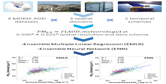
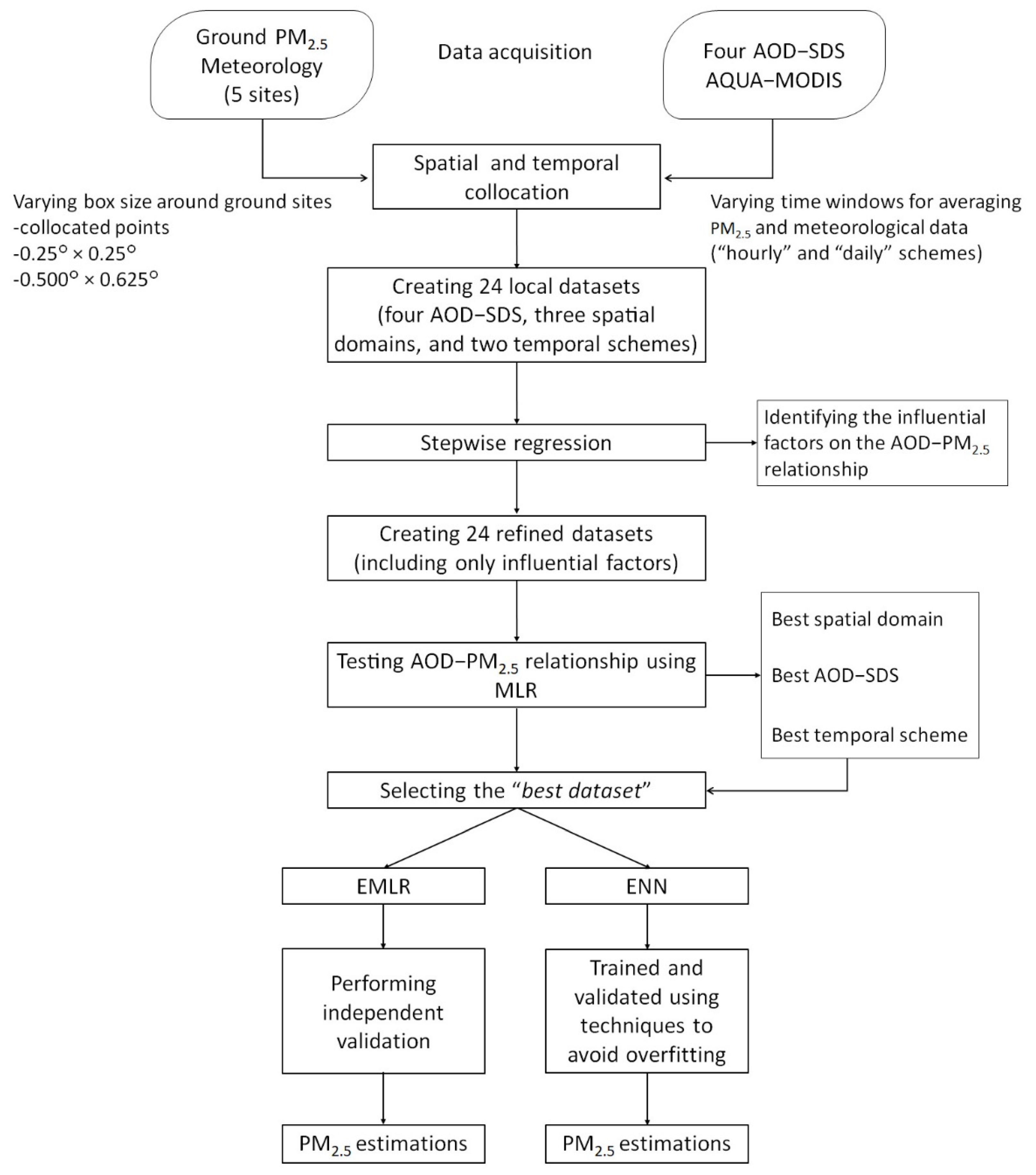
2.4.1. Data Processing Overview

Figure 2 provides an overview of the methodology followed in this study. The first step involved data acquisition, spatial and temporal collocation, and the testing of 24 MODIS datasets (four AOD-SDSs for three domains and two temporal schemes) using stepwise regression to determine the meteorological variables that influence the AOD–PM_2.5 relationship in the MMA. In the second step, the 24 refined datasets (which included only the influential meteorological variables in the AOD–PM_2.5 relationship) were analyzed using a multiple linear regression (MLR) model to identify which AOD-SDS, domain, and temporal schemes showed the best correlation in the MMA. The resulting dataset was labeled the “best dataset”. In the third step, an ensemble model based on MLR was developed to validate the robustness of the best dataset. Then, several neural networks (NNs) were trained and validated to build an ENN model to estimate the PM_2.5 concentrations.

2.4.2. PM_2.5 Concentration and MODIS AOD Spatiotemporal Collocation

The four MODIS AOD datasets and the ground-based data were geo-referenced to geographic latitude/longitude (WGS84) coordinates. To explore spatial differences in the AOD selection, the effect of the box size (the number of pixels in the spatial collocation) around the ground sites on the mean AOD was evaluated. The four AOD-SDSs were tested along with ground-based data using three spatial domains (Figure 1c) and two temporal averaging schemes (denoted “hourly” and “daily”) to identify sample AOD data to develop statistical models that best describe the relationship between PM_2.5, AOD, and the meteorology.

The hourly scheme recognizes that the Aqua satellite crosses the MMA at 13:30 local time (±55 min). Accordingly, ground-level PM_2.5 and meteorological values were processed by averaging the observations measured from 12:00 to 15:00 local time. This scheme tries to make connections with ground-level air masses similar to those observed by MODIS. In the daily scheme, data were processed by averaging the PM_2.5 and 1-h average meteorological observations reported from midnight to midnight, local time. This scheme is used to represent the PM_2.5 data according to the 24-h Mexican standard NOM-025-SSA1-2014 [33], which requires a threshold of 75% data capture (i.e., 18 hourly records) to consider the data as valid and representative for a given day. Missing days were excluded from our analysis. The average AOD at the satellite overpass time was used to represent the AOD mean values in both schemes, against which the ground-level average observations were contrasted.

2.4.3. MLR

Twenty-four different datasets (AOD from four MODIS SDSs, three spatial domains, and two temporal schemes) were analyzed to identify the best dataset, namely, the dataset that best described the relationship between the satellite-derived AOD and the ground-level meteorological observations with surface-level PM_2.5 in the MMA. The effect of the proposed spatiotemporal averaging schemes on this relationship was evaluated by assessing the MLR models.

To sequentially identify the best subset of independent variables to incorporate into the regression equation, all meteorological variables recorded by SIMA (temperature, relative humidity, wind speed, wind direction, rain, pressure, and solar radiation) along with the AOD data were included in the 24 datasets. The final datasets (refined datasets) were selected using a stepwise regression method to achieve the highest level of estimation accuracy possible, and only those meteorological variables that were statistically significant and most significantly correlated with the dependent variable (PM_2.5) were retained. Forward and backward stepwise regression procedures were applied, and a significance level (p-value) of 0.05 was used for the inclusion and exclusion of variables.

The refined datasets were tested to identify the best dataset using MLR. The best dataset was selected according to the following criteria. First, the dataset must have data representativeness (number of data, N). Second, once MLR is performed, the mean and variability (standard deviation) of the estimated model should be similar to the mean and variability of the observed dataset. Finally, the dataset should have a high correlation coefficient (R) and low error estimators (i.e., root mean square error (RMSE) and mean absolute error (MAE)).

Because the model performance can be sensitive to the dataset, the robustness of MLR was tested by performing an independent validation. Once the best dataset was selected, an ensemble model was developed according to the following steps. First, 10 iterations were performed, randomly creating datasets from the best dataset and splitting the data into 70% training and 30% validation datasets. Then, MLR was performed independently for each training dataset. PM_2.5 concentrations in each validation dataset were estimated using the regression coefficients (β_i) obtained in the training dataset. The correlation coefficient and error metrics were compared to assure that they were similar in both datasets (training and validation). The β_i coefficients from the training dataset were saved at each iteration. Finally, an EMLR model was built by averaging each β_i coefficient from the regression equations at the training datasets. The ensemble model was expected to have similar statistical performance to that of the MLR model using the original best dataset.

2.4.4. ANN

Several thousand multiple back-propagation multilayer perceptron-type ANN models (MLP) were developed, trained, and validated using identical topology and neuron functions to estimate the ground-level PM_2.5. MLP is one of the most utilized feedforward ANN types to solve non-linear function approximation tasks [44]. The network in a MLP typically contains multiple layers and mainly consists of three layers: the input layer of sensory units, the hidden layer of computation nodes, and the output layer [45]. Figure 3 shows the ANN model applied in this study, in which input factors (AOD and meteorological variables) are used with one hidden layer, leading to one outcome. A sigmoid function was used as the transfer function in the hidden layer, and the Levenberg–Marquardt algorithm [46] was employed for the training process.

The NNs used in this study were designed using the “simpler-structure principle” [47], which assumes that the optimal structure of a NN should be fairly simple, with several nodes in one hidden layer. Under this principle, training starts with the simplest structure (only one node in the hidden layer) with the aim of detecting a local optimum on the validation error curve. The procedure is performed again with a new node, and the resulting value is compared to the previous minimum value. This is repeated until the model performance does not improve significantly [48]. The early stopping method [49] was used, and the stopping criteria were determined by a predefined threshold number of training iterations and a cross-validation approach [50]. The procedure described above allows the method to avoid overfitting.

The best dataset was used to train, test, and validate NNs for the estimation of PM_2.5 ground concentrations over the MMA. For each one of the thousand developed NNs, the best dataset was first randomly divided into training and validation subsets using the hold-out validation method [51]: 70% of the data was used for training the NNs, while the remaining 30% of the data was arranged to test the model performance. Then, the 10 NNs with the best performance (highest R and lowest RMSE and MAE values) in the validation subset were selected. The individual predicted PM_2.5 concentrations were combined to build an ENN model using a simple averaging technique. Statistical metrics (R, RMSE, and MAE) were computed for the training and validation datasets in each NN to allow consistent comparisons and to evaluate the overall ENN performance.

3. Results

3.1. Effect of the Domain Size on AOD

Descriptive statistics for the tested AOD-SDSs at different domain resolutions are presented in

Table 2. Descriptive statistics of the four AOD-SDSs averaged in the three tested domains (D1, D2, and D3 as per Figure 1).

	Days (N) 1	(%) Days 2	Mean	Std. Dev.	Min.	Max.
AOD_3K
D1 = 0.10° × 0.10°	215	18.6	0.489	0.452	0.007	1.989
D2 = 0.25° × 0.25°	476	41.2	0.257	0.263	0.005	2.012
D3 = 0.50° × 0.625°	695	60.0	0.185	0.139	0.008	0.888
AOD_DT
D1 = 0.10° × 0.10°	4 3	0.3	- -	- -	- -	- -
D2 = 0.25° × 0.25°	77	6.6	0.162	0.150	0.008	0.682
D3 = 0.50° × 0.625°	640	55.5	0.155	0.132	0.002	0.812
AOD_DB
D1 = 0.10° × 0.10°	137	11.9	0.237	0.125	0.031	0.651
D2 = 0.25° × 0.25°	189	16.4	0.202	0.126	0.020	0.651
D3 = 0.50° × 0.625°	575	49.8	0.177	0.113	0.017	0.656
AOD_Cb
D1 = 0.10° × 0.10°	4 3	0.3	- -	- -	- -	- -
D2 = 0.25° × 0.25°	77	6.6	0.162	0.150	0.008	0.682
D3 = 0.50° × 0.625°	653	56.5	0.154	0.131	0.009	0.812

¹ Number of days with available AOD data in the period of study (2010–2017). ² Percentage of days with available AOD data in the period of study. ³ There were insufficient data available to estimate meaningful statistics.

including the number of days (N) that AOD data were available in each domain, the percentage of days (% days) with complete data (AOD data availability matches SIMA meteorological valid data, in total 1156 records), and the AOD minimum, maximum, mean, and standard deviation values. Note that a smaller box size yields a higher AOD mean.

AOD_3K was the SDS with the largest data availability, highest variability (standard deviation), and the widest difference between the minimum and maximum AODs for all domains. Because the only differences between the 3-km and 10-km algorithms were the way that the pixels were organized and the number of pixels required to proceed with retrieval after all masking and deselection [52], pixels representing bright or inhomogeneous surfaces (as is the case of the MMA surface) that might be discarded during the sorting and discarding procedure at 10 km were retained in the 3-km retrieval.

AOD_DB was the SDS with the least variability between the three domains. The resulting AOD_DB means yielded similar values for the three domains, and the difference between the minimum and maximum AODs was bounded, suggesting a homogeneous aerosol load over the MMA. However, the DB algorithm only performs aerosol retrieval for non-spherical and absorbing dust aerosols [42], which do not completely represent the mixture of aerosols (e.g., PM_2.5) found in the MMA atmosphere, where dust represents only 10% of its mass and organic carbon (50%), elemental carbon (5%), and soluble inorganic salts such as nitrates, sulfates, and ammonium (35%), account for the balance [36]. The observed weak ability to report high (maximum) and low (minimum) AODs from the DB SDS (compared to AOD_3K) might increase the possibility of the under- or over-estimation of PM_2.5 values when using this SDS.

While the DT surface scheme based on the identification of dark target pixels, mainly vegetated areas [41], does not fully represent the highly heterogeneous surfaces in the MMA, the urban/industrial aerosol type identified by this algorithm is of particular interest in the MMA. However, the number of available data for AOD_DT and AOD_Cb in Domain 1 (D1; N = 4) did not allow meaningful statistics to be estimated. The bright surface from the urban area led to pixels being identified as inappropriate for dark target aerosol retrieval [52].

In addition, there were no differences between AOD_DT and AOD_Cb for D1 and Domain 2 (D2). This may be because, in the smallest domain, NDVI > 0.30, meaning AOD was retrieved using the DT algorithm according to the NDVI criteria (NDVI > 0.30 = DT; NDVI < 0.20 = DB; 0.2 < NDVI < 0.30 = AOD_Cb), or this may indicate that, in the smallest domain, AOD_DT has better confidence than DB because AOD in AOD_Cb is assigned to the algorithm (DT or DB) that has the higher confidence [41]. The NDVI criteria for the merged product describe the transition zones between the vegetated and non-vegetated areas that are typically present in Domain 3 (D3). In D3, the AOD_Cb data availability was slightly larger than that of AOD_DT. In this domain, possibly because of the heterogeneous surface conditions (urban, rural, and natural), the AOD_Cb SDS reported few extra AOD pixels compared to AOD_DT; however, the descriptive statistics for both datasets were not statistically different.

3.2. MLR Models

As a first step, simple linear regressions between PM_2.5 and AOD were performed, yielding R < 0.10 for all domains, underlining the need to incorporate a larger set of predictor variables, as in MLR. A total of 1156 meteorological records were considered valid once the threshold criteria were applied. The stepwise regression procedure showed that the meteorological parameters, along with the AOD data, that best estimate the PM_2.5 concentrations over the MMA include temperature (T), relative humidity (RH), wind speed (WS), and wind direction (WD) (p-value < 0.05 and Mallows’ Cp = 7.00):

$$P{M}_{2.5}=f\left(AO{D}_{MODIS},T,RH,WS,WD\right)$$

(1)

The statistical metrics (based on model fitting) obtained from performing MLR on each of the 24 refined datasets (4 AOD-SDSs, three spatial domains, and two temporal schemes, incorporating only the meteorological parameters indicated in Equation (1)), are presented in

Table 3. Multiple linear regression (MLR) model performance (based on model fitting) for different spatiotemporal averaging schemes, where RMSE is the root mean square error and MAE is the mean absolute error.

MLR Model 1	Hourly Scheme
	N	Mean PM2.5 (µg m−3)	Std. Dev.	R	RMSE (µg m−3)	MAE (µg m−3)
PM2.5 Observed	695	29.39	12.32
MLR_1 D1	215	28.85	13.24	0.35	15.06	9.29
MLR_1 D2	476	29.54	10.39	0.53	10.31	7.58
MLR_1 D3	695	29.39	10.80	0.50	10.75	7.90
MLR_2 D1	4 2	- -	- -	- -	- -	- -
MLR_2 D2	77	28.85	8.90	0.67	8.47	7.14
MLR_2 D3	640	29.53	10.70	0.58	10.64	7.84
MLR_3 D1	137	29.70	13.87	- - 3	13.64	7.87
MLR_3 D2	189	31.29	10.60	0.59	10.40	7.79
MLR_3 D3	575	29.71	10.73	0.52	10.65	7.71
MLR_4 D1	4 2	- -	- -	- -	- -	- -
MLR_4 D2	77	28.85	8.90	0.67	8.47	7.14
MLR_4 D3	653	29.40	10.65	0.49	10.59	7.79
	Daily Scheme
PM2.5 Observed	695	27.88	8.52
MLR_1 D1	215	28.07	9.08	0.48	8.95	6.14
MLR_1 D2	476	28.35	7.24	0.55	7.19	5.44
MLR_1 D3	695	27.88	7.03	0.57	7.00	5.29
MLR_2 D1	4 2	- -	- -	- -	- -	- -
MLR_2 D2	77	28.16	5.87	0.71	5.59	4.55
MLR_2 D3	640	28.10	6.95	0.57	6.91	5.34
MLR_3 D1	137	29.92	9.08	- - 3	9.57	5.91
MLR_3 D2	189	30.26	7.40	0.57	7.26	5.84
MLR_3 D3	575	28.34	6.88	0.60	6.84	5.06
MLR_4 D1	4 2	- -	- -	- -	- -	- -
MLR_4 D2	77	28.16	5.87	0.71	5.59	4.55
MLR_4 D3	653	28.01	6.92	0.59	6.88	5.20

¹ MLR_1: $P{M}_{2.5}=f\left(AOD\_3K,T,RH,WS,WD\right)$; MLR_2: $P{M}_{2.5}=f\left(AOD\_DT,T,RH,WS,WD\right)$; MLR_3 $P{M}_{2.5}=f\left(AOD\_DB,T,RH,WS,WD\right)$; and MLR_4: $P{M}_{2.5}=f\left(AOD\_Cb,T,RH,WS,WD\right)$. ² There was not enough available data to estimate statistics with confidence. ³ AOD is not statistically significant in the MLR (hourly scheme: p-value = 0.125; and daily scheme: p-value = 0.079).

.

In the hourly scheme, Domain 1 represents the spatial collocation to the satellite data on the ground-based monitoring sites, coinciding with the overpass time of the AQUA satellite. AOD data availability in Domain 1 was scarce. The use of the AOD_3K in the MLR (MLR_1) for Domain 1 yielded the greatest variability (Std. Dev. = 13.24 and 9.08, hourly and daily averaging schemes, respectively), the lowest correlation coefficient (R = 0.35 and 0.48, hourly and daily averaging schemes, respectively) and the largest errors for both temporal averaging schemes. Domain 2 and Domain 3 showed similar performance among them. In the hourly averaging scheme, Domain 2 showed better performance than Domain 3, as opposed to the use of daily scheme, in which Domain 3 performed better than Domain 2. The best performance using AOD_3K was obtained using the daily scheme over Domain 3.

When MLR was estimated using AOD_DT (MLR_2), there were no available pixels in D1; therefore, the statistical parameters could not be calculated. In D2, for the hourly and daily schemes, AOD_DT and AOD_Cb showed the best performance of the four SDSs and the three domains. However, the data availability was not sufficient to build a robust predictor model, as the available data only covered 6.58% of the study period. D2 performed better than D3, even though data availability was greater in D3. For D3 in the hourly scheme, AOD_DT showed the best performance. Because AOD_Cb SDS had the same AOD values in D1 and D2 as in AOD_DT, MLR_2 and MLR_4 showed the same statistical performance for both temporal schemes. For MLR_4 in D3, the daily scheme performed better than the hourly scheme.

MLR_3 in D1 showed the worst statistical performance (R = 0.29 and R = 0.44 for the hourly and daily schemes, respectively) of all the evaluated SDSs, where AOD_DB was a weak explanatory variable (p-values of 0.125 and 0.079 for the hourly and daily schemes, respectively). D2, with the hourly scheme, performed better than D3, even though the latter had greater data availability. In contrast, with the daily scheme, D3 did better than D2. Of the evaluated MLRs, MLR_3 presented the best performance over D3 using the daily scheme.

A one-way analysis of variance (ANOVA) revealed significant statistical differences between the four tested AOD-SDSs (p-value < 0.05) in D3; however, the statistical performance of all the MLR models in D3 was similar in terms of the correlation coefficient and the error metrics without taking into consideration the selection of the SDS. D3 provides regional-averaged values and is characterized by a heterogeneous surface and therefore NDVI (Figure S1) and a mix of aerosols from different sources (i.e., urban, industrial, and agricultural). Because each AOD algorithm is built under different assumptions and is more suitable to specific surfaces and aerosol types, the observed heterogeneity in D3 allows the different algorithms to meet their required conditions for AOD retrieval.

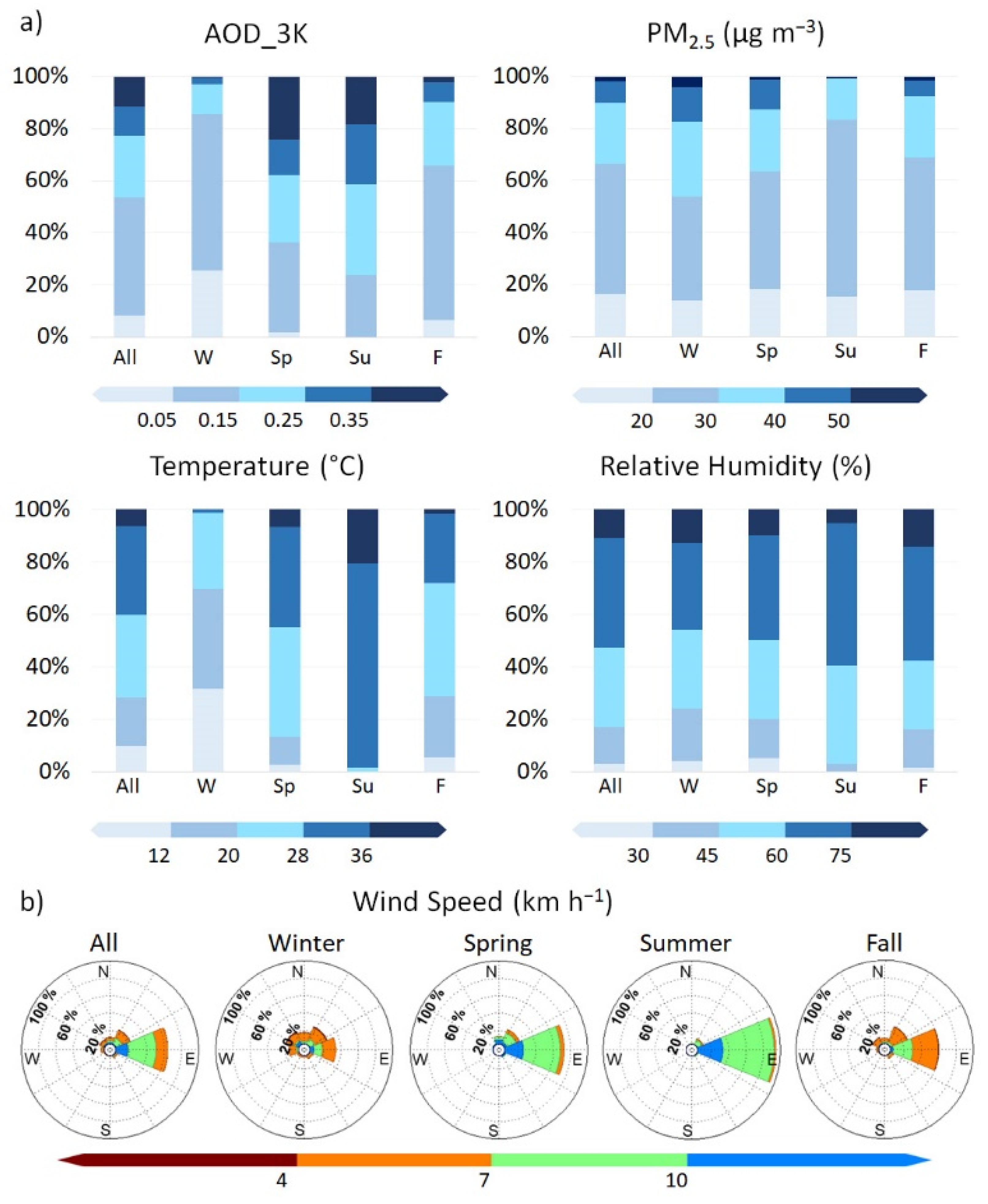
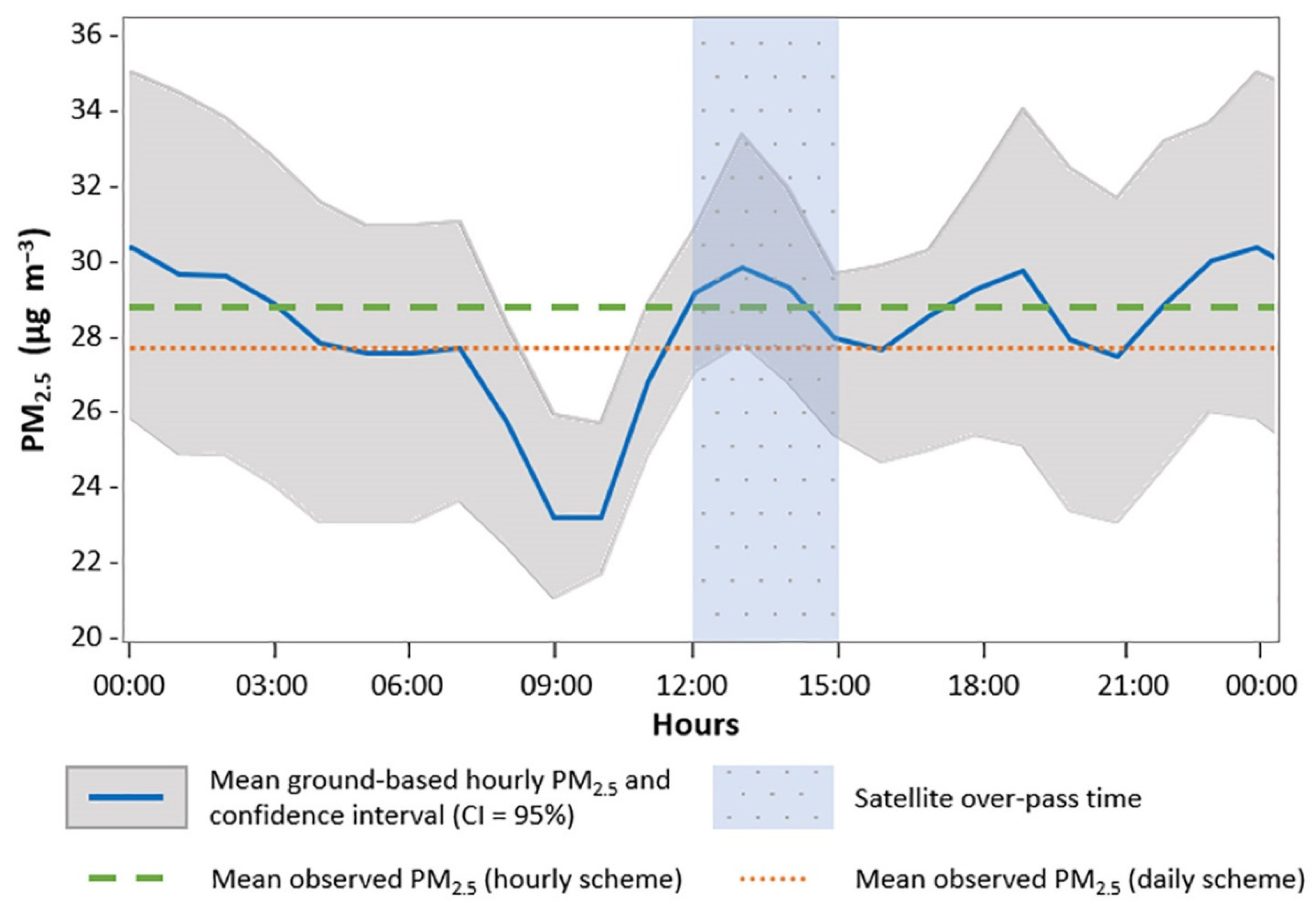
3.3. Model Selection and General Seasonal Variation of the Relevant Variables

Due to its high correlation coefficient, low error estimators, and high data availability, the refined dataset MLR_1 in D3 using the daily scheme was selected in this study as the best dataset. The data distribution of the variables in the best dataset is shown in Figure 4. In general, PM_2.5 and the meteorological variables displayed behavior typical of the region [32,53].

The ground-based temperature (Figure 4a) increased from April to August. July and August were the hottest months, with mean daily maximum and minimum temperatures of 33 °C and 25 °C, respectively. December and January were the coldest months according to the mean daily maximum (22 °C) and minimum (3 °C) temperatures. The RH showed peak daily mean values above 75% in July and above 96% on a few days in December. The predominant wind pattern in the MMA was east to west (Figure 4b). During spring and summer, the WS reached its maximum values of greater than 10 km h⁻¹. Minimum wind speeds of approximately 3–4 km h⁻¹ occurred in the winter and fall seasons, blowing mainly from the northeast and only blowing from the northwest 10% of the days.

The ground-measured PM_2.5 and AOD_3K showed seasonal differences (Figure 4a). The highest observed daily-average PM_2.5 concentrations occurred in winter (64.0 μg m⁻³), whereas the highest AOD_3K was reported in spring (0.89). In winter, cold weather and the corresponding increase in emissions from combustion processes, low mixing heights, and general stagnant conditions resulted in high surface PM_2.5; however, these same meteorological conditions limited the dispersion of fine PM to the free troposphere (above the mixing layer), where there appeared to be low loadings of aerosols as represented by AOD. The latter may also be partially explained by the transit of cold fronts from the north, typical of this season, that help to clean the upper atmosphere (on average, from September to May, 50 cold fronts traverse the region, with the most intense occurring during January and February [54]). Therefore, in winter, the aerosol load integrated over the entire column was low.

The opposite occurs during spring, when the mixing layer height increases substantially; secondary aerosol production is enhanced as a result of higher temperatures and solar radiation, the surface wind intensity increases, and transport is larger (to and from the MMA). Spring is also a period when forest fires occur in the region. In general, spring and early summer are dry periods, increasing dust resuspension. Therefore, aerosol production and transport are enhanced over the entire atmospheric column, which could explain the AOD peak observed in spring. The surface-level PM_2.5 was at its lowest levels in summer; however, high AOD levels were still reported in summer. During this time, the surface wind speed, temperatures, and mixing heights were at their highest values. Accumulation of air pollutants does not occur over the MMA; however, transport effects result in a fair load of aerosols being present throughout the column. Fall is characterized as the rainy season, and therefore, its AOD level is lower than those in spring and summer.

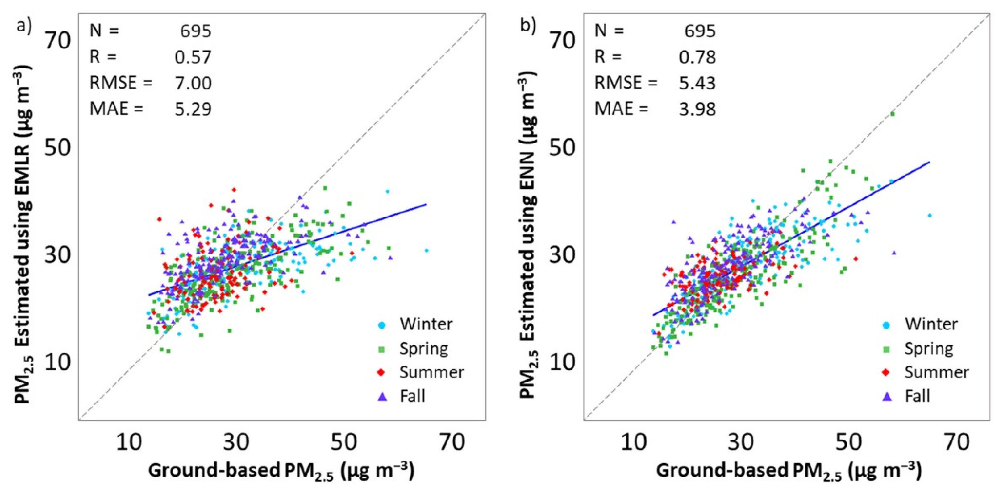
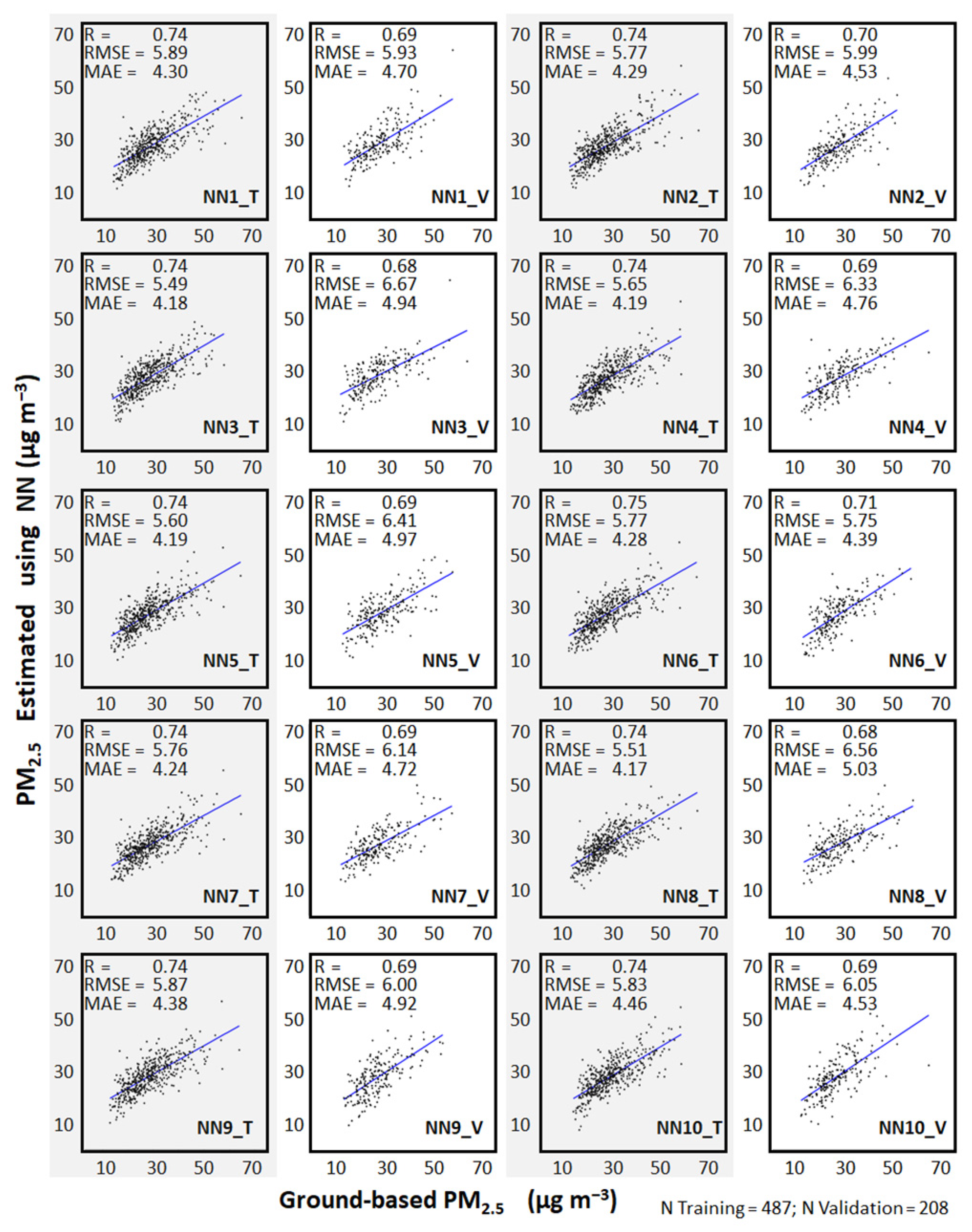
3.4. Performance of the Ensemble Models

The regression coefficients (${\mathsf{\beta }}_i$) obtained from each iteration during the EMLR procedure as well as ${\mathsf{\beta }}_i$ of the EMLR and MLR models using the best dataset (as defined in Section 3.3) are shown in

Table 4. Ensemble model development and comparison with MLR using the original best dataset.

		AOD_3K	T	RH	WS	U	V
	β0	β1	β2	β3	β4	β5	β6
Iteration 1	18.24	+24.21	+0.32	+0.16	−0.84	−11.48	+2.53
Iteration 2	20.67	+22.92	+0.21	+0.16	−0.83	−11.41	+2.98
Iteration 3	21.05	+24.63	+0.24	+0.14	−0.91	−9.99	+2.53
Iteration 4	19.64	+24.68	+0.28	+0.15	−0.83	−12.37	+3.30
Iteration 5	19.82	+20.99	+0.30	+0.16	−0.95	−10.58	+2.48
Iteration 6	17.58	+23.05	+0.28	+0.17	−0.75	−11.31	+2.90
Iteration 7	17.90	+25.21	+0.23	+0.20	−0.72	−12.61	+4.63
Iteration 8	21.19	+26.62	+0.22	+0.15	−0.96	−11.05	+2.63
Iteration 9	18.81	+28.08	+0.23	+0.15	−0.67	−11.40	+3.35
Iteration 10	19.16	+22.20	+0.28	+0.17	−0.80	−12.25	+4.50
Ensemble	19.41	+24.26	+0.26	+0.16	−0.83	−11.45	+3.18
Non-ensemble	19.40	+23.80	+0.26	+0.16	−0.80	−11.60	+3.51

. A one-way ANOVA revealed no statistically significant differences (p-value ≈ 0.97) between the PM_2.5 values estimated from the conventional MLR (95% confidence intervals for the mean: 27.48–28.20) and those estimated using EMLR (95% confidence intervals for the mean: 27.47–28.19). Therefore, performing MLR using the best dataset is robust and the dataset does not influence the model performance.

Because it is appropriate to use the best dataset to enhance the PM_2.5 estimation, 10 trained and validated NNs were used to construct the ENN. Figure 5 shows the statistical performance of each NN. In the training fittings, the R values ranged between 0.74 and 0.75, whereas in the validation datasets, the R values ranged between 0.68 and 0.71. The differences between the R values of the training fittings and those of the validation datasets ranged between 0.04 and 0.06. The differences in RMSE ranged from −1.18 μg m⁻³ to 0.02 μg m⁻³, and the differences in the MAE ranged from −0.87 μg m⁻³ to −0.07 μg m⁻³. These results suggest that the model was not substantially overfitted.

The ground-based PM_2.5 and the EMLR-estimated PM_2.5 (Figure 6a) exhibited a moderate but statistically significant correlation at the 95% confidence level (R = 0.57, RMSE = 7.00 μg m⁻³, and MAE = 5.29 μg m⁻³). The ENN model improved the EMLR PM_2.5 estimations (Figure 6b), with the following performance: R = 0.78, RMSE = 5.43 μg m⁻³, and MAE = 3.98 μg m⁻³.

4. Discussion

4.1. Spatial and Temporal Variability

The use of collocated sites, a widely employed method for estimating PM_2.5 using satellite-derived AOD data (e.g., [55,56]), was not useful for the region of interest, where the MODIS AOD values were irregularly distributed in space and time. In areas with highly heterogeneous surface coverage, as is the case for the MMA, the retrieval frequency of AOD is still a challenge at fine resolutions (D1 and D2). Still, there is potential for the use of the averaged AOD for local and regional PM_2.5 estimations (D3).

Moreover, cloud cover can also affect PM_2.5 assessments because satellite retrieval methods based on solar reflectance depend on the availability of clear sky, in contrast to ground-based monitors, which measure PM concentrations regardless of the cloud conditions [55]. Even though cloud cover data are not routinely reported for the MMA, previous studies suggest that there is a seasonal cloud cover prevailing pattern as easterly anticyclonic air masses highly influence the MMA and are commonly associated with clear sky conditions [57], primarily during the spring and summer months [53].

Furthermore, there is a spatial and temporal mismatch between the averaged satellite AOD and the averaged ground-based PM_2.5 [58]. The correlation between AOD and the ground-based PM_2.5 varies with temporal averaging and geographic location, as shown in Shin et al. (2019) [7]. However, the moderate correlation observed in this study may have been influenced by the relatively low AOD data availability. The results indicate that the data availability increases when the size of the domain increases, with D3 providing the best AOD data representativeness. Therefore, the data availability depends on the spatial scheme rather than the temporal scheme. The correlation coefficient and error estimators depend on both the spatial and temporal schemes; however, the correlation coefficients change significantly as a function of the box size (i.e., errors are larger for the smallest domain), and are larger when using the hourly scheme as opposed to the daily scheme. In summary, the correlation between PM_2.5 and AOD, to some extent, depends on the spatial and temporal average schemes of MODIS AOD [59].

A one-way ANOVA revealed that there was a statistical difference (p-value < 0.05) between the observed hourly-averaged PM_2.5 values (29.39 ± 12.32 µg m⁻³) and the observed daily-averaged PM_2.5 values (27.88 ± 8.52 µg m⁻³). It was observed that the 24-h averages used in the daily scheme suppressed the extreme PM_2.5 values observed in the hourly scheme. The mean and standard deviation of the MLRs performed for the 24 refined datasets were in the same range as the observed dataset for both the hourly and daily schemes. Nonetheless, in this study, the use of a daily scheme yielded the best correlation coefficients in contrast to the study of Guo et al. (2017) [59], in which it was concluded that the best model performance was achieved under an hourly scheme.

The best dataset includes 695 days with valid surface and satellite data. The hourly ground-based PM_2.5 concentrations were averaged, displaying a multimodal pattern (Figure 7), with peaks between 12:00 and 14:00 (likely due to air pollutant emissions and secondary formation), between 18:00 and 20:00 (likely due to emissions during the evening traffic rush-hour), and between 23:00 and 01:00 (possibly due to a decrease in the mixing layer height). The minimum averaged concentration occurred between 08:00 and 10:00. Although traffic emissions increase at morning rush hour (7:00–9:00 h), an increment in the average PM_2.5 concentration was observed starting at 10:00, probably due to the formation of secondary organic aerosol (SOA) and other secondary species (i.e., sulfates) enhanced by photochemical activity. For example, in the MMA, SOA can represent as much as 59% of the PM_2.5, as reported by Mancilla et al. (2015) [60]. For most hours (except between 08:00 and 10:00), the mean ground-based PM_2.5 of the hourly and daily scheme are within the confidence interval of the ground-based hourly PM_2.5. This might explain why, even though AOD was reported only at the satellite overpass time (between 12:00 and 15:00), good statistical performance was achieved when using the daily scheme. However, this might not be the case for all regions and datasets.

4.2. Seasonal Variation in the Model Performance

The EMLR model tended to underestimate the higher ground-based PM_2.5 concentrations and overestimate the lower concentrations. However, the use of ENN reduced the under and over-estimation gap. Similar to our findings, Gupta and Christopher (2009a and 2009b) [61,62] and Zaman et al. (2017) [63] found that NN models improved PM estimations when compared to linear models.

Regarding the error metrics, RMSE was larger than MAE, presumably as a result of the influence of high PM_2.5 episodes in the MMA that were underestimated by the models such as those that occurred in winter. The meteorological conditions in winter can be unfavorable to pollutant dispersion/removal and include frequent occurrences of stagnant weather associated with high pressures, temperature inversion, and diminished precipitation. In addition, the poor air quality in winter is often attributed to large air pollutant emissions resulting from enhanced fossil fuel use for heating purposes [64].

In this study, different seasonal patterns were found between the ground-based PM_2.5 and MODIS AOD correlations, which might arise from their complex relationship as influenced by the aerosol types, aerosol chemical compositions, aerosol size distributions, aerosol vertical profiles, and meteorology [47,65,66,67].

To further explore the observed seasonal variations in the model performance, the fittings from the EMLR and ENN models were divided into four subsets corresponding to each season: winter (December, January, and February), spring (March, April, and May), summer (June, July, and August), and fall (September, October, and November). The model fittings for both EMLR and ENN exhibited a large degree of seasonal variability (Figure 8). The ENN model (R = 0.80, 0.85, 0.51, and 0.72 in winter, spring, summer, and fall, respectively) performed better than the EMLR model (R = 0.65, 0.67, 0.29, and 0.59 in winter, spring, summer, and fall, respectively) for all seasons.

Both the EMLR and ENN models performed better in winter and spring when using seasonal subsets compared to the entire dataset (Figure 6), as found in Li et al., 2017 [68]. The models achieved their lowest performance in summer. During summer, the AOD–PM_2.5 relationship may be influenced by the winds reaching maximum speeds greater than 10 km h⁻¹ (Figure 4b), enhancing the contribution of dust particles. In addition, Mancilla et al. (2019) [32] found that in summer, geological material accounted for 45% of the chemical composition of coarse particles (PMc = PM₁₀ − PM_2.5) and 6% of PM_2.5, suggesting the presence of dust in the MMA atmosphere. Large amounts of atmospheric dust might result in high AOD values [69]. Mancilla et al. (2019) [32] also reported that (NH₄)₂SO₄ can contribute to as much as 54% of the total mass of PM_2.5 in the MMA. According to Gao and Zhang (2014) [70], the extinction coefficient increases with increased SO₂⁻⁴, therefore yielding larger AOD values, as it is the integral of the aerosol extinction coefficient. This also implies that AOD values are influenced not only by aerosol concentrations, but also by aerosol chemical composition.

Estimation of PM_2.5 absolute values using AOD is still a challenge and can be uncertain due to meteorological and seasonal conditions, location (e.g., near major roadways or industrial complexes), or aerosol composition. However, the use of AOD for classifying relative values and categories has been demonstrated to be useful in applications based on pollution concentration intervals rather than absolute values (e.g., public health assessment studies, Air Quality Index), and warrants further research [71].

4.3. Contributions in the Context of Latin America

As stated earlier, few studies have been conducted in the Latin American region to establish the relationship between AOD and PM_2.5. The results obtained here show the feasibility of using averaged satellite-derived AOD for local and regional ground-level PM_2.5 estimations and reinforce the assumption that spatiotemporal variations in the AOD–PM_2.5 relationship need to be understood on a region-by-region basis.

For example, Guevara-Luna et al. (2018) [18] correlated MODIS AOD at 1° resolution (111 km) downloaded from the GIOVANNI online interface and the monthly average surface measurements (2000–2015) for three Colombian cities (Bogota, Medellin, and Bucaramanga) and obtained correlation coefficient R values of over 0.4. Aparicio et al. (2019) [16] used MODIS MOD09CMA AOD data with a spatial resolution of 0.05° as a pollution proxy in La Paz, Lima, and Bogota, by qualitatively comparing AOD and PM₁₀ data.

Téllez-Rojo et al. (2020) [19] used MODIS Multiangle Implementation of Atmospheric Correction (MAIAC) data with a spatial resolution of 1 km, along with interpolated PM_2.5 measurements from Mexico City monitoring network stations, to derive PM_2.5 estimates from a hybrid spatiotemporal model, and reconstruct long- and short-term spatially resolved population exposure to PM_2.5 for epidemiological studies [72]. Their model performance was good even for days without AOD values (cross-validated R² = 0.72 and RMSE = 5.42 µg/m³). In addition, Vu et al. (2019) [20] combined AOD 1-km spatial resolution data retrieved using the MAIAC algorithm, meteorological fields from the European Center for Medium-Range Weather Forecasts, parameters from the Weather Research and Forecasting model coupled with chemistry, and land use variables to fit a random forest (RF) model against ground measurements from 16 monitoring stations, with the objective of developing a PM_2.5 exposure model for Lima, Perú. The RF model performance was as follows: cross-validated R² = 0.70 and RMSE = 5.95 µg/m³, indicating a good fit between the predictors and the ground measurements.

Recently, Santos-Damascena et al. (2021) [73], when performing a multi-country assessment of urban health determinants in Latin America, characterized PM_2.5 levels in 366 cities using satellite-derived estimates. Their study used data from the Atmospheric Composition Analysis Group of Dalhousie University and examined high-resolution AOD-derived from the MAIAC algorithm as a predictor of ground-level PM concentrations in the Metropolitan Area of Sao Paulo (MASP). Correlations between the ground-level PM₁₀ concentrations (at the hour of the satellite overpass, diurnal averaging, and daily averaging intervals) and the collocated AODs were found to be weak (ranging from −0.20 to 0.03), in accordance with a previous study by Natali (2008) [74]. Santos-Damascena et al. (2021) [73] concluded that high-resolution AOD data from the current MAIAC version were not well suited to predict ground-level PM concentrations in the MASP. However, to increase confidence in their conclusions, they compared 2012–2017 AOD retrievals from the DT algorithm at 3 km × 3 km (collection 6.1) with those from an AERONET site and obtained strong correlations for the Terra and Aqua retrievals (R = 0.83 and 0.88, respectively) that were comparable to those obtained for the MAIAC retrievals. The findings of Santos Damascena et al. (2021) [73] suggest that AOD does not necessarily correlate with PM_2.5; therefore, there can be other factors influencing this relationship.

In northeastern Mexico, only Carmona et al. (2020) [17] has evaluated the ability of MERRA-2 aerosol components to represent PM_2.5 ground concentrations and to develop and validate an ENN model to estimate monthly average PM_2.5 ground concentrations. The results of their comparison between the ENN and ground measurements were as follows: R = ~0.90, RMSE = 1.81 μg m⁻³, and MAE = 1.31 μg m⁻³. Apart from comparing four algorithms, this study differs from that of Carmona et al. in having a better temporal resolution (hourly and daily) and using the local meteorology.

5. Conclusions

The AOD–PM_2.5 relationship is complex and, as observed in other regions of the world, for northeastern Mexico, it requires a local assessment of different spatiotemporal averaging schemes to obtain the best correlation. Our results also indicate the need to incorporate other surface-level measured meteorological parameters as predictor variables in addition to AOD to better estimate the PM_2.5 levels. Using the AOD_3K MODIS product (based in the DT algorithm), a 24-h average (daily scheme) over D3 (0.500° × 0.625°) was selected as the dataset that best estimated PM_2.5 concentrations in the MMA as a result of its larger data availability and the mixture of aerosols present in this domain. In addition, the DT algorithm is best suited for NDVI > 0.30, which is typical of vegetative coverage, the dominant coverage in D3. This best dataset was used to develop and validate robust EMLR and non-overfitted ENN models.

The EMLR and ENN models developed here were able to estimate the PM_2.5 concentrations relatively well compared to other applications. In general, the models overpredicted the lowest PM_2.5 concentrations and underpredicted the highest concentrations; this was most evident when using EMLR. Overall, ENN showed better statistical performance than EMLR. When the predicting models were constructed by season, better statistical performances were obtained. The best performance was obtained for seasons with calm or relatively calm winds and low to mild temperatures (winter and spring). The worst performance was observed in summer, when the high winds promote long-range transport and dust resuspension is enhanced, influencing the entire aerosol column. As new retrieval algorithms (with regional calibration), collections, and machine-learning techniques become available, improved performances should be attained.

The methodologies and models developed in this study can help assess local and regional distributions of PM_2.5 in the MMA, improving the knowledge and understanding of the performance of MODIS AOD–PM_2.5 retrieval algorithms over urban, mixed-use land coverage areas with limited ground-based observations, address information gaps, help improve understanding of the exposure–response relationships associated with PM_2.5, and serve as a stepping stone toward designing effective environmental regulations.

References

1. Falcon-Rodriguez, C.I.; Osornio-Vargas, A.R.; Sada-Ovalle, I.; Segura-Medina, P. Aeroparticles, composition, and lung diseases. Front. Immunol. 2016, 7, 3. [Google Scholar] [CrossRef] [Green Version]
2. World Health Organization (WHO). WHO Air Quality Guidelines for Particulate Matter, Ozone, Nitrogen Dioxide and Sulfur Dioxide. Global Update 2005. Summary of Risk Assessment; World Health Organization (WHO): Geneva, Switzerland, 2006. [Google Scholar]
3. United States Environmental Protection Agency (EPA). Section 6.0. Monitoring network design. In QA Handbook; United States Environmental Protection Agency (EPA): Washington, DC, USA, 2008; Volume 2. [Google Scholar]
4. Pinder, R.W.; Klopp, J.M.; Kleiman, G.; Hagler, G.S.; Awe, Y.; Terry, S. Opportunities and challenges for filling the air quality data gap in low- and middle-income countries. Atmos. Environ. 2019, 215, 116794. [Google Scholar] [CrossRef]
5. Gupta, P.; Doraiswamy, P.; Levy, R.; Pikelnaya, O.; Maibach, J.; Feenstra, B.; Polidori, A.; Kiros, F.; Mills, K.C. Impact of California fires on local and regional air quality: The Role of a low-cost sensor network and satellite observations. GeoHealth 2018, 2, 172–181. [Google Scholar] [CrossRef] [PubMed]
6. Van Donkelaar, A.; Martin, R.; Park, R. Estimating ground-level PM2.5 using aerosol optical depth determined from satellite remote sensing. J. Geophys. Res. Space Phys. 2006, 111. [Google Scholar] [CrossRef]
7. Shin, M.; Kang, Y.; Park, S.; Im, J.; Yoo, C.; Quackenbush, L.J. Estimating ground-level particulate matter concentrations using satellite-based data: A review. GISci. Remote Sens. 2019, 57, 174–189. [Google Scholar] [CrossRef]
8. Li, X.; Zhang, C.; Li, W.; Liu, K. Evaluating the use of DMSP/OLS nighttime light imagery in predicting PM2.5 concentrations in the northeastern United States. Remote Sens. 2017, 9, 620. [Google Scholar] [CrossRef] [Green Version]
9. Li, X.; Liu, K.; Tian, J. Variability, predictability, and uncertainty in global aerosols inferred from gap-filled satellite observations and an econometric modeling approach. Remote Sens. Environ. 2021, 261, 112501. [Google Scholar] [CrossRef]
10. Hoff, R.M.; Christopher, S.A. Remote sensing of particulate pollution from space: Have we reached the promised land? J. Air Waste Manag. Assoc. 2009, 59, 645–675. [Google Scholar] [CrossRef]
11. Chu, Y.; Liu, Y.; Li, X.; Liu, Z.; Lu, H.; Lu, Y.; Mao, Z.; Chen, X.; Li, N.; Ren, M.; et al. A review on predicting ground PM2.5 concentration using satellite aerosol optical depth. Atmosphere 2016, 7, 129. [Google Scholar] [CrossRef] [Green Version]
12. Chu, D.A.; Kaufman, Y.J.; Zibordi, G.; Chern, J.D.; Mao, J.; Li, C.; Holben, B.N. Global monitoring of air pollution over land from the earth observing system-terra moderate resolution imaging spectroradiometer (MODIS). J. Geophys. Res. Space Phys. 2003, 108. [Google Scholar] [CrossRef]
13. Engel-Cox, J.; Holloman, C.H.; Coutant, B.W.; Hoff, R.M. Qualitative and quantitative evaluation of MODIS satellite sensor data for regional and urban scale air quality. Atmos. Environ. 2004, 38, 2495–2509. [Google Scholar] [CrossRef]
14. Wang, J.; Christopher, S.A. Intercomparison between satellite-derived aerosol optical thickness and PM2.5 mass: Implications for air quality studies. Geophys. Res. Lett. 2003, 30. [Google Scholar] [CrossRef]
15. Li, J.; Carlson, B.; Lacis, A.A. How well do satellite AOD observations represent the spatial and temporal variability of PM2.5 concentration for the United States? Atmos. Environ. 2015, 102, 260–273. [Google Scholar] [CrossRef]
16. Aparicio, G.; Gerardino, M.P.; Rangel, M.A. Gender gaps in birth weight across Latin America: Evidence on the role of air pollution. J. Econ. Race Policy 2019, 2, 202–224. [Google Scholar] [CrossRef]
17. Carmona, J.M.; Gupta, P.; Lozano-García, D.F.; Vanoye, A.Y.; Yépez, F.D.; Mendoza, A. Spatial and temporal distribution of PM2.5 pollution over northeastern Mexico: Application of MERRA-2 reanalysis datasets. Remote Sens. 2020, 12, 2286. [Google Scholar] [CrossRef]
18. Guevara-Luna, M.A.; Guevara-Luna, F.A.; Mendez-Espinosa, J.F.; Belalcazar-Cerón, L.C. Spatial and temporal assessment of particulate matter using AOD data from MODIS and surface measurements in the ambient air of Colombia. Asian J. Atmos. Environ. 2018, 12, 165–177. [Google Scholar] [CrossRef] [Green Version]
19. Téllez-Rojo, M.M.; Rothenberg, S.J.; Texcalac-Sangrador, J.L.; Just, A.C.; Kloog, I.; Rojas-Saunero, L.P.; Gutiérrez-Avila, I.; Bautista-Arredondo, L.F.; Tamayo-Ortiz, M.; Romero, M.; et al. Children’s acute respiratory symptoms associated with PM2.5 estimates in two sequential representative surveys from the Mexico City metropolitan area. Environ. Res. 2020, 180, 108868. [Google Scholar] [CrossRef]
20. Vu, B.N.; Sánchez, O.; Bi, J.; Xiao, Q.; Hansel, N.N.; Checkley, W.; Gonzales, G.F.; Steenland, K.; Liu, Y. Developing an advanced PM2.5 exposure model in Lima, Peru. Remote Sens. 2019, 11, 641. [Google Scholar] [CrossRef] [PubMed] [Green Version]
21. Park, Y.; Kwon, B.; Heo, J.; Hu, X.; Liu, Y.; Moon, T. Estimating PM2.5 concentration of the conterminous United States via interpretable convolutional neural networks. Environ. Pollut. 2020, 256, 113395. [Google Scholar] [CrossRef] [PubMed]
22. Hu, X.; Waller, L.A.; Al-Hamdan, M.Z.; Crosson, W.L.; Estes, M.G.; Estes, S.M.; Quattrochi, D.A.; Sarnat, J.A.; Liu, Y. Estimating ground-level PM2.5 concentrations in the southeastern U.S. using geographically weighted regression. Environ. Res. 2013, 121, 1–10. [Google Scholar] [CrossRef]
23. Ma, X.; Wang, J.; Yu, F.; Jia, H.; Hu, Y. Can MODIS AOD be employed to derive PM2.5 in Beijing-Tianjin-Hebei over China? Atmos. Res. 2016, 181, 250–256. [Google Scholar] [CrossRef]
24. Ginoux, P.; Deroubaix, A. Space observations of dust in east Asia. In Air Pollution in Eastern Asia: An Integrated Perspective; Bouarar, I., Wang, X., Brasseur, G.P., Eds.; Springer: Berlin, Germany, 2017; pp. 365–383. [Google Scholar]
25. Che, H.; Yang, L.; Liu, C.; Xia, X.; Wang, Y.; Wang, H.; Wang, H.; Lu, X.; Zhang, X. Long-term validation of MODIS C6 and C6.1 Dark Target aerosol products over China using CARSNET and AERONET. Chemosphere 2019, 236, 124268. [Google Scholar] [CrossRef]
26. Consejo Nacional de Población. Delimitación de Las Zonas Metropolitanas de México 2015. 2018. Available online: https://www.gob.mx/conapo/documentos/delimitacion-de-las-zonas-metropolitanas-de-mexico-2015 (accessed on 24 March 2021).
27. INEGI. Censo de Población y Vivienda 2020. 2021. Available online: https://inegi.org.mx/programas/ccpv/2020/ (accessed on 27 May 2021).
28. López-Ramos, E. Geología General y de México; Editorial Trillas: Mexico City, Mexico, 2008; ISBN 978-968-24-1176-2. [Google Scholar]
29. Eguiluz, S.; Aranda, G.M.; Marret, R. Tectónica de La Sierra Madre Oriental, México. Bol. Soc. Geol. Mex. 2000, 53, 1–26. [Google Scholar] [CrossRef]
30. Gobierno de Nuevo León, Secretaria de Desarrollo Sustentable de Nuevo León. Estrategia para la Calidad del Aire de Nuevo León. 2018. Available online: https://www.nl.gob.mx/publicaciones/estrategia-para-la-calidad-del-aire-de-nuevo-leon (accessed on 12 January 2021).
31. Wakamatsu, S.; Kanda, I.; Okazaki, Y.; Saito, M.; Yamamoto, M.; Watanabe, T.; Maeda, T.; Mizohata, A. A Comparative Study of Urban Air Quality in Megacities in Mexico and Japan: Based on Japan-Mexico Joint Research Project on Formation Mechanism of Ozone, VOCs and PM2.5, and Proposal of Countermeasure Scenario; JICA Research Institute: Tokyo, Japan, 2017. [Google Scholar]
32. Mancilla, Y.; Paniagua, I.Y.H.; Mendoza, A. Spatial differences in ambient coarse and fine particles in the Monterrey metropolitan area, Mexico: Implications for source contribution. J. Air Waste Manag. Assoc. 2019, 69, 548–564. [Google Scholar] [CrossRef] [PubMed] [Green Version]
33. Secretaria de Salud. Norma Oficial Mexicana NOM-025-SSA1-2014. Salud Ambiental. Valores Límite Permisibles para la Concentración de Partículas Suspendidas PM10 y PM2.5 en el Aire Ambiente y Criterios para su Evaluación; Secretaria de Salud: Mexico City, Mexico, 2014; p. 20.
34. Blanco-Jiménez, S.; Altúzar, F.; Aguilar, G.; Pablo, M.; Benítez, M.A. Evaluation of suspended particulate matter PM2.5 in the metropolitan area of Monterrey. J. Air Waste Manag. Assoc. 2015, 69, 548–564. [Google Scholar]
35. Mancilla, Y.; Mendoza, A.; Fraser, M.P.; Herckes, P. Chemical characterization of fine organic aerosol for source apportionment at Monterrey, Mexico. Atmos. Chem. Phys. Discuss. 2015, 15, 18. [Google Scholar]
36. Mancilla, Y.; Mendoza, A.; Fraser, M.P.; Herckes, P. Organic composition and source apportionment of fine aerosol at Monterrey, Mexico, based on organic markers. Atmos. Chem. Phys. Discuss. 2016, 16, 953–970. [Google Scholar] [CrossRef] [Green Version]
37. Martinez, M.A.; Caballero, P.; Carrillo, O.; Mendoza, A.; Mejia, G.M. Chemical characterization and factor analysis of PM2.5 in two sites of Monterrey, Mexico. J. Air Waste Manag. Assoc. 2012, 62, 817–827. [Google Scholar] [CrossRef]
38. Mancilla, Y.; Medina, G.; González, L.T.; Mendoza, A. Fine particles emission source profiles for a semi-arid urban center: Key markers and similarity tests. Rev. Int. Contam. Ambient 2021, 6, 237. [Google Scholar]
39. Secretaría de Medio Ambiente y Recursos Naturales. Norma Oficial Mexicana NOM-035-SEMARNAT-1993. Métodos de Medición para Determinar la concentración de Partículas Suspendidas Totales en el Aire Ambiente y los Procedimientos para la Calibración de los Equipos de Medición; Secretaría de Medio Ambiente y Recursos Naturales: Mexico City, Mexico, 1993; p. 18.
40. Secretaría de Medio Ambiente y Recursos Naturales. Norma Oficial Mexicana NOM-156-SEMARNAT-2012, Establecimiento y Operación de Sistemas de Monitoreo de la Calidad del Aire; Secretaría de Medio Ambiente y Recursos Naturales: Mexico City, Mexico, 2012; p. 16.
41. Levy, R.; Mattoo, S.; Munchak, L.A.; Remer, L.A.; Sayer, A.; Patadia, F.; Hsu, N.C. The collection 6 MODIS aerosol products over land and ocean. Atmos. Meas. Tech. 2013, 6, 2989–3034. [Google Scholar] [CrossRef] [Green Version]
42. Hsu, N.C.; Jeong, M.-J.; Bettenhausen, C.; Sayer, A.; Hansell, R.A.; Seftor, C.S.; Huang, J.; Tsay, S.-C. Enhanced deep blue aerosol retrieval algorithm: The second generation. J. Geophys. Res. Atmos. 2013, 118, 9296–9315. [Google Scholar] [CrossRef]
43. Sayer, A.; Munchak, L.A.; Hsu, N.C.; Levy, R.; Bettenhausen, C.; Jeong, M.J. MODIS collection 6 aerosol products: Comparison between aqua’s e-deep blue, dark target, and “merged” data sets, and usage recommendations. J. Geophys. Res. Atmos. 2014, 119, 13. [Google Scholar] [CrossRef]
44. Haykin, S. Neural Networks. A Comprehensive Foundation, 2nd ed.; Pearson Education: Delhi, India, 2005; ISBN 81-7808-300-0. [Google Scholar]
45. Rosenblatt, F. Principles of Neurodynamics. Perceptrons and the Theory of Brain Mechanisms; Spartan Books: Washington, DC, USA, 1962. [Google Scholar]
46. Shepherd, A.J. Second-Order Methods for Neural Networks: Fast and Reliable Training Methods for Multi-Layer Perceptrons; Springer: Berlin, Germany, 1997; p. 145. ISBN 978-1-4471-0953-2. [Google Scholar]
47. Jiang, D.; Zhang, Y.; Hu, X.; Zeng, Y.; Tan, J.; Shao, D. Progress in developing an ANN model for air pollution index forecast. Atmos. Environ. 2004, 38, 7055–7064. [Google Scholar] [CrossRef]
48. Mao, X.; Shen, T.; Feng, X. Prediction of hourly ground-level PM2.5 concentrations 3 days in advance using neural networks with satellite data in eastern China. Atmos. Pollut. Res. 2017, 8, 1005–1015. [Google Scholar] [CrossRef]
49. Sarle, W.S. Stopped training and other remedies for overfitting. In Proceedings of the 27th Symposium on The Interface of Computing Science and Statistics, Pittsburgh, PA, USA, 21–24 June 1995; pp. 352–360. [Google Scholar]
50. Prechelt, L. Automatic early stopping using cross validation: Quantifying the criteria. Neural Netw. 1998, 11, 761–767. [Google Scholar] [CrossRef] [Green Version]
51. Malhotra, R. Empirical Research in Software Engineering: Concepts, Analysis, and Applications; CRC Press: Boca Raton, FL, USA, 2016; ISBN 978-1-4987-1973-5. [Google Scholar]
52. Remer, L.A.; Mattoo, S.K.; Levy, R.C.; Munchak, L.A. MODIS 3 km aerosol product: Algorithm and global perspective. Atmos. Meas. Tech. 2013, 6, 1829–1844. [Google Scholar] [CrossRef] [Green Version]
53. Hernández-Paniagua, I.Y.H.; Clemitshaw, K.C.; Mendoza, A. Observed trends in ground-level O3 in Monterrey, Mexico, during 1993–2014: Comparison with Mexico City and Guadalajara. Atmos. Chem. Phys. Discuss. 2017, 17, 9163–9185. [Google Scholar] [CrossRef] [Green Version]
54. Gobierno de Nuevo León, Protección Civil de Nuevo León. Programa Especial Para La Temporada Invernal 2020–2021. 2020. Available online: https://www.nl.gob.mx/publicaciones/programa-especial-para-la-temporada-invernal-2020-2021 (accessed on 14 May 2021).
55. Christopher, S.; Gupta, P. Global distribution of column satellite aerosol optical depth to surface PM2.5 relationships. Remote Sens. 2020, 12, 1985. [Google Scholar] [CrossRef]
56. Xie, Y.; Wang, Y.; Zhang, K.; Dong, W.; Lv, B.; Bai, Y. Daily estimation of ground-level PM2.5 concentrations over Beijing using 3 km resolution MODIS AOD. Environ. Sci. Technol. 2015, 49, 12280–12288. [Google Scholar] [CrossRef] [Green Version]
57. Jauregui, E. Urban heat island development in medium and large urban areas in Mexico. Erdkunde 1987, 48–51. [Google Scholar] [CrossRef]
58. Kumar, N.; Chu, A.; Foster, A. Remote sensing of ambient particles in Delhi and its environs: Estimation and validation. Int. J. Remote Sens. 2008, 29, 3383–3405. [Google Scholar] [CrossRef] [PubMed]
59. Guo, Y.; Tang, Q.; Gong, D.-Y.; Zhang, Z. Estimating ground-level PM2.5 concentrations in Beijing using a satellite-based geographically and temporally weighted regression model. Remote Sens. Environ. 2017, 198, 140–149. [Google Scholar] [CrossRef]
60. Mancilla, Y.; Herckes, P.; Fraser, M.P.; Mendoza, A. Secondary organic aerosol contributions to PM2.5 in Monterrey, Mexico: Temporal and seasonal variation. Atmos. Res. 2015, 153, 348–359. [Google Scholar] [CrossRef]
61. Gupta, P.; Christopher, S.A. Particulate Matter Air Quality Assessment Using Integrated Surface, Satellite, and Meteorological Products: Multiple Regression Approach. J. Geophys. Res. Space Phys. 2009, 114. [Google Scholar] [CrossRef] [Green Version]
62. Gupta, P.; Christopher, S.A. Particulate matter air quality assessment using integrated surface, satellite, and meteorological products: A neural network approach. J. Geophys. Res. Space Phys. 2009, 114. [Google Scholar] [CrossRef]
63. Zaman, N.A.F.K.; Kanniah, K.D.; Kaskaoutis, D.G. Estimating particulate matter using satellite-based aerosol optical depth and meteorological variables in Malaysia. Atmos. Res. 2017, 193, 142–162. [Google Scholar] [CrossRef] [Green Version]
64. Wang, S.; Zhou, C.; Wang, Z.; Feng, K.; Hubacek, K. The characteristics and drivers of fine particulate matter (PM2.5) distribution in China. J. Clean. Prod. 2017, 142, 1800–1809. [Google Scholar] [CrossRef]
65. Ma, X.; Yu, F. Seasonal variability of aerosol vertical profiles over east US and west Europe: GEOS-Chem/APM simulation and comparison with CALIPSO observations. Atmos. Res. 2014, 140–141, 28–37. [Google Scholar] [CrossRef]
66. Song, Z.; Fu, D.; Zhang, X.; Wu, Y.; Xia, X.; He, J.; Han, X.; Zhang, R.; Che, H. Diurnal and seasonal variability of PM2.5 and AOD in north China plain: Comparison of MERRA-2 products and ground measurements. Atmos. Environ. 2018, 191, 70–78. [Google Scholar] [CrossRef]
67. You, W.; Zang, Z.; Zhang, L.; Li, Y.; Pan, X.; Wang, W. National-scale estimates of ground-level PM2.5 concentration in China using geographically weighted regression based on 3 km resolution MODIS AOD. Remote Sens. 2016, 8, 184. [Google Scholar] [CrossRef] [Green Version]
68. Li, T.; Shen, H.; Zeng, C.; Yuan, Q.; Zhang, L. Point-surface fusion of station measurements and satellite observations for mapping PM2.5 distribution in China: Methods and assessment. Atmos. Environ. 2017, 152, 477–489. [Google Scholar] [CrossRef] [Green Version]
69. Zhang, Y.-L.; Cao, F. Fine particulate matter (PM2.5) in China at a city level. Sci. Rep. 2015, 5, 14884. [Google Scholar] [CrossRef] [PubMed] [Green Version]
70. Gao, Y.; Zhang, M. Modeling study on seasonal variation in aerosol extinction properties over China. J. Environ. Sci. 2014, 26, 97–109. [Google Scholar] [CrossRef]
71. Han, L.; Zhou, W.; Zhao, X.; Li, W.; Qian, Y. Comparing ground operation-measured and remotely sensed fine-particulate matter data: A case to validate the Dalhousie product in China. IEEE Geosci. Remote Sens. Mag. 2019, 7, 20–28. [Google Scholar] [CrossRef]
72. Just, A.C.; Wright, R.; Schwartz, J.; Coull, B.A.; Baccarelli, A.; Tellez-Rojo, M.M.; Moody, E.; Wang, Y.; Lyapustin, A.; Kloog, I. Using high-resolution satellite aerosol optical depth to estimate daily PM2.5 geographical distribution in Mexico City. Environ. Sci. Technol. 2015, 49, 8576–8584. [Google Scholar] [CrossRef] [Green Version]
73. Santos-Damascena, A.; Akemi-Yamasoe, M.; Souza-Martins, V.; Rosas, J.; Rojas-Benavente, N.; Piñero-Sánchez, M.; Ithiro-Tanaka, N.; Nascimento-Saldiva, P.H. Exploring the relationship between high-resolution aerosol optical depth values and ground-level particulate matter concentrations in the metropolitan area of São Paulo. Atmos. Environ. 2021, 244, 117949. [Google Scholar] [CrossRef]
74. Natali, L. The Use of Remote Sensing Products to Characterize Air Quality in São Paulo Metropolitan Region. Master’s Thesis, University of São Paulo, São Paulo, Brazil, 2008. [Google Scholar]
Figure 1. Study area location, ground-based data, and the moderate-resolution imaging spectroradiometer (MODIS) aerosol optical depth (AOD) spatial collocation. (a) The State of Nuevo León (shown in red) is located in northeastern Mexico. (b) The Monterrey Metropolitan Area (MMA) is the main urban area in the state of Nuevo León. (c) Three spatial domains were used D1, D2, and D3. An example of AOD distribution using the MYD04_3k MODIS product (AOD_3K) covering the three domains (D1, D2, and D3) for the period 2010 to 2017 is also shown.
Remotesensing 13 03102 g001
Figure 2. Methodological framework for PM2.5 estimations in the MMA.
Remotesensing 13 03102 g002
Figure 3. Schematic of the neural network (NN) used in this study for estimation of particulate matter with an aerodynamic diameter of less than or equal to 2.5 μm (PM2.5).
Remotesensing 13 03102 g003
Figure 4. Seasonal data distribution of the best dataset for the period of 2010–2017: (a) daily mean AOD_3K and ground-based data (PM2.5, temperature, and relative humidity) and (b) wind roses for the ground-based wind speed and wind direction. In panel (a), W indicates winter, Sp indicates spring, Su indicates summer, and F indicates fall.
Remotesensing 13 03102 g004
Figure 5. Statistical performance of each of the 10 NNs used to construct the ensemble NN (ENN) for the estimation of the daily mean PM2.5 using the best dataset over the MMA from January 2010 to December 2017. Training (T) and validation (V) dataset results are presented.
Remotesensing 13 03102 g005
Figure 6. Statistical performance of the (a) ensemble multiple linear regression (EMLR) and (b) ENN models to estimate the daily mean PM2.5 over the MMA from January 2010 to December 2017. The dash line shows the 1:1 line as a reference.
Remotesensing 13 03102 g006
Figure 7. Hourly ground-based PM2.5 concentrations averaged for the same days and domain covered by the best dataset.
Remotesensing 13 03102 g007
Figure 8. Seasonal model performance of ground-based versus estimated PM2.5 concentrations: EMLR model performance (top) and ENN model performance (bottom).
Remotesensing 13 03102 g008