Assessing within-Field Corn and Soybean Yield Variability from WorldView-3, Planet, Sentinel-2, and Landsat 8 Satellite Imagery

Abstract

Crop yield monitoring is an important component in agricultural assessment. Multi-spectral remote sensing instruments onboard space-borne platforms such as Advanced Very High Resolution Radiometer (AVHRR), Moderate Resolution Imaging Spectroradiometer (MODIS), and Visible Infrared Imaging Radiometer Suite (VIIRS) have shown to be useful for efficiently generating timely and synoptic information on the yield status of crops across regional levels. However, the coarse spatial resolution data inherent to these sensors provides little utility at the management level. Recent satellite imagery collection advances toward finer spatial resolution (down to 1 m) alongside increased observational cadence (near daily) implies information on crops obtainable at field and within-field scales to support farming needs is now possible. To test this premise, we focus on assessing the efficiency of multiple satellite sensors, namely WorldView-3, Planet/Dove-Classic, Sentinel-2, and Landsat 8 (through Harmonized Landsat Sentinel-2 (HLS)), and investigate their spatial, spectral (surface reflectance (SR) and vegetation indices (VIs)), and temporal characteristics to estimate corn and soybean yields at sub-field scales within study sites in the US state of Iowa. Precision yield data as referenced to combine harvesters’ GPS systems were used for validation. We show that imagery spatial resolution of 3 m is critical to explaining 100% of the within-field yield variability for corn and soybean. Our simulation results show that moving to coarser resolution data of 10 m, 20 m, and 30 m reduced the explained variability to 86%, 72%, and 59%, respectively. We show that the most important spectral bands explaining yield variability were green (0.560 μm), red-edge (0.726 μm), and near-infrared (NIR − 0.865 μm). Furthermore, the high temporal frequency of Planet and a combination of Sentinel-2/Landsat 8 (HLS) data allowed for optimal date selection for yield map generation. Overall, we observed mixed performance of satellite-derived models with the coefficient of determination (R²) varying from 0.21 to 0.88 (averaging 0.56) for the 30 m HLS and from 0.09 to 0.77 (averaging 0.30) for 3 m Planet. R² was lower for fields with higher yields, suggesting saturation of the satellite-collected reflectance features in those cases. Therefore, other biophysical variables, such as soil moisture and evapotranspiration, at similar fine spatial resolutions are likely needed alongside the optical imagery to fully explain the yields.

1. Introduction

Crop yield assessment and forecasting is one of the major components in agriculture production monitoring [1]. Timely, accurate, and spatially explicit information on crop yields at global, national, and regional scales is extremely important [2] for understanding and allocating the food supply. Furthermore, spatial variability of crop yields at the field scale can help provide objective information to farmers to improve management practices and identify yield gaps [3,4,5] or to improve insurance companies’ risk models [6].

The increased number of very high spatial resolution (VHR, <5 m) sensors onboard space-borne platforms, including micro and nanosatellites, are providing opportunities for a new generation of spatially detailed geo-information products for agricultural monitoring. High temporal resolution (near daily cadence) is additionally required for agricultural applications to monitor and capture the dynamics of crop growth [7,8,9,10]. Images acquired by the WorldView-3 (WV-3, ~1.25 m) satellite or the PlanetScope (Dove-Classic, ~3 m) constellation of satellites have finer spatial resolution compared to images provided by moderate spatial resolution satellites such as Landsat 8 (30 m) [11] and Sentinel-2 (10–20 m) [12]. While WV-3 provides better spatial resolution and richer spectral information in visible and near-infrared (NIR) spectrum (eight bands vs. four) compared to Planet/Dove, only the latter provides a near-daily revisit cycle.

The combined spatial and temporal attributes from WorldView-3 and Planet can provide new insight on the variability of crop parameters at field scale, including yields [13]. Satellite data availability during the growing season can be used to predict before harvest within-the-field crop yields or analyze areas of higher and lower yields for precision farming. It can also be used for stratification purposes within the sampling-based estimation of yields [14,15]. The latter is especially important, since if satellite data could capture within-field crop variability during the vegetation season, they would allow one to guide, and potentially improve, the sampling strategies for ground-based crop yield estimation and validation.

This is similar to the approach of using satellite-derived classification maps for guiding sampling strategies to estimate areas of land cover land use change (LCLUC) [16,17]. However, in the case of LCLUC, one must deal with categorical information, while in the case of yields, it is continuous information. To address that aspect, dedicated frameworks such as VALidation of European Remote sensing Instruments (VALERI) [18] protocol have been setup to validate satellite-derived maps of biophysical variables from coarse to moderate spatial resolutions. The VALERI protocol introduces an elementary sampling unit (ESU) corresponding to the spatial resolution of a satellite-derived map (e.g., a 30 × 30 m pixel) and a number of point-based measurements (e.g., 10–15 samples per ESU). Thus, the variability of the biophysical parameter inside the ESU can be captured.

Previous studies have attempted to connect remote sensing data (both reflectances and vegetation indices (VIs)) acquired from space-borne VHR sensors with crop yields at field scale and showed promising results [13,19,20,21,22,23]. Most studies used IKONOS, Quickbird, SPOT5, or the RapidEye satellites. Even through VHR, each would only provide one or a few image acquisitions throughout the season, which would bring large uncertainties in terms of optimal timing for correlating satellite-derived features with yields.

Therefore, space-borne sensors at very high spatial and temporal resolution can provide new insights and opportunities for precision agriculture [13,24] and further expand applications of remote sensing sensors in agricultural domains at various geographical scales. The present study takes advantage of VHR satellite data made available within the National Aeronautics and Space Administration’s (NASA) program to explore the strengths and the limitations of multi-spectral sensors to explain crop yield variability at field scale. Specifically, the present study aims to address the following research questions:

• Q1: How does the spatial resolution affect our ability to explain crop yields at field scale?
• Q2: To what degree can crop yield variability at field scale be explained by using space-borne multi-spectral sensors only?
• Q3: What is the optimal timing of satellite image acquisitions and optimal spectral bands for explaining within-field variability?

The study was performed for 2018 and 2019 using VHR data (1–3 m), acquired by PlanetScope (Dove-Classic) and WorldView-3 satellites. Additionally, use comparisons were made to moderate spatial resolution data (30 m) as acquired by Landsat-8 and Sentinel-2 satellites. The crops of corn and soybean were both analyzed with the study sites being within Iowa, US. The within-field ground refence data were precision collected by harvesting machines.

2. Materials and Methods

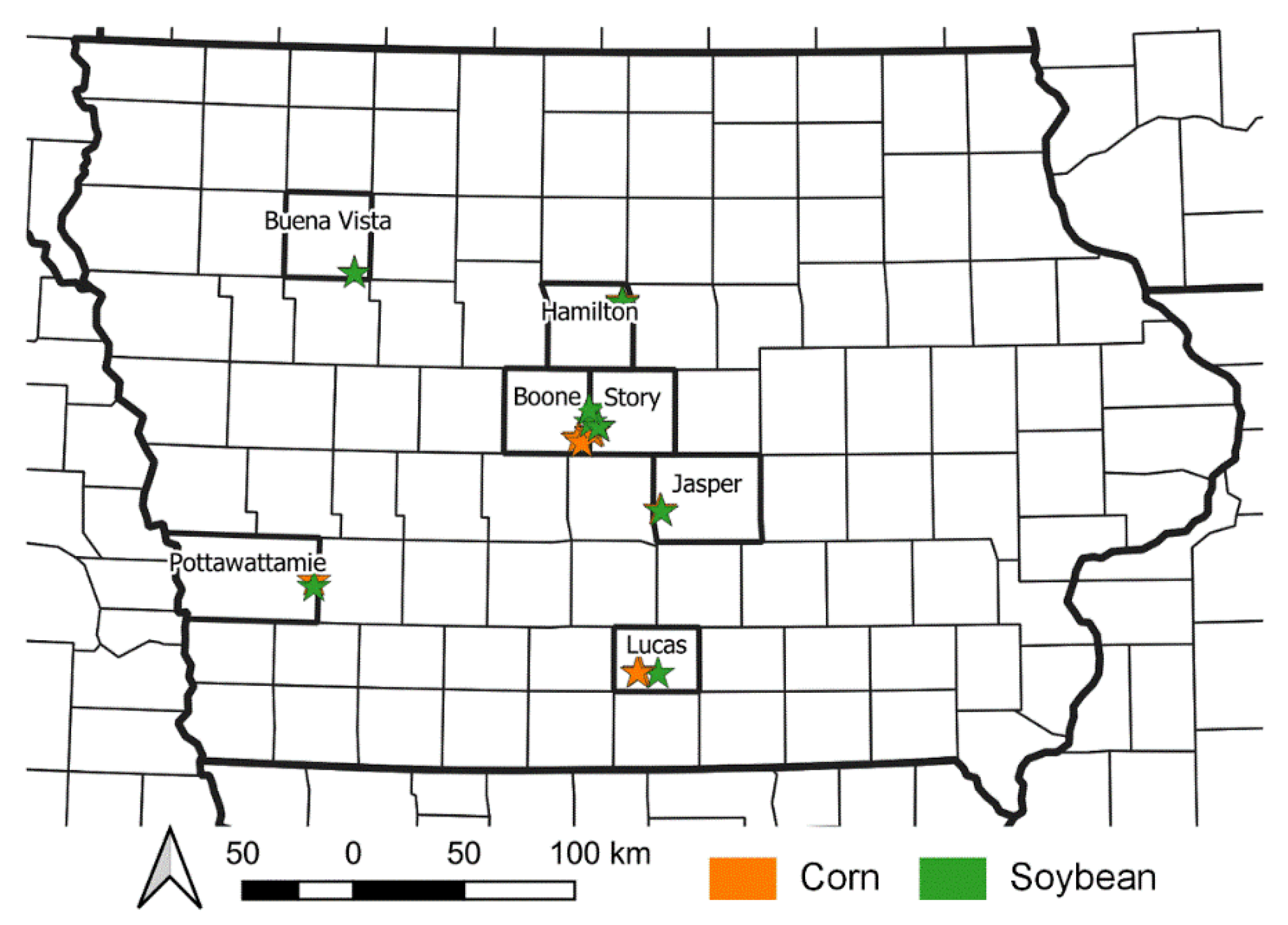
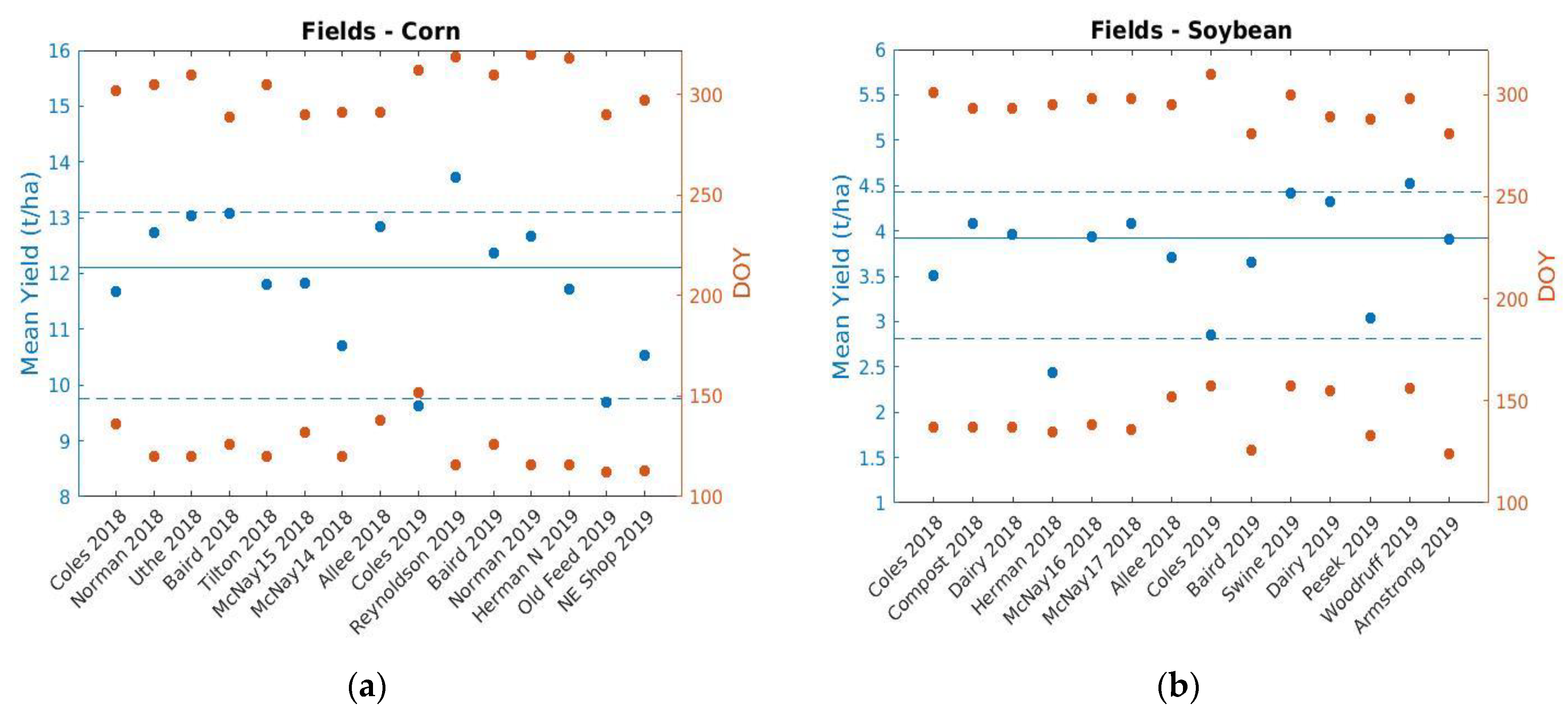
2.1. Study Area and Reference Yield Data

Corn and soybean yields were obtained for 30 fields in 2018 and 2019 from Iowa State University. Fields were scattered throughout 7 counties in the state of Iowa, namely Boone, Buena Vista, Hamilton, Jasper, Lucas, Pottawatomie, and Story (Figure 1). The detailed characteristics of each field are described in

Table A1. Detailed information on corn and soybean fields used in the study. DOY is the day of the year. Shown are per-field average yield and standard deviation (SE).

Field Id	County in Iowa	Latitude, Longitude	Crop	Year	Yield, t/ha	Planting/ Harvesting DOY
Baird	Jasper	41.632, −93.305	Corn	2018	13.1 ± 1.2	126/289
Uthe	Boone	41.931, −93.754	Corn	2018	13.0 ± 1.9	120/310
Allee	Buena Vista	42.586, −95.00	Corn	2018	12.8 ± 0.6	138/291
Norman	Story	41.952, −93.689	Corn	2018	12.7 ± 3.0	120/305
McNay	Lucas	40.956, −93434	Corn	2018	11.8 ± 2.2	132/290
Tilton	Story	41.954, −93.675	Corn	2018	11.8 ± 3.1	120/305
Coles	Hamilton	42.481, −93.523	Corn	2018	11.7 ± 1.2	136/302
McNay	Lucas	40.975, −93.432	Corn	2018	10.7 ± 2.2	120/291
Compost	Story	41.977, −93.656	Soybean	2018	4.1 ± 0.9	137/293
McNay	Lucas	40.979, −93.417	Soybean	2018	4.1 ± 0.6	136/298
Dairy	Story	41.974, −93.648	Soybean	2018	3.9 ± 0.7	137/293
McNay	Lucas	40.972, −93.32	Soybean	2018	3.9 ± 0.6	138/298
Allee	Buena Vista	42.584, −95.00	Soybean	2018	3.7 ± 0.3	152/295
Coles	Hamilton	42.488, −93.523	Soybean	2018	3.5 ± 0.5	157/310
Herman	Boone	41.909, −93.739	Soybean	2018	2.4 ± 0.6	135/295
Reynoldson	Boone	41.925, −93.761	Corn	2019	13.7 ± 1.3	116/319
Armstrong	Pottawatomie	41.329, −95.181	Corn	2019	13.1 ± 2.3	115/293
Norman	Lucas	41.952, −93.689	Corn	2019	12.7 ± 1.6	116/320
Baird	Jasper	41.639, −93.312	Corn	2019	12.4 ± 1.3	126/310
Herman	Boone	41.909, −93.739	Corn	2019	11.7 ± 1.6	116/318
NE Shop	Lucas	40.979, −93.417	Corn	2019	10.5 ± 1.5	113/297
Old Feed	Lucas	40.975, −93.432	Corn	2019	9.7 ± 2.4	112/290
Coles	Hamilton	42.488, −93.523	Corn	2019	9.6 ± 1.4	153/312
Woodruff	Story	41.992, −93.694	Soybean	2019	4.5 ± 1.3	156/298
Swine	Boone	42.048, −93.701	Soybean	2019	4.4 ± 1.1	157/300
Dairy	Story	41.975, −93.649	Soybean	2019	4.3 ± 0.6	155/289
Armstrong	Pottawatomie	41.305, −95.180	Soybean	2019	3.9 ± 0.6	124/281
Baird	Jasper	41.632, −93.305	Soybean	2019	3.6 ± 0.6	126/281
Coles	Hamilton	42.481, −93.523	Soybean	2019	2.8 ± 0.5	157/310
Pesek	Boone	42.043, −93.701	Soybean	2019	3.0 ± 0.4	133/288

. The yield data were collected by combine harvesting machines, which provide dry volumetric yields roughly every three meters along track. These yields were pre-processed before correlating them to the satellite imagery. Headlands, row ends, and samples outside ±3 standard deviations from the field mean were removed. In cases when several data records with different yield values were within 3 m of each other, only the data record with the maximum yield was retained, while others were filtered out [20,25,26].

Average per-field yield values as well as planting and harvest dates are shown in Figure 2. The average yield for corn was 12.1 t/ha and varied from 9.6 t/ha to 13.6 t/ha and for soybean was 3.9 t/ha and varied from 2.4 t/ha to 4.5 t/ha. On average, corn and soybean were planted on 4 May (day of year (DOY) 124) and 23 May (DOY 143). They were harvested on 30 October (DOY 303) and 22 October (DOY 295), respectively. Figure 3 shows an example of within-field yield distribution for Coles corn and soybean fields in 2019.

2.2. Satellite Data

2.2.1. Satellite Data at Very High Spatial Resolution (VHR): WorldView-3 and Planet

WorldView-3 (WV-3) data were provided by the NASA’s Commercial Archive Data for NASA investigators (cad4nasa.gsfc.nasa.gov accessed on 29 January 2021) [27]. WV-3 acquires data of the Earth’s surface in eight spectral bands in the visible and infrared range of electromagnetic spectrum: coastal blue (0.426 μm), blue (0.479 μm), green (0.552 μm), yellow (0.610 μm), red (0.662 μm), red-edge (0.726 μm), and two near-infrared (NIR1 0.831 μm and NIR2 0.910 μm) channels. At-nadir spatial resolution is 1.25 m. WV-3 also acquires data in eight short-wave infrared bands (ranging from 1195 nm to 2365 nm), but those were unavailable and, hence, not used. Since only archival images were selected and no new acquisitions were available, we were able to obtain two WV-3 images over the Coles fields, for which within-fields yields were available (Figure 4). Though the timing of the WV-3 images (2 and 21 July 2018) might not have been optimal, those data were still useful in analyzing WV-3 spectral bands at 1.25 m spatial resolution to explain within-field corn and soybean yield variability early in the season (planting dates were 16 May and 6 June 2018 for corn and soybean, respectively). Images’ digital numbers were converted to the top-of-atmosphere (TOA) reflectance values and further processed for atmospheric correction. We used an adapted version of the Land Surface Reflectance Code (LaSRC), previously developed for the moderate spatial resolution satellites such as Landsat 8 [28] and Sentinel-2 [29]. LaSRC is a generic atmospheric correction algorithm for estimating land surface reflectance (SR), which takes into account absorption by atmospheric gases and scattering by molecules and aerosols. It is based on the inversion of the “6SV” radiative transfer code. The result of the atmospheric correction is the estimate of SR in the corresponding spectral bands of WV-3 satellite.

Planet data, acquired by Dove-Classic sensors, were acquired through the NASA program [30]. PlanetScope is composed of a constellation of satellites that provide a near-daily global coverage of the Earth surface [31]. Dove-Classic sensors acquire data in the four spectral bands: blue (0.485 µm), green (0.545 µm), red (0.630 µm), and near-infrared (0.820 µm) at 3.25 m spatial resolution. We acquired all cloud-free Planet data over the fields for the whole growing season in 2018 and 2019 and an SR product provided by Planet. There were 1167 and 1095 unique scenes, respectively, for those two years.

2.2.2. Satellite Data at Moderate Spatial Resolution: Landsat 8 and Sentinel-2

We used NASA’s Harmonized Landsat Sentinel-2 (HLS, ver. 1.4) product at 30 m [32] to correlate satellite-derived features with crop yields. HLS is an analysis ready data product, which is derived from original TOA reflectance data by applying a series of pre-processing steps, including co-registration, cloud screening, atmospheric and angular corrections, and spectral adjustments. This ensures that data acquired by Landsat 8 and Sentinel-2 satellites are geometrically and radiometrically harmonized and can be used together. Combination of Landsat 8 and Sentinel-2A/B satellites provides a global median average revisit interval of 2.9 days [33] and already proved to be beneficial for crop yield assessment [9]. HLS is organized using a Sentinel-2 tiling system with each tile covering the area of approximately 110 km × 110 km. We used the following tiles, which covered corn and soybean fields in the study region: 15TVH, 15TVG, 15TVF, 15TUH, and 15TUF. We used the following spectral bands: green (wavelength ~0.560 μm), red (~0.660 μm), NIR (~0.865 μm from the 8A band of Sentinel-2), and two short-wavelength infrared (SWIR) (~1.5 and ~2.2 μm). Overall, 407 and 400 unique HLS scenes were used in 2018 and 2019, respectively.

2.3. Methods

First, we explored the effect spatial resolution has on capturing field-scale yield variability. For this, the harvest data from machinery were used to simulate how much yield variability is reduced when spatial resolution decreases. Yield data from the combine machinery were again available approximately every 3 m. Yield maps were generated at spatial resolutions of 10 m, 20 m, and 30 m by averaging all the point yield data within the coarser pixel. Relative efficiency, which is the ratio between yield variance at coarse resolution (10 m, 20 m, or 30 m) to yield variance at 3 m resolution, was used as a numerical metric for yield variability evaluation:

$$R\left(x\right)=\raisebox{1ex}{$V_y\left(x\right)$}\!\left/ \!\raisebox{-1ex}{$V_y\left(x_0\right)$}\right.,$$

(1)

where $R\left(x\right)$ is the relative efficiency at spatial resolution $x$ m, $V_y\left(x\right)$ is the variance of yield at $x$ m, and $x_0=3$ m. This metric is similar to the metric used in land area estimation and in quantifying the efficiency of satellite data in reducing the variance of the area estimates [16,34].

We also used the coefficient of variation (CV) to measure a relative variability of yields within the pixel or a field:

$$CV=100\%\times \frac{{\sigma }_y}{{\mu }_y},$$

(2)

where ${\sigma }_y$ and ${\mu }_y$ are standard deviation and average of yields $y$.

In order to explore the yield variability at field scale, the reference within-field corn and soybean yield values were correlated with the satellite-derived features of SR or VIs using a multivariable linear regression (

Table 1. Vegetation indices used in the study.

Vegetation Index	Formula
Normalized difference vegetation index (NDVI)	$\frac{{\rho }_{NIR }-{\rho }_{RED }}{{\rho }_{NIR}+{\rho }_{RED }}$
Difference vegetation index (DVI)	${\rho }_{NIR }-{\rho }_{RED }$
Enhanced vegetation index (EVI)	$2.5\frac{{\rho }_{NIR }-{\rho }_{RED }}{{\rho }_{NIR}+2.4{\rho }_{RED }+1}$
Green NDVI (GNDVI)	$\frac{{\rho }_{NIR }-{\rho }_{GREEN }}{{\rho }_{NIR}+{\rho }_{GREEN }}$
Green chlorophyll vegetation index (GCVI)	$\frac{{\rho }_{NIR }}{{\rho }_{GREEN }}-1$
Wide dynamic range vegetation index (WDRVI)	$\frac{0.1{\rho }_{NIR }-{\rho }_{RED }}{0.1{\rho }_{NIR }+{\rho }_{RED }}$
Soil-adjusted vegetation index (SAVI)	$\frac{{\rho }_{NIR }-{\rho }_{RED }}{{\rho }_{NIR}+{\rho }_{RED }+L}\left(1+L\right), L=0.33$
Red edge chlorophyll index (CIre) 1	$\frac{{\rho }_{NIR }}{{\rho }_{RED-EDGE }}-1$

¹ For WV-3 data.

). For 1.25 m WV-3 and 3 m Planet data, those features were derived for each yield sample separately, while for 30 m HLS data, those yield values were averaged within each 30 m pixel. Specifically, for each cloud-free satellite acquisition, a linear regression model was built between yields and SRs or VIs, and an adjusted coefficient of determination $R_{\mathrm{adj}}^2$ and a root mean square error (RMSE) were calculated:

$$R^2=1-\frac{{{\displaystyle \sum }}_{i=1}^n{\left(y_{est}-y_{ref}\right)}^2}{{{\displaystyle \sum }}_{i=1}^n{\left({\overline{y}}_{ref}-y_{ref}\right)}^2},$$

(3)

$$R_{\mathrm{adj}}^2=1-\left(1-R^2\right)\frac{n-1}{n-p-1},$$

(4)

$$\mathrm{RMSE}=\sqrt{\raisebox{1ex}{$1$}\!\left/ \!\raisebox{-1ex}{$n$}\right.{{\displaystyle \sum }}_{i=1}^n{\left(y_{est}-y_{ref}\right)}^2},$$

(5)

$$\mathrm{RRMSE}=100\%\times \raisebox{1ex}{$\mathrm{RMSE}$}\!\left/ \!\raisebox{-1ex}{${\overline{y}}_{ref}$}\right.,$$

(6)

where $y_{est}$ and $y_{ref}$ are estimate and reference yield values, respectively; ${\overline{y}}_{ref}=\raisebox{1ex}{$1$}\!\left/ \!\raisebox{-1ex}{$n$}\right.{\displaystyle \sum }_{i=1}^n{y}_{ref}$ is the average of the reference values, n is the number of samples, and p is the number of variables (without the constant term).

For Planet and HLS data, the best date in terms of maximum $R_{\mathrm{adj}}^2$ was determined to correlate with crop yields. For WV-3, no time series was available, thus we focused on exploring various spectral bands using a “feature importance” metric derived from the random forest regression [35]. This was done through multiple random permutations of input features, and regression was evaluated in terms of information gain. Features that provided higher informativeness had a higher importance level.

3. Results

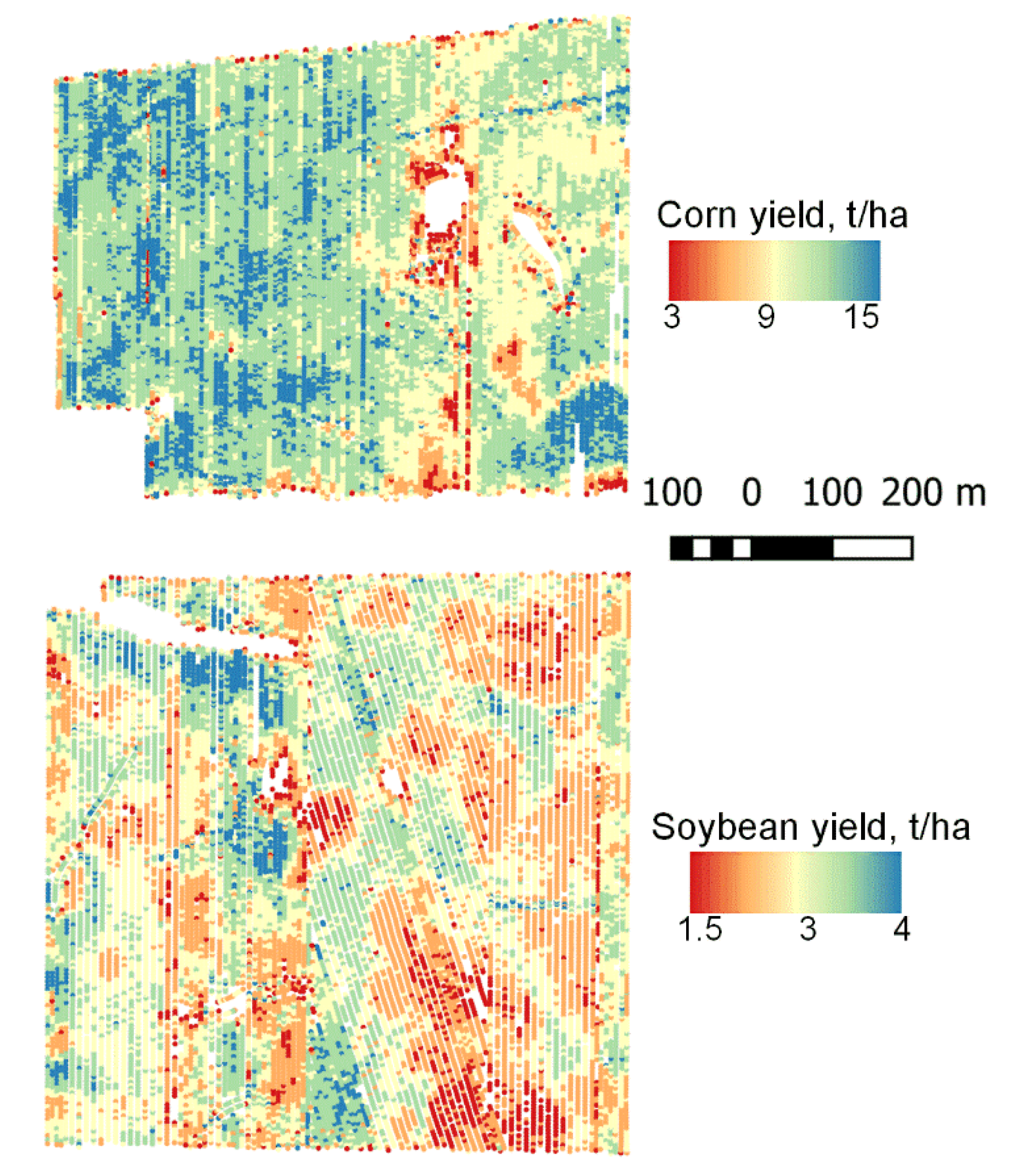
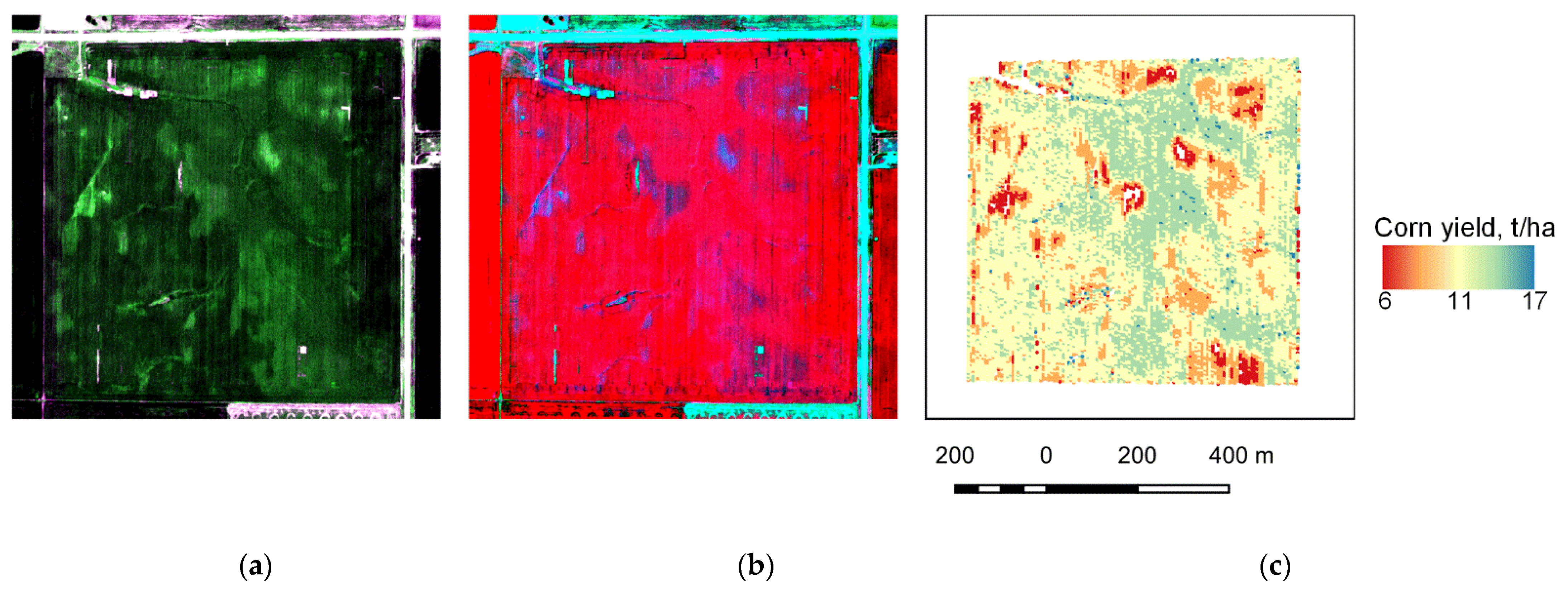
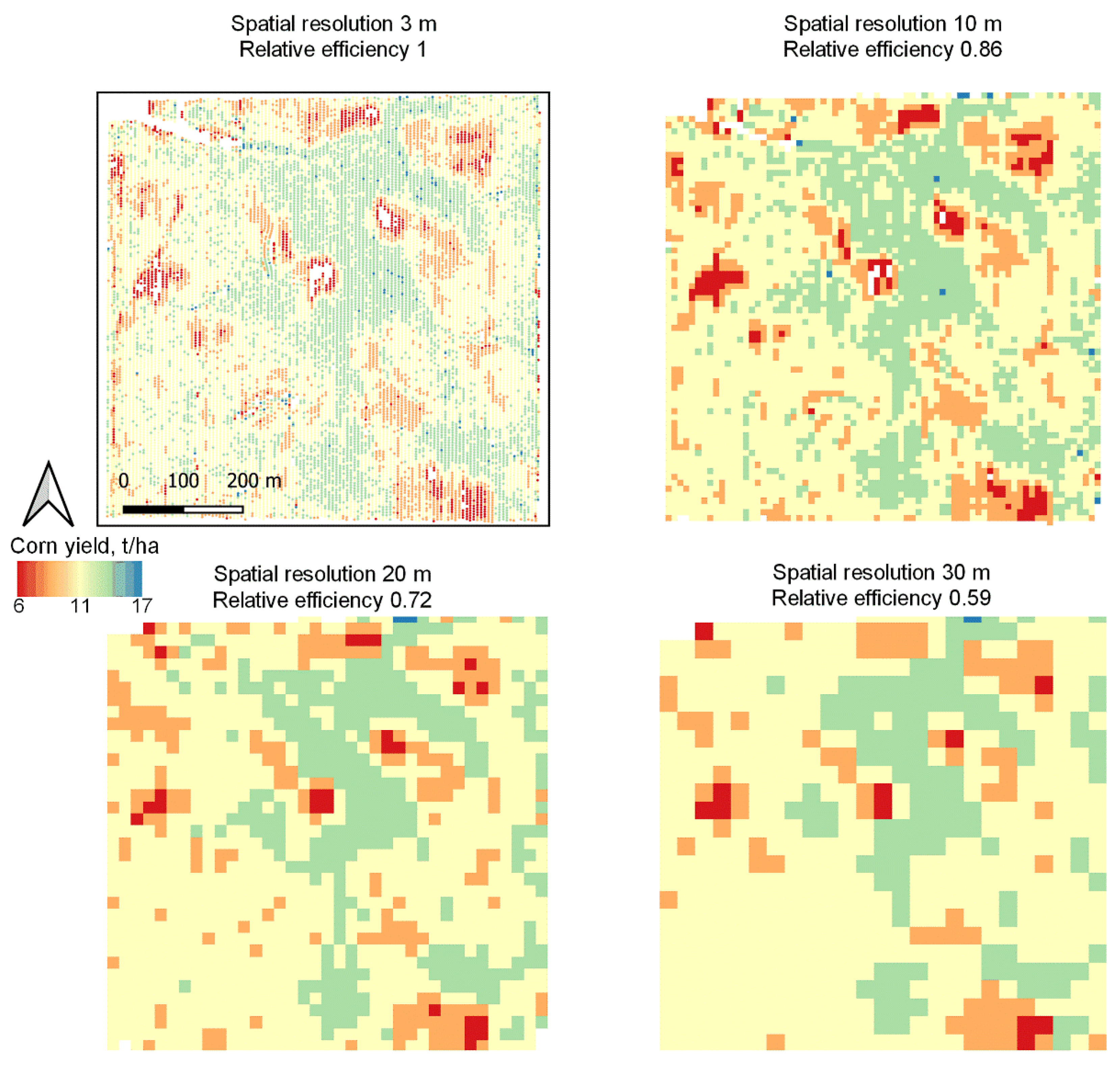
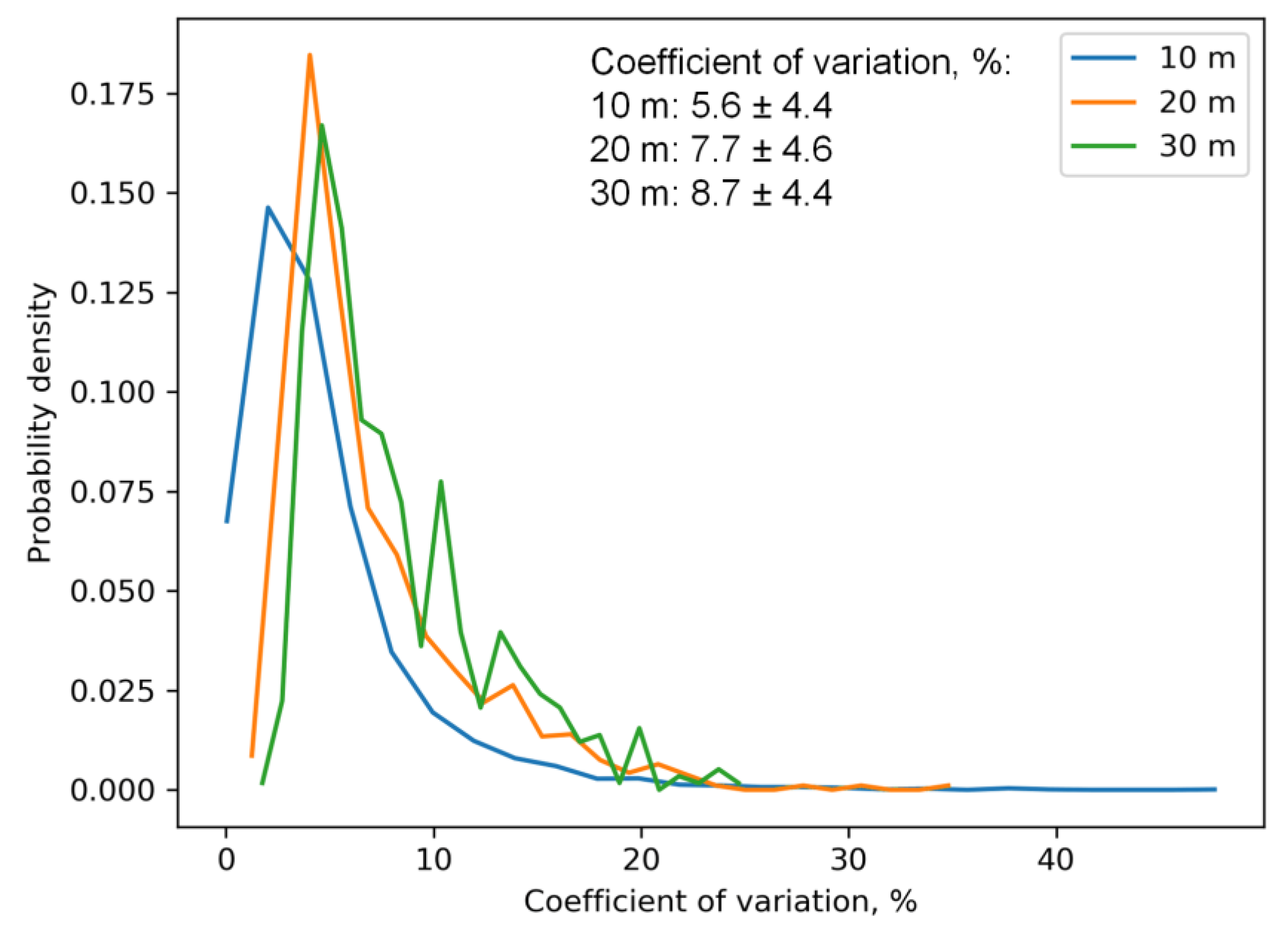
3.1. Effect of Spatial Resolution on Capturing Field Scale Yield Variability

Figure 5 shows the effect of spatial resolution on capturing within-field yield variability using a corn field as an example. These results show the difference between high spatial resolution data compared to moderate spatial resolution of 10–30 m. For example, only 59% of yield variability can be explained with 30 m, while the rest is lost because of coarsening and mixture effects inside the 30 m pixel.

At present, one of the popular approaches for collecting reference crop yields is through the crop cuts [14,15]. At fine spatial scales (usually at less than 1 m), destructive harvesting of the crops is made, and the yield is estimated from the collected grain. Those yields are then used as reference and compared to satellite-derived yields at moderate spatial resolution. However, sampling within the moderate resolution pixel should be statistically rigorous, thus the selected samples would capture yield variability across the moderate resolution pixel, and therefore the estimates would be unbiased. Figure 6 shows a histogram of the CV (Equation (2)) for the yields at 10 m, 20 m, and 30 m resolutions. CV exceeds 20% and 10% at 30 m and 10 m, respectively. Our results are in line with the previously developed VALERI protocol [18]. Therefore, a similar protocol shall be implemented for any sample-based ground measurements of crop yields, when multiple samples should be selected inside a 10 or 30 m pixel to capture yield variability. The VALERI protocol recommends 10–15 samples of in-situ ground measurements of the biophysical variable inside the pixel. One cannot make a single crop cut inside a 30 m pixel and compare to the satellite-derived yields at moderate spatial resolution.

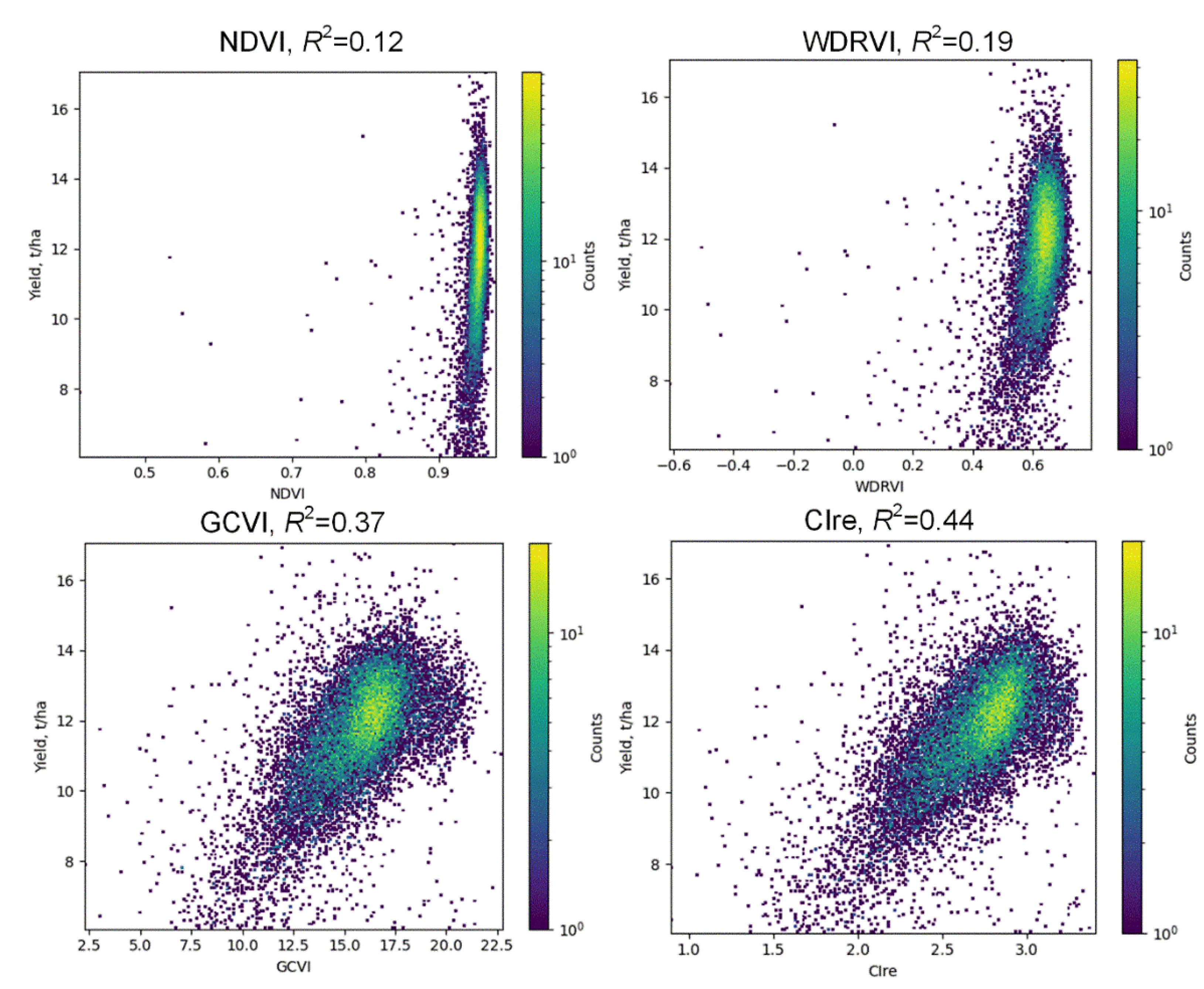
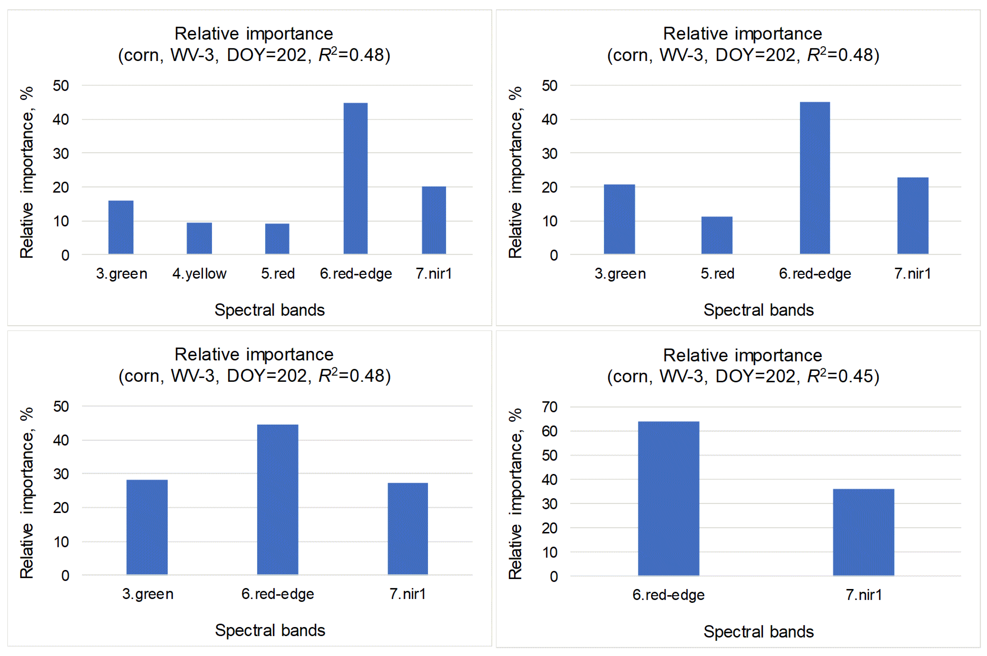
3.2. Analysis of Corn and Soybean Yield Varibility with WV-3 Data

Table 2. Coefficient of determination $R^2$ obtained for the Coles fields for 2018 when using linear models between yields and surface reflectance (SR) values (all spectralas a function of the day of year bands) for the WV-3 images.

Crop	Acquisition Date	${\mathit{R}}^2$	RMSE, t/ha	RRMSE, %
Corn	2 July 2018	0.35	1.23	10.5
Corn	21 July 2018	0.48	1.07	9.2
Soybean	2 July 2018	0.28	0.50	14.2
Soybean	21 July 2018	0.36	0.47	13.2

RMSE: root mean square error (Equation (5)); RRMSE: relative RMSE (Equation (6)).

shows values of the coefficient of determination, RMSE values obtained for the linear models correlating corn and soybean yields, and SR values derived from WV-3 images. A model based on WV-3 image acquired on 21 July 2018 was able to explain 48% of corn (RMSE = 1.07 t/ha or 9.2%) and 36% of soybean (RMSE = 0.47 t/ha or 13.2%) yield variability. This was 66 and 45 days after corn and soybean planting, respectively. The SR-based model outperformed a single-regressor model based on the VI. For corn, the best one was with the red edge chlorophyll index (Cire) and gave R² = 0.44 and RMSE = 1.11 t/ha (9.5%) (Figure 7). For soybean, the best VI-based model was with the difference vegetation index (DVI) and gave R² = 0.25 and RMSE = 0.50 t/ha (14.3%). Overall, VIs based on the red spectral band were not able to explain corn yield variability (the best was Wide dynamic range vegetation index (WDRVI) at 19%), whereas the green-based index Green chlorophyll vegetation index (GCVI) and the red-edge-based index CIre were able to explain 37% and 44% of yield variability, respectively.

Not all spectral bands were equally important in explaining corn and soybean variability. Figure 8 shows performance of various models and relative importance of spectral bands. Results suggest that, during the stage of corn development when a WV-3 image was taken, in this case, 66 days after planting, the red-edge (0.726 µm), the green (0.552 µm), and the NIR (0.831 µm) bands were the most important in explaining yield variance at field scale. These are in accordance with results obtained for VIs, when red-edge and green-based indices outperformed red-based indices.

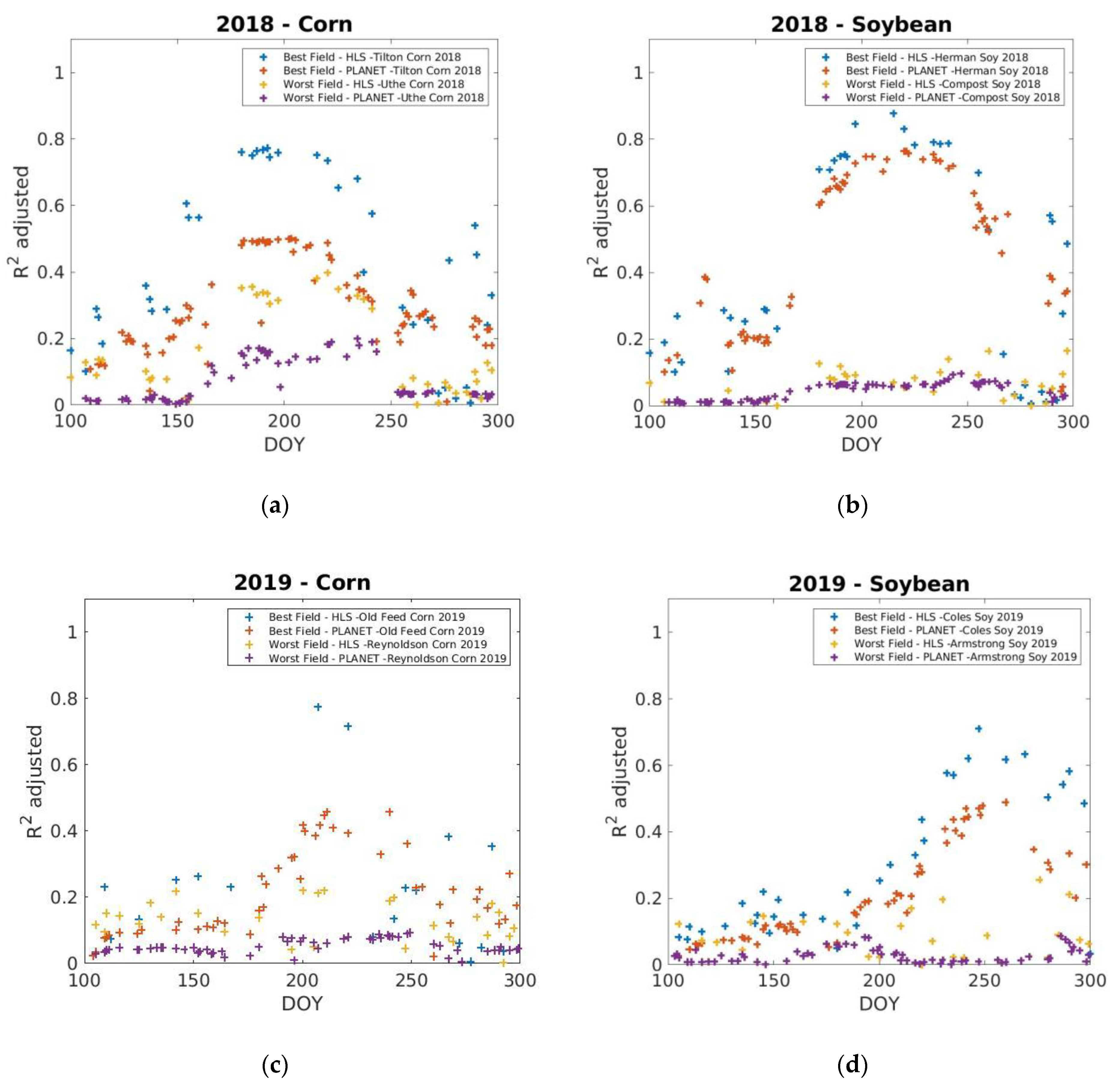
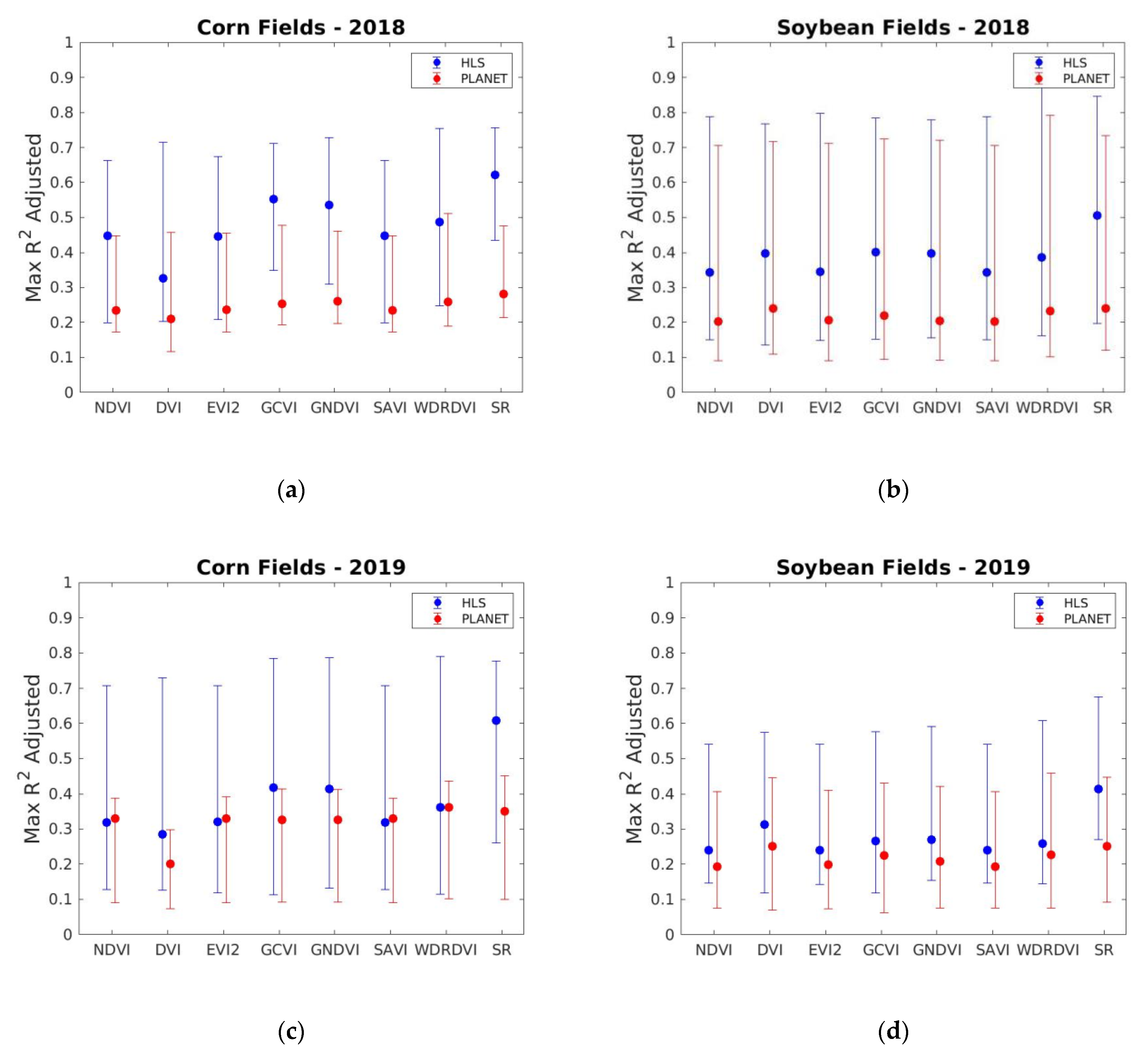
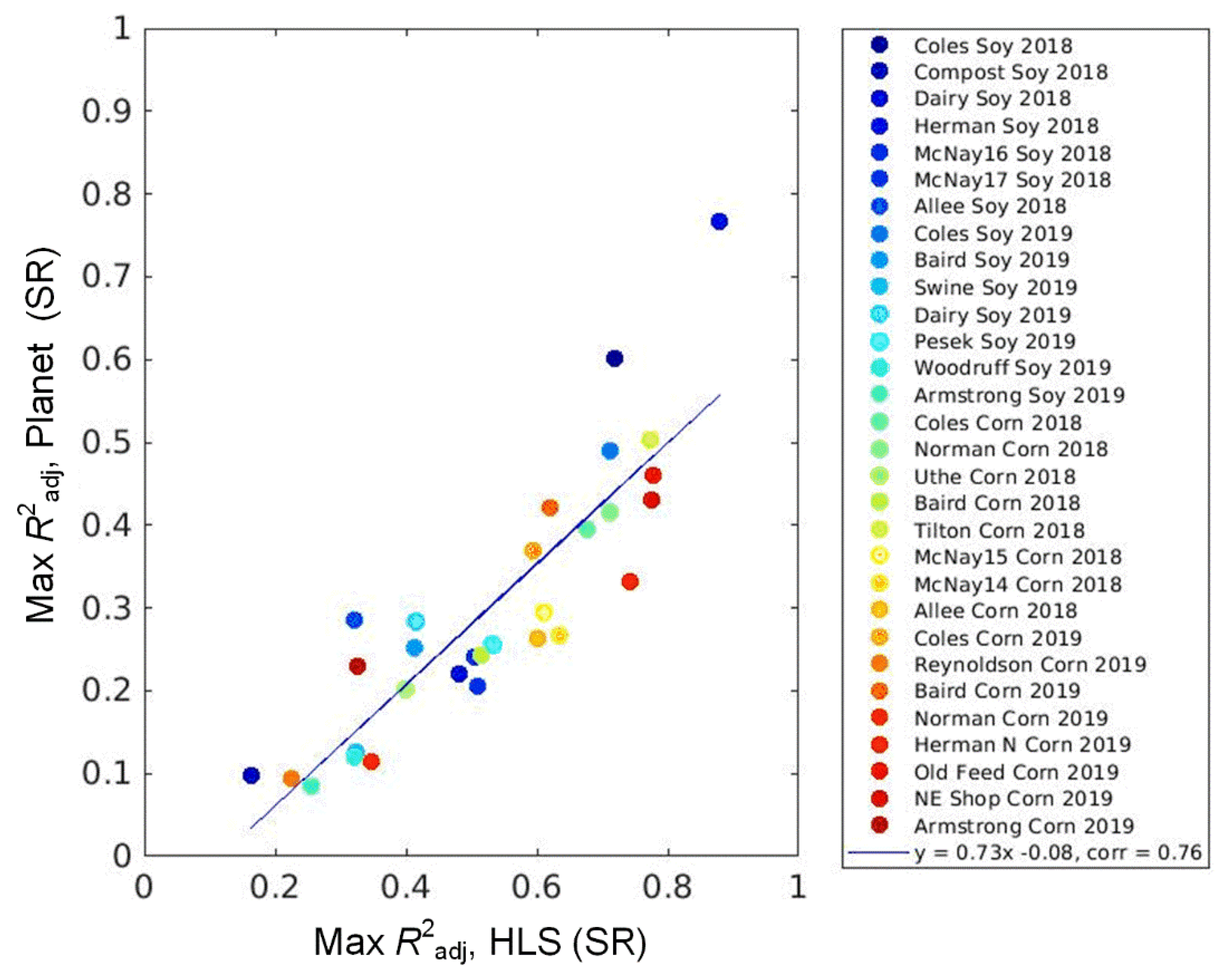
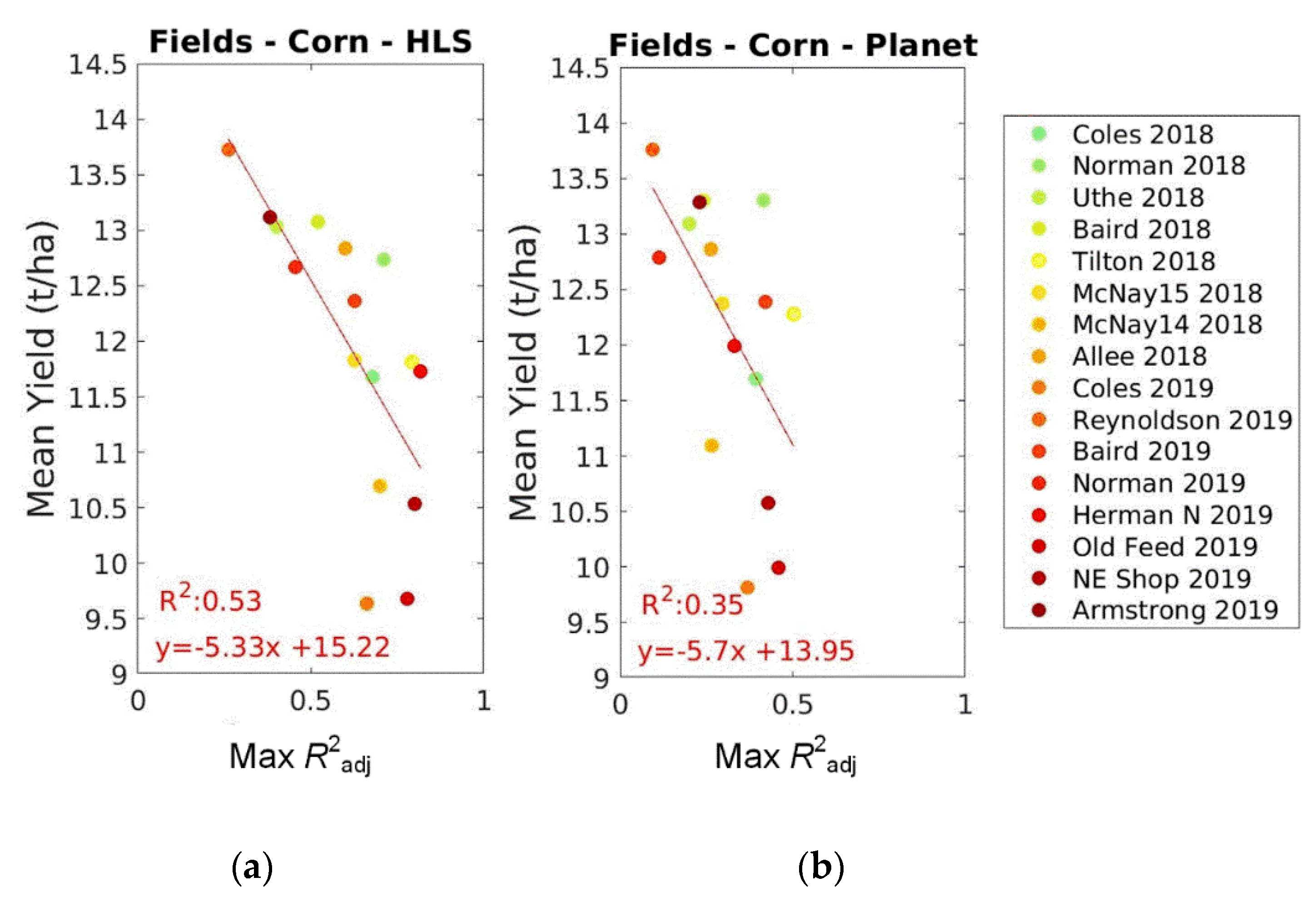
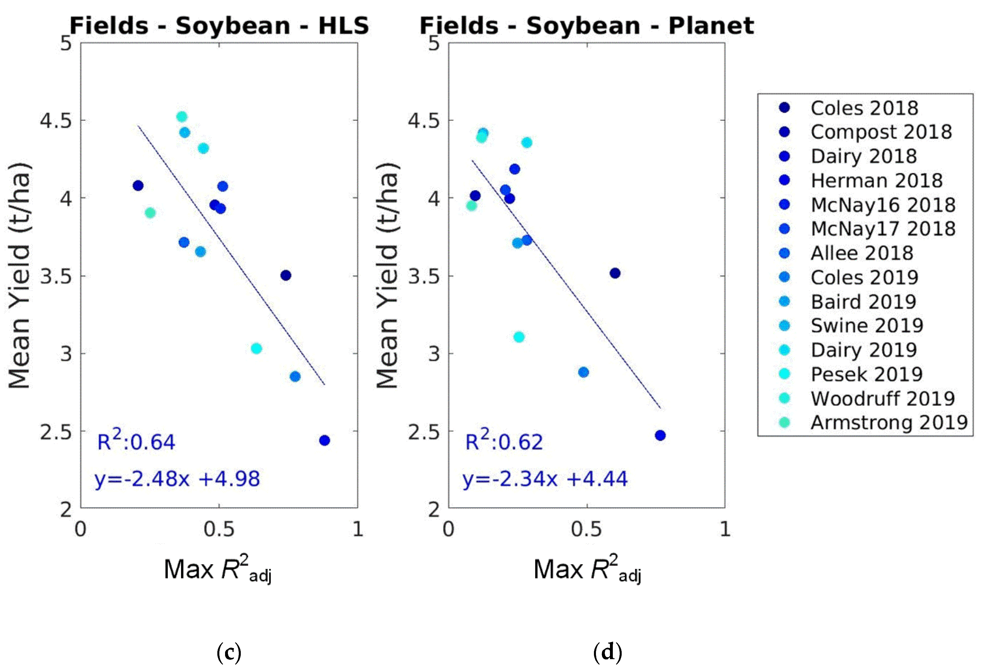
3.3. Analysis of Corn and Soybean Yield Varibility with Planet and HLS Data

Unlike with WV-3, Planet and HLS provided a dense time series of multi-spectral images, which allowed the determination of R² optimized timing to correlate satellite-derived features with yields. Figure 9 shows examples of how R² changes with time for some of the corn and the soybean fields in 2018 and 2019. Results show that, for some fields, a clear peak was visible, and R² reached values up to 0.8, suggesting possibility to explain up to 80% of within-field yield variability, whereas, for other fields, the maximum seasonal R² was around 0.1–0.2, suggesting that multi-spectral HLS and Planet data failed to explain within-field yield variability.

Table 3. Day of year (DOY) for which the maximal R² was achieved when correlating satellite-derived SR against crop yields along with crops harvesting dates. HLS: Harmonized Landsat Sentinel-2.

Crop	Year	Harvest	HLS	Planet
Corn	2018	298 ± 8	195 ± 19	206 ± 22
Corn	2019	307 ± 12	206 ± 22	216 ± 26
Soybean	2018	297 ± 6	209 ± 20	221 ± 16
Soybean	2019	292 ± 11	227 ± 24	223 ± 22

shows DOY values for which maximal was R² achieved and its correspondence to the harvesting date. The maximal correlation was observed 90–100 days (3 months) before corn harvest and 70–80 days (2–2.5 months) before soybean harvest.

Overall, the variable performance in terms of R² was observed when using SR and VI satellite-derived features to explain corn and soybean yield variability (Figure 10). Best results for HLS and Planet were obtained using a linear model incorporating all spectral bands. This outperformed models utilizing vegetation indices. For HLS, the SR-based models gave R² = 0.62 ± 0.16 (RMSE = 0.95 ± 0.34 t/ha) and 0.50 ± 0.20 (RMSE = 0.39 ± 0.15 t/ha) for corn and soybean, respectively. Average and standard deviation values of R² and RMSE were calculated for all corn and soybean fields in 2018 and 2019. The best VIs models were those based on green and NIR spectral bands such as the WV-3 case. Both GCVI and GNDVI gave R² = 0.48 ± 0.20 (RMSE = 1.07 ± 0.47 t/ha) and 0.35 ± 0.22 (RMSE = 0.46 ± 0.17 t/ha) for corn and soybean, respectively. Similar results were achieved for Planet, though the difference between the SR-based model and the best VIs models was less prominent, 0.32 ± 0.12 (RMSE = 1.92 ± 0.56 t/ha) compared to 0.29 ± 0.13 (RMSE = 1.98 ± 0.57 t/ha) for corn and 0.29 ± 0.20 (RMSE = 0.79 ± 0.41 t/ha) compared to 0.30 ± 0.23 (RMSE = 0.80 ± 0.41 t/ha) for soybean. Overall, R² values for corn were higher than those for soybean. Addition of SWIR bands to blue, green, red, and NIR bands in the HLS-based models slightly improved R² performance from 0.59 ± 0.17 and 0.62 ± 0.16 for corn and from 0.47 ± 0.20 and 0.50 ± 0.20 for soybean.

R² values obtained for HLS were higher than those obtained for Planet because of different scales employed (3 m vs. 30 m, or an order of 10 × 10 = 100). Averaging 3 m yield values to the 30 m HLS resolution reduces the variance of yield (Figure 5) that could be explained with satellite data, therefore increasing the coefficient of determination. Overall, a strong correlation between HLS- and Planet-based models was observed (Figure 11), suggesting consistency of results achieved with HLS and Planet data. In other words, the same set of fields gave higher or lower R² values for both Planet and HLS.

We found a strong correlation between R² and field-averaged corn and soybean yields (Figure 12). As the yield values increased, the performance of HLS- and Planet-based models to explain within-field yield variability decreased. Such dependence was stronger for soybean fields than for corn. R² values were less than 0.5 for corn and soybean fields with yields larger than 12.5 t/ha and 3.5 t/ha, respectively. These results show limitations in using multi-spectral satellite imagery in explaining within-field corn and soybean yield variability, especially for fields with large yield values. We did not find strong correlations between R² and yield variance or CV.

4. Discussion and Conclusions

This study aimed at investigating the efficiency of multi-spectral satellite imagery at various spatial and temporal resolutions to explain within-field yield variability for corn and soybean crops. First, we explored the effect of spatial resolution on yield variability. We found that reducing spatial resolution from 3 m to 30 m reduced yield variance at field scale with relative efficiency (Equation 1) decreasing from 1.0 to 0.6 (Figure 5), therefore decreasing capabilities of capturing within-field yields with moderate spatial resolution sensors. At the same time, the variance of yields inside 10, 20, or 30 m pixels increased up to 20% (Figure 6). These results are consistent with previous recommendations established within the VALERI protocol [18] to validate coarse and moderate resolution remote sensing products and have implications on collecting ground-based crop yields, for example, through crop cuts [14,15]. When validating coarse (100 m–1 km) and moderate (10–30 m) resolution crop yield maps, one must ensure that variability inside the pixel is captured through multiple (10–15) point-based samples.

In order to detect the optimal timing of correlating satellite-derived features with corn and soybean yields, a high temporal resolution of satellite data was required. This was achieved through the use of near-daily Planet data and a combination of 3–5 day revisit cycles of Sentinel-2 and Landsat 8 combined [33]. The maximal correlations for corn and soybean were obtained at 3 and 2–2.5 months, respectively, which is consistent with previous studies utilizing coarse resolution MODIS data and county-level yields [36]. We observed a very variable performance of these datasets to explain within-field yield variability: coefficient of determination R² (Equations (3) and (4)) varied from 0.21 to 0.88 (average 0.56 ± 0.19) for 30 m HLS and from 0.09 to 0.77 (0.30 ± 0.16) for 3 m Planet. Obtained R² values were higher for HLS than Planet because of various scales employed; averaging 3 m yields to 30 m reduced within-field yield variance (Figure 5), therefore potentially benefiting moderate resolution at the expense of details lost. R² values were also higher for corn than soybean, which is consistent with previous works utilizing remote sensing data and usually showing better performance for corn [7,36,37]. The maximal correlation between satellite-derived features and yields was observed 2–3 months before the harvest, therefore potentially enabling yield forecasts at field scale end of July to mid-August. We also found that performance of the satellite-derived models was better for corn and soybean fields with lower average yields: as the yields increase, R² values decrease. It means that multi-spectral data saturate over high yields and cannot capture yield variability. Other variables at such 3 to 30 m scale, such as soil moisture and evapotranspiration (ET) [38,39,40], irrigation vs. rainfed, should be considered, as previous studies showed that field-scale yield variability for corn and soybean in the US is mainly attributed to soil differences in the field and the water holding capacity [41].

In terms of spectral bands, green (~0.560 μm) and NIR (~0.865 μm) were the most important for Planet and HLS to explain corn and soybean within-field yield variability. We did not consider red-edge from Sentinel-2, since it is not available in Landsat 8. When analyzing WV-3 data, red-edge (0.726 μm) showed to be the most important in explaining yield variability. Overall, SR-based models outperformed VI-based models highlighting the importance of incorporating SR values directly into the yield models [9]. VIs based on NIR and red-edge or green spectral bands performed better than those based on NIR and red, as the former previously showed a better correspondence to corn and soybean productivity [42].

The further research should focus on the within-field water-stress indicators that can be retrieved using the fusion of satellite data and corresponding models and active remote sensing sensors such as synthetic aperture radar (SAR) and LIDAR.

References

1. Whitcraft, A.K.; Becker-Reshef, I.; Justice, C.O.; Gifford, L.; Kavvada, A.; Jarvis, I. No pixel left behind: Toward integrating Earth Observations for agriculture into the United Nations Sustainable Development Goals framework. Remote Sens. Environ. 2019, 235, 111470. [Google Scholar] [CrossRef]
2. Becker-Reshef, I.; Barker, B.; Humber, M.; Puricelli, E.; Sanchez, A.; Sahajpal, R.; McGaughey, K.; Justice, C.; Baruth, B.; Wu, B.; et al. The GEOGLAM crop monitor for AMIS: Assessing crop conditions in the context of global markets. Glob. Food Secur. 2019, 23, 173–181. [Google Scholar] [CrossRef]
3. Birrell, S.J.; Sudduth, K.A.; Borgelt, S.C. Comparison of sensors and techniques for crop yield mapping. Comput. Electron. Agric. 1996, 14, 215–233. [Google Scholar] [CrossRef]
4. Lobell, D.B. The use of satellite data for crop yield gap analysis. Field Crop. Res. 2013, 143, 56–64. [Google Scholar] [CrossRef] [Green Version]
5. Van Ittersum, M.K.; Cassman, K.G.; Grassini, P.; Wolf, J.; Tittonell, P.; Hochman, Z. Yield gap analysis with local to global relevance—A review. Field Crop. Res. 2013, 143, 4–17. [Google Scholar] [CrossRef] [Green Version]
6. Bokusheva, R.; Kogan, F.; Vitkovskaya, I.; Conradt, S.; Batyrbayeva, M. Satellite-based vegetation health indices as a criteria for insuring against drought-related yield losses. Agric. For. Meteorol. 2016, 220, 200–206. [Google Scholar] [CrossRef] [Green Version]
7. Johnson, D.M. A comprehensive assessment of the correlations between field crop yields and commonly used MODIS products. Int. J. Appl. Earth Obs. Geoinf. 2016, 52, 65–81. [Google Scholar] [CrossRef] [Green Version]
8. Franch, B.; Vermote, E.F.; Skakun, S.; Roger, J.-C.; Becker-Reshef, I.; Murphy, E.; Justice, C. Remote sensing based yield monitoring: Application to winter wheat in United States and Ukraine. Int. J. Appl. Earth Obs. Geoinf. 2019, 76, 112–127. [Google Scholar] [CrossRef]
9. Skakun, S.; Vermote, E.; Franch, B.; Roger, J.-C.; Kussul, N.; Ju, J.; Masek, J. Winter Wheat Yield Assessment from Landsat 8 and Sentinel-2 Data: Incorporating Surface Reflectance, Through Phenological Fitting, into Regression Yield Models. Remote Sens. 2019, 11, 1768. [Google Scholar] [CrossRef] [Green Version]
10. Kussul, N.; Lavreniuk, M.; Kolotii, A.; Skakun, S.; Rakoid, O.; Shumilo, L. A workflow for Sustainable Development Goals indicators assessment based on high-resolution satellite data. Int. J. Digit. Earth 2020, 13, 309–321. [Google Scholar] [CrossRef]
11. Roy, D.P.; Wulder, M.A.; Loveland, T.R.; Woodcock, C.E.; Allen, R.G.; Anderson, M.C.; Helder, D.; Irons, J.R.; Johnson, D.M.; Kennedy, R.; et al. Landsat-8: Science and product vision for terrestrial global change research. Remote Sens. Environ. 2014, 145, 154–172. [Google Scholar] [CrossRef] [Green Version]
12. Drusch, M.; Del Bello, U.; Carlier, S.; Colin, O.; Fernandez, V.; Gascon, F.; Hoersch, B.; Isola, C.; Laberinti, P.; Martimort, P.; et al. Sentinel-2: ESA’s optical high-resolution mission for GMES operational services. Remote Sens. Environ. 2012, 120, 25–36. [Google Scholar] [CrossRef]
13. Yang, C.; Everitt, J.H.; Du, Q.; Luo, B.; Chanussot, J. Using high-resolution airborne and satellite imagery to assess crop growth and yield variability for precision agriculture. Proc. IEEE 2013, 101, 582–592. [Google Scholar] [CrossRef]
14. Jain, M.; Srivastava, A.K.; Joon, R.K.; McDonald, A.; Royal, K.; Lisaius, M.C.; Lobell, D.B. Mapping smallholder wheat yields and sowing dates using micro-satellite data. Remote Sens. 2016, 8, 860. [Google Scholar] [CrossRef] [Green Version]
15. Sahajpal, R.; Becker-Reshef, I.; Coutu, S. Optimizing Crop Cut Collection for Determining Field-Scale Yields in an Insurance Context. Workshop Fragile Earth Data Sci. Sustain. Planet 2020. [Google Scholar] [CrossRef]
16. Gallego, F.J. Remote sensing and land cover area estimation. Int. J. Remote Sens. 2004, 25, 3019–3047. [Google Scholar] [CrossRef]
17. Olofsson, P.; Foody, G.M.; Herold, M.; Stehman, S.V.; Woodcock, C.E.; Wulder, M.A. Good practices for estimating area and assessing accuracy of land change. Remote Sens. Environ. 2014, 148, 42–57. [Google Scholar] [CrossRef]
18. Morisette, J.T.; Baret, F.; Privette, J.L.; Myneni, R.B.; Nickeson, J.E.; Garrigues, S.; Shabanov, N.V.; Weiss, M.; Fernandes, R.A.; Leblanc, S.G.; et al. Validation of global moderate-resolution LAI products: A framework proposed within the CEOS land product validation subgroup. IEEE Trans. Geosci. Remote Sens. 2006, 44, 1804–1817. [Google Scholar] [CrossRef] [Green Version]
19. Chang, J.; Clay, D.E.; Dalsted, K.; Clay, S.; O’Neill, M. Corn (Zea mays L.) yield prediction using multispectral and multidate reflectance. Agron. J. 2003, 95, 1447–1453. [Google Scholar] [CrossRef]
20. Dobermann, A.; Ping, J.L. Geostatistical integration of yield monitor data and remote sensing improves yield maps. Agron. J. 2004, 96, 285–297. [Google Scholar] [CrossRef]
21. Yang, C.; Everitt, J.H.; Bradford, J.M. Evaluating high resolution SPOT 5 satellite imagery to estimate crop yield. Precis. Agric. 2009, 10, 292–303. [Google Scholar] [CrossRef]
22. Hamada, Y.; Ssegane, H.; Negri, M.C. Mapping intra-field yield variation using high resolution satellite imagery to integrate bioenergy and environmental stewardship in an agricultural watershed. Remote Sens. 2015, 7, 9753–9768. [Google Scholar] [CrossRef] [Green Version]
23. Peralta, N.R.; Assefa, Y.; Du, J.; Barden, C.J.; Ciampitti, I.A. Mid-season high-resolution satellite imagery for forecasting site-specific corn yield. Remote Sens. 2016, 8, 848. [Google Scholar] [CrossRef] [Green Version]
24. Mulla, D.J. Twenty five years of remote sensing in precision agriculture: Key advances and remaining knowledge gaps. Biosyst. Eng. 2013, 114, 358–371. [Google Scholar] [CrossRef]
25. Kharel, T.P.; Swink, S.N.; Maresma, A.; Youngerman, C.; Kharel, D.; Czymmek, K.J.; Ketterings, Q.M. Yield monitor data cleaning is essential for accurate corn grain and silage yield determination. Agron. J. 2019, 111, 509–516. [Google Scholar] [CrossRef]
26. Sun, W.; Whelan, B.; McBratney, A.B.; Minasny, B. An integrated framework for software to provide yield data cleaning and estimation of an opportunity index for site-specific crop management. Precis. Agric. 2013, 14, 376–391. [Google Scholar] [CrossRef]
27. Neigh, C.S.; Masek, J.G.; Nickeson, J.E. High-resolution satellite data open for government research. Eos Trans. Am. Geophys. Union 2013, 94, 121–123. [Google Scholar] [CrossRef] [Green Version]
28. Vermote, E.; Justice, C.; Claverie, M.; Franch, B. Preliminary analysis of the performance of the Landsat 8/OLI land surface reflectance product. Remote Sens. Environ. 2016, 185, 46–56. [Google Scholar] [CrossRef] [PubMed]
29. Doxani, G.; Vermote, E.; Roger, J.-C.; Gascon, F.; Adriaensen, S.; Frantz, D.; Hagolle, O.; Hollstein, A.; Kirches, G.; Li, F.; et al. Atmospheric correction inter-comparison exercise. Remote Sens. 2018, 10, 352. [Google Scholar] [CrossRef] [PubMed] [Green Version]
30. NASA. “Private Sector Small Constellation Satellite Data Product Pilot” Program. Available online: https://earthdata.nasa.gov/esds/small-satellite-data-buy-program/csdap-pilot-evaluation (accessed on 25 February 2021).
31. Planet Team. Planet Application Program Interface: In Space for Life on Earth. San Francisco, CA, USA. 2017. Available online: https://api.planet.com (accessed on 25 February 2021).
32. Claverie, M.; Ju, J.; Masek, J.G.; Dungan, J.L.; Vermote, E.F.; Roger, J.-C.; Skakun, S.; Justice, C. The Harmonized Landsat and Sentinel-2 surface reflectance data set. Remote Sens. Environ. 2018, 219, 145–161. [Google Scholar] [CrossRef]
33. Li, J.; Roy, D.P. A global analysis of Sentinel-2A, Sentinel-2B and Landsat-8 data revisit intervals and implications for terrestrial monitoring. Remote Sens. 2017, 9, 902. [Google Scholar]
34. Gallego, F.J.; Kussul, N.; Skakun, S.; Kravchenko, O.; Shelestov, A.; Kussul, O. Efficiency assessment of using satellite data for crop area estimation in Ukraine. Int. J. Appl. Earth Obs. Geoinf. 2014, 29, 22–30. [Google Scholar] [CrossRef]
35. Strobl, C.; Boulesteix, A.L.; Kneib, T.; Augustin, T.; Zeileis, A. Conditional variable importance for random forests. BMC Bioinform. 2008, 9, 307. [Google Scholar] [CrossRef] [PubMed] [Green Version]
36. Johnson, D.M. An assessment of pre-and within-season remotely sensed variables for forecasting corn and soybean yields in the United States. Remote Sens. Environ. 2014, 141, 116–128. [Google Scholar] [CrossRef]
37. Gao, F.; Anderson, M.; Daughtry, C.; Johnson, D. Assessing the variability of corn and soybean yields in central Iowa using high spatiotemporal resolution multi-satellite imagery. Remote Sens. 2018, 10, 1489. [Google Scholar] [CrossRef] [Green Version]
38. Mladenova, I.E.; Bolten, J.D.; Crow, W.T.; Anderson, M.C.; Hain, C.R.; Johnson, D.M.; Mueller, R. Intercomparison of soil moisture, evaporative stress, and vegetation indices for estimating corn and soybean yields over the US. IEEE J. Sel. Top. Appl. Earth Obs. Remote Sens. 2017, 10, 1328–1343. [Google Scholar] [CrossRef]
39. Yang, Y.; Anderson, M.C.; Gao, F.; Wardlow, B.; Hain, C.R.; Otkin, J.A.; Alfieri, J.; Yang, Y.; Sun, L.; Dulaney, W. Field-scale mapping of evaporative stress indicators of crop yield: An application over Mead, NE, USA. Remote Sens. Environ. 2018, 210, 387–402. [Google Scholar] [CrossRef]
40. Anderson, M.C.; Yang, Y.; Xue, J.; Knipper, K.R.; Yang, Y.; Gao, F.; Hain, C.R.; Kustas, W.P.; Cawse-Nicholson, K.; Hulley, G.; et al. Interoperability of ECOSTRESS and Landsat for mapping evapotranspiration time series at sub-field scales. Remote Sens. Environ. 2021, 252, 112189. [Google Scholar] [CrossRef]
41. Hatfield, J.L.; Aflakpui, G. Spatial patterns of water and nitrogen response within corn production fields. In Agricultural Science; Aflakpui, G., Ed.; InTech: Rijeka, Croatia, 2012; pp. 73–96. [Google Scholar]
42. Peng, Y.; Gitelson, A.A. Remote estimation of gross primary productivity in soybean and maize based on total crop chlorophyll content. Remote Sens. Environ. 2012, 117, 440–448. [Google Scholar] [CrossRef]
Figure 1. Distribution of corn and soybean fields in Iowa, USA.
Remotesensing 13 00872 g001
Figure 2. Per-field average yield values along with median (solid line) and 10 and 90 percentiles (dashed lines) and planting (bottom circles) and harvest (top circles) dates for corn (a) and soybean (b) fields represented as day of year (DOY).
Remotesensing 13 00872 g002
Figure 3. Example of yield distribution over the Coles fields in 2019 as acquired by combine harvester.
Remotesensing 13 00872 g003
Figure 4. Example of WorldView-3 (WV-3) images acquired over the Coles corn field on 2 July 2018. True color composite red-green-blue (a); false color composite near infrared (NIR)-red-green (b); corn yields (c). © 2021 DigitalGlobe, Inc., a Maxar company, NextView License.
Remotesensing 13 00872 g004
Figure 5. Dependence of the relative efficiency, the metric showing how well one can capture yield variability, on spatial resolution. These results were obtained by simulating yields from the harvester machinery at various spatial resolutions.
Remotesensing 13 00872 g005
Figure 6. Histogram of coefficient of variation of yields inside a moderate spatial resolution pixel (10, 20, and 30 m).
Remotesensing 13 00872 g006
Figure 7. Dependencies between corn yields and NDVI, WDRVI, GCVI, and CIre as derived from the WV-3 imagery acquired on 21 July 2018, 66 days after the planting date. Number of samples is 17,802.
Remotesensing 13 00872 g007
Figure 8. Relative importance of WV-3 spectral bands when correlating them with corn yields. WV-3 was acquired on 21 July 2018. Shown also is R2 for the linear model between SR values and corn yields.
Remotesensing 13 00872 g008
Figure 9. Coefficient of determination R adj 2 as a function of the day of year for the best and the worst fields using HLS- and Planet-derived SR values to correlate with yields: (a) corn in 2018; (b) soybean in 2018; (c) corn in 2019; (d) soybean in 2019.
Remotesensing 13 00872 g009
Figure 10. Median along with 10th and 90th percentile values of the maximum of coefficient of determination R adj 2 for various HLS- and Planet-derived features: (a)–(c) for corn and (b)–(d) for soybean.
Remotesensing 13 00872 g010
Figure 11. Comparison of R2 for best models between corn and soybean yields and SR values obtained with HLS and Planet data.
Remotesensing 13 00872 g011
Figure 12. Dependence of the coefficient of determination R2 for the best HLS- and Planet-based models on field yield: (a)–(b) for corn and (c)–(d) for soybean.
Remotesensing 13 00872 g012aRemotesensing 13 00872 g012b