Radar HRRP Target Recognition Based on Dynamic Learning with Limited Training Data

Abstract

For high-resolution range profile (HRRP)-based radar automatic target recognition (RATR), adequate training data are required to characterize a target signature effectively and get good recognition performance. However, collecting enough training data involving HRRP samples from each target orientation is hard. To tackle the HRRP-based RATR task with limited training data, a novel dynamic learning strategy is proposed based on the single-hidden layer feedforward network (SLFN) with an assistant classifier. In the offline training phase, the training data are used for pretraining the SLFN using a reduced kernel extreme learning machine (RKELM). In the online classification phase, the collected test data are first labeled by fusing the recognition results of the current SLFN and assistant classifier. Then the test samples with reliable pseudolabels are used as additional training data to update the parameters of SLFN with the online sequential RKELM (OS-RKELM). Moreover, to improve the accuracy of label estimation for test data, a novel semi-supervised learning method named constraint propagation-based label propagation (CPLP) was developed as an assistant classifier. The proposed method dynamically accumulates knowledge from training and test data through online learning, thereby reinforcing performance of the RATR system with limited training data. Experiments conducted on the simulated HRRP data from 10 civilian vehicles and real HRRP data from three military vehicles demonstrated the effectiveness of the proposed method when the training data are limited.

1. Introduction

A high-resolution range profile (HRRP) provides the geometrical shape and structural characteristics of a target along the radar line-of-sight (LOS). Compared to synthetic aperture radar (SAR) [1] and inverse SAR images, it is easier to get and store. Therefore, HRRP has been widely used for radar automatic target recognition (RATR) systems.

A typical RATR system comprises the feature extraction followed by a powerful classifier. Various target features from HRRP have been developed over the years, such as spectral features [2,3], scattering center features [4,5], statistical features [6,7,8], high-level features learned from deep networks [9,10] and so on. Typical classifiers applied to HRRP-based RATR include the template matching method (TMM) [4,5], Bayes’ classifier [6,7,8], the hidden Markov model (HMM) [11], etc.

To get good recognition performance, the methods above require complete training data which are an effective representation of the target’s signature. However, acquisition of enough target HRRPs is difficult in many real applications. The main reasons are these: First, the targets of interest may be noncooperative and their echoes can be hard to collect. Second, due to the aspect-sensitivity of the target HRRP, the complete training data should involve HRRP samples of all possible orientations, which is unrealistic in practice. When the available training data are limited, the RATR system will exhibit unsatisfactory performance even though the extracted feature and classifier used are good enough. Therefore, developing an HRRP-based RATR method with limited training data is important.

Some studies have reported to deal with the RATR task with limited training data. The support vector machine (SVM) [12] has been widely used for HRRP-based target recognition [13], since it can get the smallest generalization error and is suitable for small sample learning. However, the SVM does not consider the overall characteristics of the target feature, which makes it sensitive to missing data. In [14], the dictionary learning (DL) method, i.e., the K-SVD algorithm, was employed to classify HRRPs of a target when training data were limited, for it shares the latent information among samples. Motivated by [14], reference [15] proposed a robust DL method which overcomes the uncertainty of sparse representations and is robust to the amplitude variations of adjacent HRRPs. It achieves good recognition performance with limited training data. In [16], a factor analysis model was proposed based on multitask learning (MTL), in which the relevant information among HRRP samples with different target aspects is employed, and the aspect-dependent parameters are obtained collectively. This method can reduce the number of HRRP samples required in each target aspect-frame. However, the MTL and robust DL models still require dozens of HRRP samples in each target aspect-frame to estimate parameters, which may not be realized in practice. In [17], the discriminant deep autoencoder (DDAE) was proposed to extract high-level features of HRRPs and train HRRP samples globally, which enhances the recognition performance with little training data compared to most methods.

The above methods above are supervised learning approaches whose classifiers stay unchanged during the classification process. They only take advantage of the offline training data and ignore the useful information from new samples collected during the classification process. Considering this, Yver [18] proposed a dynamic learning strategy which updates the classifier using test samples. This strategy requires the RATR system to accumulate knowledge dynamically, and exploit the knowledge to facilitate future learning and classification in the update process. Four online learning approaches were presented, including online self-training label-propagation (LP) [19], self-training LASVM [20], a combination of LP and LASVM, and online TSVM. Nevertheless, these methods come with several drawbacks. The self-training method teaches itself using the learned knowledge, so it cannot reduce the bias caused by the limited training data [21]. LASVM gets the approximate classification model in one-by-one mode but not in chunk-by-chunk mode, so its computation is time-consuming. In [22], an updating convolutional neural network (CNN) was proposed for use with SAR images. The initial CNN model trained by the seed images was updated using the test images whose pseudolabels were assigned with the SVM. This method exhibited good recognition performance on the MSTAR dataset. However, it must store all the test data during the update process, which burdens the memory resources.

Single-hidden layer feedforward neural networks (SLFNs) have been widely used in pattern recognition (PR). The reduced kernel extreme learning machine (RKELM) [23] is a kernel-based learning technique for SLFN in which the mapping samples are selected from the training dataset and the output weights are analytically determined. In theory, it can provide good generalization performance at high learning speed. The online sequential RKELM (OS-RKELM) [24] is a fast online learning algorithm that can process data in chunk-by-chunk mode and discard data after they have been learned. Hence, it achieves savings in terms of both processing time and memory resources. However, the OS-RKELM is a supervised learning method that requires the online received data to be labeled, and it cannot be applied directly to the HRRP-based RATR task.

In this paper, a novel dynamic learning method based on the SLFN with an assistant classifier is proposed to enhance the performance of HRRP-based RATR with limited training data. In the offline training stage, the initial SLFN model is trained with the RKELM algorithm using the labeled training data. In the classification stage, two steps, i.e., the pseudolabel assignment and SLFN parameter update steps, are iterated. Once a certain number of test samples are collected, their pseudolabels are assigned. Then, the test samples with reliable pseudolabels are considered as additional training data to update the SLFN parameters by the OS-RKELM. Particularly, to improve the accuracy of label estimation for test data, a novel semi-supervised learning method named constraint propagation-based label propagation (CPLP) was developed as an assistant classifier, in which the offline training samples are viewed as labeled data and the newly collected test samples as unlabeled data. The pseudolabel of each test sample is assigned by fusing the classification results of CPLP and the SLFN. Through the dynamic learning strategy, the HRRP-based RATR system dynamically accumulates knowledge from both offline training data and online test data, thereby reinforcing the performance of the RATR system.

Our contributions are summarized as follows:

• To deal with the HRRP-based RATR task with limited training data, a dynamic learning strategy is introduced based on the SLFN with an assistant classifier. The proposed method processes data chunk-by-chunk and discards the test data once they have been learned, so it requires less memory and processing time.
• A novel semi-supervised learning method named constraint propagation-based label propagation (CPLP) is proposed as an assistant classifier to improve the label estimation accuracy for test data.

In the experiments, the effectiveness of the proposed method was demonstrated on two datasets, i.e., simulated data of 10 civilian vehicles and measured data of three military vehicles. In this paper, the superiority of the CPLP algorithm is verified first. Then, the recognition performance of the proposed SLFN with the CPLP algorithm is presented along with the update process. By leaning information from the test data, a performance improvement was achieved when training data were limited. Next, the comparative experiments are shown, and the proposed method showed very competitive recognition performance with the state-of-the-art methods on the two datasets. Finally, the computational complexity is analyzed.

The remainder of this paper is organized as follows. Section 2 introduces the proposed algorithm in detail. Section 3 provides the experiment results on the simulated HRRP data of 10 civilian vehicles and the measured data of three military vehicles. Section 4 presents the conclusions.

2. Methodology

The framework of the proposed recognition method is shown in Figure 1. In the RKELM and OS-RKELM algorithms, the offline training data have to be stored in order to compute the kernel matrix in the online classification stage. Consequently, for the proposed CPLP algorithm, the offline training data are viewed as labeled samples, and the newly collected test data chunk (TDC) as unlabeled samples. The test samples with reliable pseudolabels are viewed as additional training data to update the SLFN model. Once a TDC is learned, it is discarded. The method continues to classify newly collected test data and exploit them to update the SLFN parameters. In this way, the knowledge of both the offline training data and the online test data can be accumulated in the SLFN model, and be used to facilitate future learning and classification alongside the update process.

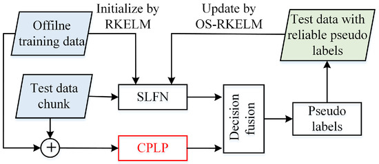
Figure 1. Framework of the proposed method.

For simplification purposes, some notation is as follows. ${\mathit{X}}_L=\left[{\mathit{x}}_1,\cdots ,{\mathit{x}}_{N_l}\right]$ is the offline training dataset (OTD) containing $N_l$ HRRP samples from C classes. ${\mathit{Y}}_L={\left[{\mathit{y}}_1,\cdots ,{\mathit{y}}_{N_l}\right]}^T\in R^{N_l\times C}$ is the label matrix with $y_{nc}=1$ if the label of sample ${\mathit{x}}_n$ is c; and $y_{nc}=0$ otherwise; $n=1,2,\cdots ,N_l$ and $c=1,2,\cdots ,C$. ${\mathit{X}}_m^U=\left[{\mathit{x}}_1^u,\cdots ,{\mathit{x}}_{N_u}^u\right]$ is the mth chunk of test HRRP data that is collected in the classification stage. The HRRP samples in ${\mathit{X}}_m^U$ are processed at a time during the update process.

In what follows, the SLFN classifier, CPLP algorithm, and decision fusion of SLFN and CPLP classifiers are introduced.

2.1. Single-Hidden Layer Feedforward Neural Network

In our proposed method, the SLFN has $N_l$ hidden nodes and C output nodes. The parameters of SLFN are initialized using the OTD ${\mathit{X}}_L$ by the RKELM. Let $\mathit{\beta }\in R^{N_l\times C}$ denote the output weights connecting the hidden layer and output layer; then its optimal value can be derived in closed from [23]

$$\begin{array}{c}\hfill {\mathit{\beta }}^{\left(0\right)}={\left(\frac{\mathit{I}}{\xi }+{\mathit{K}}_0^T{\mathit{K}}_0\right)}^{-1}{\mathit{K}}_0^T{\mathit{Y}}_L\end{array}$$

(1)

where ${\mathit{K}}_0$ is the kernel matrix of which the $(i,j)$th entry is computed by $K\left({\mathit{x}}_i,{\mathit{x}}_j\right)$, and the parameter $\xi$ is used to relax the overfitting issue of the SLFN model.

In the online classification stage, when the HRRP TDC ${\mathit{X}}_m^U$ is collected, the OS-RKELM updates ${\mathit{\beta }}^{\left(m\right)}$ as follows: [24]:

$$\begin{array}{c}\hfill {\mathit{G}}_m={\mathit{G}}_{m-1}-{\mathit{G}}_{m-1}{\mathit{K}}_m^T{\left(\mathit{I}+{\mathit{K}}_m{\mathit{G}}_{m-1}{\mathit{K}}_m^T\right)}^{-1}{\mathit{K}}_m{\mathit{G}}_{m-1}\end{array}$$

(2)

$$\begin{array}{c}\hfill {\mathit{\beta }}^{\left(m\right)}={\mathit{\beta }}^{\left(m-1\right)}+{\mathit{G}}_m{\mathit{K}}_m^T\left({\mathit{Y}}_m^s-{\mathit{K}}_m{\mathit{\beta }}^{\left(m-1\right)}\right)\end{array}$$

(3)

where ${\mathit{K}}_m=K\left({\mathit{X}}_m^U,{\mathit{X}}_L\right)$, ${\mathit{G}}_0={\left(\frac{\mathit{I}}{\xi }+{\mathit{K}}_0^T{\mathit{K}}_0\right)}^{-1}$, and ${\mathit{Y}}_m^s=\left[{\mathit{y}}_1^s,\cdots ,{\mathit{y}}_{N_u}^s\right]$ is the pseudolabel matrix of ${\mathit{X}}_m^U$.

Let ${\mathit{x}}_n^u$ be the nth test sample in ${\mathit{X}}_m^U$; its prediction is computed as [24]

$$\begin{array}{c}\hfill {\mathit{t}}_n^u=K\left({\mathit{x}}_n^u,{\mathit{X}}_L\right){\mathit{\beta }}^{\left(m-1\right)}\end{array}$$

(4)

Since the elements in ${\mathit{t}}_n^u$ are not probability values, we define the label probability vector ${\mathit{p}}_n^u=\left[p_1,p_2,\cdots ,p_C\right]$ of ${\mathit{x}}_n^u$ as

$$\begin{array}{c}\hfill p_c=\frac{exp\left(-a{∥{\mathit{t}}_n^u-{\mathit{t}}_c∥}_2^2\right)}{{\displaystyle \sum _{c=1}^C}exp\left(-a{∥{\mathit{t}}_n^u-{\mathit{t}}_c∥}_2^2\right)}\end{array}$$

(5)

where $p_c$ is the probability of ${\mathit{x}}_n^u$ belonging to the cth class, a is a constant greater than 0, ${\mathit{t}}_c$ is a C-dimensional row vector of which the cth element is 1 and the other elements are 0. Then

$$\begin{array}{c}\hfill {\mathit{P}}_m^U=\left[\begin{array}{c}{\mathit{p}}_1^u\\ ⋮\\ {\mathit{p}}_{N_u}^u\end{array}\right]\end{array}$$

(6)

is the label probability matrix of ${\mathit{X}}_m^U$ computed by the SLFN.

2.2. Constraint Propagation-Based Label Propagation

LP is a graph-based semi-supervised learning method which propagates the label information of labeled data to unlabeled data according to the intrinsic geometrical structure of the data. The graph construction method plays an important role in label estimation for unlabeled data.

According to the LP method, the label probability matrix ${\mathit{F}}_m^U$ of ${\mathit{X}}_m^U$ is estimated as [19]:

$$\begin{array}{c}\hfill {\mathit{F}}_m^U={\left(\mathit{I}-{\overline{\mathit{W}}}_{UU}\right)}^{-1}{\overline{\mathit{W}}}_{UL}{\mathit{Y}}_L\end{array}$$

(7)

where the nth row ${\mathit{f}}_n^u$ of ${\mathit{F}}_m^U$ is the probability vector whose element $f_{n,c}$ is the probability of ${\mathit{x}}_n^u$ belonging to the cth class. ${\overline{\mathit{W}}}_{UL}\in R^{N_u\times N_l}$ and ${\overline{\mathit{W}}}_{UU}\in R^{N_u\times N_u}$ are the normalized probabilistic transition matrices which measure similarities between unlabeled samples and labeled ones, and similarities between unlabeled samples, respectively. They are usually constructed in an unsupervised manner, such as using a k-nearest neighbor (k-NN) graph [25], which ignores the label information of labeled data. Considering this, we exploit the label information to encode the pairwise constraints [26,27] between labeled samples, and then construct ${\overline{\mathit{W}}}_{UL}$ by propagating the constraint information via the similarity. The motivation for this idea is twofold.

• If samples ${\mathit{x}}_k\in {\mathit{X}}_U$ and ${\mathit{x}}_i\in {\mathit{X}}_L$ are similar, and ${\mathit{x}}_j\in {\mathit{X}}_L$ has the same class as ${\mathit{x}}_i$, then ${\mathit{x}}_k$ tends to be similar to ${\mathit{x}}_j$.
• If samples ${\mathit{x}}_k,{\mathit{x}}_i\in {\mathit{X}}_U$ are similar, ${\mathit{x}}_k$ and ${\mathit{x}}_j\in {\mathit{X}}_L$ are similar, then both ${\mathit{x}}_i$ and ${\mathit{x}}_k$ are prone to having the same label as ${\mathit{x}}_j$.

The proposed CPLP algorithm consists of two steps. In the first step, the traditional unsupervised graph is constructed. Let ${\mathit{W}}_{UU}\in R^{N_u\times N_u}$ denote the affinity matrix characterizing the similarities among unlabeled data, and ${\mathit{W}}_{UL}\in R^{N_u\times N_l}$ denote the affinity matrix describing the similarities among labeled samples and unlabeled ones. Since HRRP is in high dimensional space, the k-reciprocal nearest neighbors (k-RNNs) [28,29] is adopted to compute the $\left(i,j\right)$th entry of ${\mathit{W}}_{UU}$ and ${\mathit{W}}_{UL}$ as follows.

$$\begin{array}{c}\hfill w_{ij}=\left\{\begin{array}{c}exp\left(-\frac{d{\left({\mathit{x}}_i,{\mathit{x}}_j\right)}^2}{{\sigma }^2}\right),{\mathit{x}}_i\in N\left({\mathit{x}}_j\right)\wedge {\mathit{x}}_j\in N\left({\mathit{x}}_i\right)\hfill \\ 0,otherwise\hfill \end{array}\right.\end{array}$$

(8)

where $N\left(\mathit{x}\right)$ is the k-NN sample set of $\mathit{x}$. For ${\mathit{W}}_{UU}$, we set ${\mathit{x}}_i,{\mathit{x}}_j\in {\mathit{X}}_m^U$. For ${\mathit{W}}_{UL}$, we define a dataset ${\mathit{D}}_k=\left[{\mathit{x}}_k,{\mathit{X}}_m^U\right]$, ${\mathit{x}}_k\in {\mathit{X}}_L$, and the entries in the kth column are computed by setting ${\mathit{x}}_i,{\mathit{x}}_j\in {\mathit{D}}_k$.

In the second step, we aim to propagate the constraint information of labeled data to unlabeled data via the affinity matrices ${\mathit{W}}_{UU}$ and ${\mathit{W}}_{UL}$.

First, To incorporate the known label information, the affinity matrix ${\mathit{W}}_{LL}\in R^{N_l\times N_l}$ among labeled data is constructed by imposing two kinds of pairwise constraints. If the samples ${\mathit{x}}_i$ and ${\mathit{x}}_j$ are from the same class, the must-link constraint is imposed. Otherwise, the cannot-link constraint is set. The entries of ${\mathit{W}}_{LL}$ are computed as [27]

$$\begin{array}{c}\hfill w_{ij}=\left\{\begin{array}{c}1,y_i=y_j\hfill \\ 0,y_i\ne y_j\hfill \end{array}\right.\end{array}$$

(9)

Then, the pairwise constraints are propagated to their nearest neighbors by an iterative process [27,30]. In the tth iteration, the ith row of ${\mathit{W}}_{UL}^{\left(t\right)}$ is computed as

$$\begin{array}{cc}\hfill {\mathit{W}}_{UL,i}^{\left(t\right)}& =\left(1-\alpha \right){\mathit{W}}_{UL,i}^{\left(0\right)}+\alpha \left(\sum _{j=1}^{N_l}{\mathit{M}}_{UL,ij}{\mathit{W}}_{LL,j}^{\left(t-1\right)}+\sum _{k=1}^{N_u}{\mathit{M}}_{UU,ik}{\mathit{W}}_{UL,k}^{\left(t-1\right)}\right)\hfill \end{array}$$

(10)

where $t=0,1,2,\cdots$ is the time stamp, ${\mathit{W}}_{UL}^{\left(0\right)}={\mathit{W}}_{UL}$, ${\mathit{W}}_{LL}^{\left(t\right)}={\mathit{W}}_{LL}$ is clamped, ${\mathit{W}}_{UL,i}^{\left(t\right)}$ denotes the ith row of ${\mathit{W}}_{UL}^{\left(t\right)}$, $\alpha \in \left[0,1\right)$ is the trade-off parameter, ${\mathit{M}}_{UL,ij}$ is the $\left(i,j\right)$th entry of ${\mathit{M}}_{UL}$, and ${\mathit{M}}_{UU,ik}$ is the $\left(i,k\right)$th entry of ${\mathit{M}}_{UU}$—the final two are calculated by (11) and (12), respectively.

$$\begin{array}{c}\hfill {\mathit{M}}_{UL,ij}={\mathit{W}}_{UL,ij}/\phantom{{\mathit{W}}_{UL,ij}\left(\sum _{j=1}^{N_l}{\mathit{W}}_{UL,ij}+\sum _{k=1}^{N_u}{\mathit{W}}_{UU,ik}\right)}\left(\sum _{j=1}^{N_l}{\mathit{W}}_{UL,ij}+\sum _{k=1}^{N_u}{\mathit{W}}_{UU,ik}\right)\end{array}$$

(11)

$$\begin{array}{c}\hfill {\mathit{M}}_{UU,ik}={\mathit{W}}_{UU,ik}/\phantom{{\mathit{W}}_{UU,ik}\left(\sum _{j=1}^{N_l}{\mathit{W}}_{UL,ij}+\sum _{k=1}^{N_u}{\mathit{W}}_{UU,ik}\right)}\left(\sum _{j=1}^{N_l}{\mathit{W}}_{UL,ij}+\sum _{k=1}^{N_u}{\mathit{W}}_{UU,ik}\right)\end{array}$$

(12)

The matrix form of Equation (10) is presented as

$$\begin{array}{c}\hfill {\mathit{W}}_{UL}^{\left(t\right)}=\left(1-\alpha \right){\mathit{W}}_{UL}^{\left(0\right)}+\alpha {\mathit{M}}_{UL}{\mathit{W}}_{LL}+\alpha {\mathit{M}}_{UU}{\mathit{W}}_{UL}^{\left(t-1\right)}\end{array}$$

(13)

When $t\to \infty$, ${\mathit{W}}_{UL}^{\left(t\right)}$ reaches a steady state ${\mathit{W}}_{UL}^{*}$ which is calculated as

$$\begin{array}{c}\hfill {\mathit{W}}_{UL}^{*}={\left(\mathit{I}-\alpha {\mathit{M}}_{UU}\right)}^{-1}\left[\left(1-\alpha \right){\mathit{W}}_{UL}+\alpha {\mathit{M}}_{UL}{\mathit{W}}_{LL}\right]\end{array}$$

(14)

Let ${\mathit{W}}_U=\left[{\mathit{W}}_{UL}^{*}{\mathit{W}}_{UU}\right]$; the normalized probabilistic transition matrices ${\overline{\mathit{W}}}_{UL}$ and ${\overline{\mathit{W}}}_{UU}$ are derived as

$$\begin{array}{c}\hfill {\overline{\mathit{W}}}_{UL,ij}={\mathit{W}}_{UL,ij}^{*}/\phantom{{\mathit{W}}_{UL,ij}^{*}\sum _{k=1}^{N_l+N_u}{\mathit{W}}_{U,ik}}\sum _{k=1}^{N_l+N_u}{\mathit{W}}_{U,ik}\end{array}$$

(15)

$$\begin{array}{c}\hfill {\overline{\mathit{W}}}_{UU,ij}={\mathit{W}}_{UU,ij}/\phantom{{\mathit{W}}_{UU,ij}\sum _{k=1}^{N_l+N_u}{\mathit{W}}_{U,ik}}\sum _{k=1}^{N_l+N_u}{\mathit{W}}_{U,ik}\end{array}$$

(16)

Then ${\mathit{F}}_m^U$ is estimated using (7).

The procedure of the proposed CPLP algorithm is depicted in Figure 2.

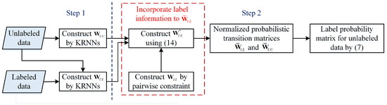
Figure 2. Flowchart of the proposed constraint propagation-based label propagation (CPLP) algorithm.

2.3. Decision Fusion

To improve the accuracy of label estimation for test data, we fuse the decisions of the SLFN and CPLP to get the final label probability of test samples. The fused probability vector ${\mathit{z}}_n^u$ of ${\mathit{x}}_n^u$ is obtained by

$$\begin{array}{c}\hfill {\mathit{z}}_n^u={\kappa }_n{\mathit{p}}_n^u+\left(1-{\kappa }_n\right){\mathit{f}}_n^u\end{array}$$

(17)

where ${\kappa }_n$ is a parameter controlling the relative contributions of classification results of the SLFN and CPLP algorithms for ${\mathit{x}}_n^u$. The more reliable the classification result of CPLP, the smaller the parameter $\kappa$. The classifier energy based evaluation [21] that thinks neighbor samples should have the same labels is used to compute $\kappa$ as follows.

Let $\mathbf{Y}=\left[{\mathit{X}}_L{\mathit{X}}_m^U\right]$, ${\mathit{E}}_1=\left[{\mathit{Y}}_L^T{\left({\mathit{P}}_m^U\right)}^T\right]$, ${\mathit{E}}_2=\left[{\mathit{Y}}_L^T{\left({\mathit{F}}_m^U\right)}^T\right]$, and $K{R}_n^u$ be the indices of KRNNs of $x_n^u$ in $\mathbf{Y}$. The energy-based evaluation of classifier for ${\mathit{x}}_n^u$ is defined as

$$\begin{array}{c}\hfill r_v\left(n\right)=\sum _{i=1}^{\left|K{R}_n^u\right|}{∥{\mathit{E}}_v\left(N_l+n\right)-{\mathit{E}}_v\left(K{R}_n^u\left(i\right)\right)∥}_2^2,v=1,2\end{array}$$

(18)

where ${\mathit{E}}_v\left(N_l+n\right)$ is the $\left(N_l+n\right)$th column of ${\mathit{E}}_v$, and $\left|K{R}_n^u\right|$ is the number of samples in $K{R}_n^u$. Then ${\kappa }_n$ is computed as

$$\begin{array}{c}\hfill {\kappa }_n=r_2\left(n\right)/\phantom{r_2\left(n\right)\left(r_1\left(n\right)+r_2\left(n\right)\right)}\left(r_1\left(n\right)+r_2\left(n\right)\right)\end{array}$$

(19)

Then the pseudolabel of ${\mathit{x}}_n^u$ is assigned as $c^{*}=\underset{c}{argmax}{\mathit{z}}_n^u$, and the corresponding label probability is $max\left({\mathit{z}}_n^u\right)$. We select the test samples in the top one percent (p) of label probability as additional training data to update the SLFN parameters.

3. Experiment Results and Analysis

In this section, the effectiveness of the proposed HRRP-based RATR method is demonstrated by experiments that used limited training data. Two datasets, the simulated HRRP dataset of 10 civilian vehicles and the measured HRRP dataset of three military vehicles, were tested. First, the superiority of the proposed CPLP method is verified. Then, the recognition performance of the proposed SLFN with CPLP method is presented with limited training data. Finally, the computational complexity is analyzed.

For the recognition results to be more persuasive, S-fold cross-validation was utilized in the following experiments. The dataset of each target was divided into S groups, of which the $\gamma$th group contained HRRP samples with indexes $\left[\gamma ,\gamma +S,\gamma +2S,\cdots \right]$, where $\gamma =1,2,\cdots ,S$. In the $\gamma$th experiment, the $\gamma$th group was viewed as a complete training dataset, and the remaining data as the test dataset. The limited training data were simulated by uniformly choosing samples from the complete training dataset. The recognition results were computed by averaging the results of S experiments.

The time-shift sensitivity and amplitude-scale sensitivity are two issues that must be addressed in HRRP-based RATR. In our experiments, the zero phase sensitivity alignment method [31] was used to tackle the time-shift sensitivity, and the l2-norm normalization was performed to deal with the amplitude-scale sensitivity.

All the experiments were performed with MATLAB code on a PC with 16 GB of RAM and an Intel i7 CPU running at 3.6 GHz.

3.1. Simulated Data of 10 Civilian Vehicles

3.1.1. Dataset Description

The first HRRP dataset was the Air Force Research Laboratory’s (AFRL) publicly released dataset. The dataset consists of simulated scattering data from 10 civilian vehicles, including a Toyota Camry, Honda Civic 4dr, 1993 Jeep, 1999 Jeep, Nissan Maxima, Mazda MPV, Mitsubishi, Nissan Sentra, Toyota Avalon, and Toyota Tacoma. The center frequency is 9.6 GHz, and 128 frequencies are equally spaced by 10.48 MHz. The azimuth angle changes from 0${}^{\circ }$ to 360${}^{\circ }$ with an interval of 0.0625${}^{\circ }$. Since the CAD models of targets have azimuthal symmetry, the data with the azimuth angle of [0${}^{\circ }$,180${}^{\circ }$] were exploited, resulting in 2880 samples per target. The detailed description of this dataset can be consulted in [32]. In our experiments, the subdataset with an elevation angle of 30${}^{\circ }$ was exploited since it simulates the HRRP of targets and the ground plane, which is more practical. The normalized HRRPs of 10 civilian vehicles are shown in Figure 3.

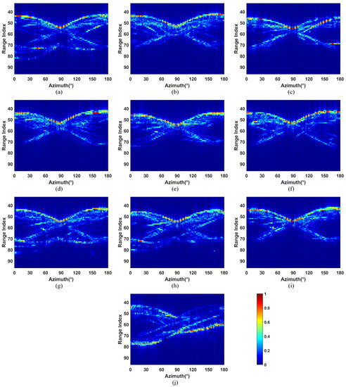
Figure 3. Normalized high-resolution range profiles (HRRPs) of 10 civilian vehicles. (a) Camry; (b) Jeep99; (c) Mitsubishi; (d) MazdaMPV; (e) HondaCivic4dr; (f) Jeep93; (g) Maxima; (h) Sentra; (i) ToyotaAvalon; (j) ToyotaTacoma.

The 8-fold cross-validation was exploited as mentioned before. Consequently, the complete training dataset of each target contained 360 HRRP samples with an azimuth interval of 0.5${}^{\circ }$; and 2520 test samples constituted the test dataset of each target. In each validation, 30 Monte Carlo experiments were conducted.

3.1.2. Recognition Performance of the CPLP Algorithm

In this section, the recognition performance of CPLP algorithm is demonstrated on the simulated data of 10 civilian vehicles. First, the influences of some parameters on the recognition performance are presented. Then, we study the recognition performance versus the size of unlabeled dataset and labeled dataset.

 (1) Parameter Setup

In this section, the effects of the parameters $\alpha$, ${\sigma }^2$, and k in the k-RNN algorithm for computing ${\mathit{W}}_{UL}$ (denoted as $k_1$) and for computing ${\mathit{W}}_{UU}$ (denoted as $k_2$) on the recognition performance of the CPLP algorithm are given. The labeled dataset consists of a tenth of the complete training data, i.e., 36 HRRPs from each target. The unlabeled dataset contains 1000 HRRP samples, i.e., 100 samples randomly selected from the test dataset of each target.

First, we evaluate the influences of parameters $k_1$ and $k_2$ on the recognition performance of the CPLP algorithm. The parameter $k_1$ controls the number of RNNs between labeled and unlabeled samples, and $k_2$ is related to the number of RNNs between unlabeled samples. Let the values of $k_1$ and $k_2$ range from 3 to 20 with interval of 1; the results are shown in Figure 4. We can see that the recognition accuracy first increased and then decreased with increasing $k_1$ and $k_2$, and the best performance was obtained within the range of $k_1\in \left[4,9\right]$ and $k_2\in \left[6,12\right]$. In the following experiments conducted on the data of 10 civilian vehicles, we fixed $k_1=6$ and $k_2=10$.

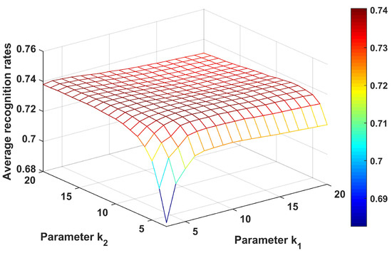
Figure 4. Recognition results of the CPLP algorithm for 10 civilian vehicles with different values of $k_1$ and $k_2$. The parameters $\alpha$ and ${\sigma }^2$ were searched to get the best recognition results.

Next, we analyzed the recognition accuracy under different values of the parameter ${\sigma }^2$ ranging from 0.01 to 0.2 with interval 0.01; the results are shown in Figure 5. Clearly, the recognition rates increased when ${\sigma }^2$ varied from 0.01 to 0.05, and then reduced gradually. Hence, ${\sigma }^2=0.05$ for the following experiments on the data of 10 civilian vehicles.

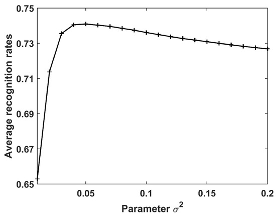
Figure 5. Recognition results of the CPLP algorithm for 10 civilian vehicles in relation to the parameter ${\sigma }^2$. In the experiments, $k_1=6$, and $k_2=10$, and $\alpha$ was used to get the best recognition results.

Finally, the effect of the parameter $\alpha$ was evaluated. The other parameters were fixed as ${\sigma }^2=0.05$, $k_1=6$, and $k_2=10$. As shown in Section 2.2, the parameter $\alpha$ affects the value of ${\mathit{W}}_{UL}^{*}$. We set $\alpha =0,0.3,0.6,0.99$; the computed matrices ${\mathit{W}}_{UL}^{*}$ are shown in Figure 6.

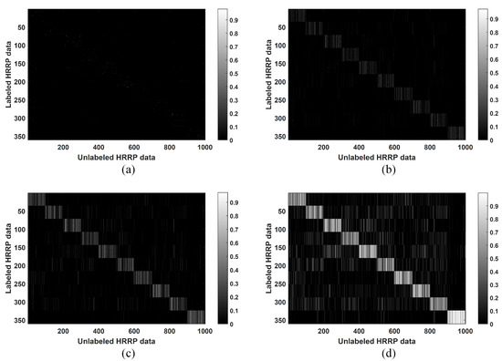
Figure 6. Matrix ${\mathit{W}}_{UL}^{*}$ computed in the CPLP algorithm when $\alpha =0,0.3,0.6,0.99$, respectively. The labeled data and unlabeled data are arranged in the same target order: Camry, 1999 Jeep, Mitsubishi, Mazda MPV, Honda Civic 4dr, 1993 Jeep, Nissan Maxima, Nissan Sentra, Toyota Avalon, and Toyota Tacoma. (a) $\alpha =0$; (b) $\alpha =0.3$; (c) $\alpha =0.6$; (d) $\alpha =0.99$.

As can be seen, with increased $\alpha$, more edges are built between labeled samples and unlabeled ones, and the edge weights become larger. The samples belonging to the same class may not be connected with small $\alpha$, whereas the edges between the samples belonging to different classes may be built when $\alpha$ is large. Both cases above resulted in unsatisfactory recognition performance. Thus, an appropriate value of $\alpha$ is important for the performance of the CPLP algorithm. It should be noted that the matrix ${\mathit{W}}_{UL}^{*}$ degrades to the unsupervised version ${\mathit{W}}_{UL}$ when $\alpha =0$. Hence, the LP algorithm that computes ${\mathit{W}}_{UL}^{*}$ in an unsupervised manner can be regarded as a specialization of the proposed CPLP algorithm.

Figure 7 shows the recognition results when the parameter $\alpha$ varies from 0 to 0.99 with interval 0.01. It can be seen that the recognition accuracy increases gradually when $\alpha \in \left[0,0.4\right]$, then maintains a relatively stable value when $\alpha \in \left(0.4,0.75\right)$, and finally decreases gradually. In the following experiments on the HRRP data of 10 civilian vehicles, $\alpha =0.6$ was chosen.

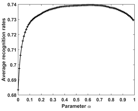
Figure 7. Recognition results of the CPLP algorithm for 10 civilian vehicles with different values of $\alpha$.

 (2) Performance Versus Size of Unlabeled Dataset

The recognition performance of the proposed CPLP algorithm is compared with the LP algorithm in regard to the size of the unlabeled dataset. The number of unlabeled samples of each target ranged from 50 to 500 with interval 50; the recognition results are shown in Figure 8. It can be observed that (1) the recognition accuracy of both methods increased as the size of the unlabeled dataset increased, because more unlabeled samples facilitate more accurate descriptions of data structure; (2) the proposed CPLP algorithm exhibited better performance than the LP algorithm due to the constraint propagation for computing the matrix ${\mathit{W}}_{UL}^{*}$.

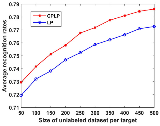
Figure 8. Recognition results of CPLP and label-propagation (LP) algorithms for 10 civilian vehicles in relation to the size of unlabeled dataset of each target. In the experiments, labeled dataset consists of 360 HRRP samples, i.e., 36 HRRP samples from each target. The unlabeled data are randomly selected from test dataset.

 (3) Performance Versus Size of Labeled Dataset

We also conducted experiments to compare the CPLP and LP algorithms under different sizes of labeled dataset. The recognition results for when the number of labeled samples of each target ranged from 24 to 72 with an interval of 12 are shown in Figure 9. We see that the recognition performance became better with the increase in size of the labeled dataset. The reason is that a small labeled dataset is insufficient for discovering the data structure of each target. Moreover, the CPLP algorithm outperformed the LP algorithm, especially for small labeled datasets, because of the constraint propagation for computing the matrix ${\mathit{W}}_{UL}^{*}$.

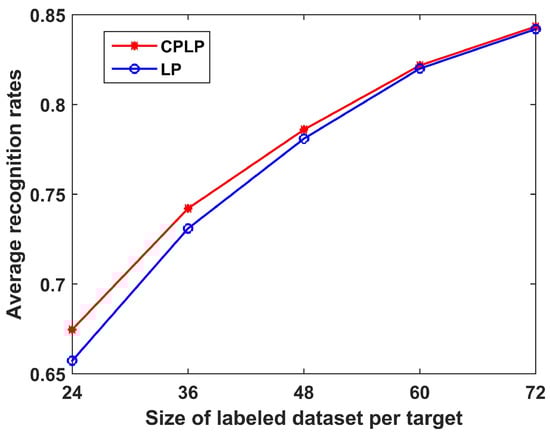
Figure 9. Recognition results of CPLP and LP algorithms for 10 civilian vehicles in relation to the size of the labeled dataset of each target. In the experiments, we randomly selected 100 HRRP samples from the test dataset of each target, yielding 1000 HRPPs in the unlabeled dataset.

3.1.3. Recognition Performance of SLFN with CPLP Method

In this section, the effectiveness of the proposed SLFN with CPLP method is demonstrated on the simulated data of 10 civilian vehicles. First, the recognition performance of the proposed method is investigated with varying sizes of OTD and TDC, and values of parameter p. Then, comparative experiments are shown that were carried out to analyze the proposed method and state-of-the-art methods, including the self-training OS-RKELM method, the OS-RKELM with a SVM, the incremental Laplacian regularization extreme learning machine (ILR-ELM) [33], the SVM, the K-SVD, and the DDAE.

In the following experiments, a Gaussian kernel taking the form of $K\left({\mathit{x}}_1,{\mathit{x}}_2\right)=exp\left(-{∥{\mathit{x}}_1-{\mathit{x}}_2∥}^2/\phantom{{∥{\mathit{x}}_1-{\mathit{x}}_2∥}^{2}a}b\right)$ was selected for Equation (1). The parameter b was set as 0.6, which is the optimal value according to our observations. The TDC was randomly selected from the test dataset. After being learned, it was removed from the test dataset.

 (1) Performance Versus Size of the OTD

In this section, the recognition performance of the proposed SLFN with CPLP method is studied with varying sizes of the OTD. The recognition results with learning steps are shown in Figure 10. As expected, for all the sizes of OTD, the proposed method exhibited increasing recognition performance along learning steps. This indicates that the proposed method can improve the recognition performance by exploiting knowledge from test data. In addition, the larger the size of the OTD, the better the recognition performance, since a large OTD can describe the target signature in more detail.

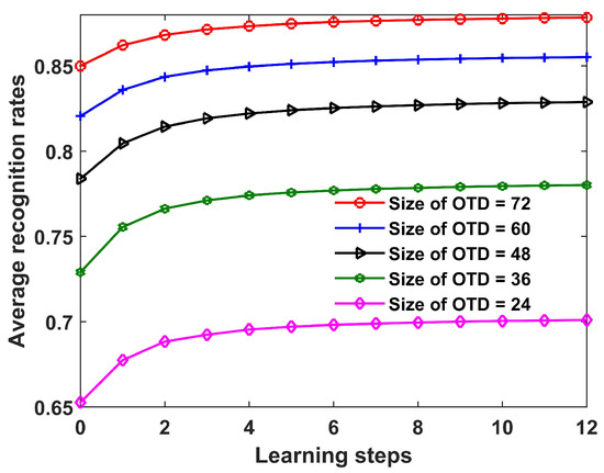
Figure 10. Recognition results of the proposed SLFN with CPLP method for 10 civilian vehicles versus learning steps under different sizes of offline training dataset (OTD). The test data chunk (TDC) contained 200 HRRP samples from each target, and the parameter p was set as 90 in the experiments.

 (2) Performance Versus Size of the TDC

In this section, we study the recognition performance of the proposed method with different sizes of TDC. The results are shown in Figure 11. The observations obtained were as follows. First, for all the sizes of TDC, the recognition performance increased in the update process, which demonstrates the effectiveness of the proposed method. Second, a large size for the TDC yielded a greater improvement of recognition performance. The reason is that the CPLP algorithm exhibits better recognition performance with more test samples, so that the new training data used for updating SLFN parameters contained less error-labeled samples.

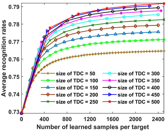
Figure 11. Recognition results for 10 civilian vehicles with number of learned samples per target under different sizes of TDC. In the experiments, the size of OTD from each target was fixed as 36, and the parameter p was set as 100.

 (3) Performance Versus Parameter p

In this section, we study the influence of the parameter p on the recognition performance of the proposed SLFN with CPLP algorithm. Figure 12 shows the recognition results with learning steps under different values of p.

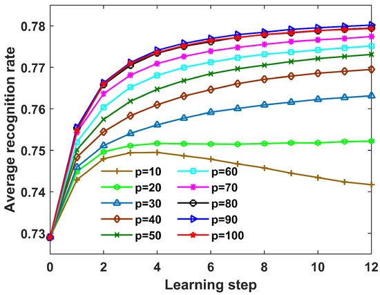
Figure 12. Recognition accuracy of the proposed SLFN with CPLP method for 10 civilian vehicles with learning steps when p ranged from 10 to 100 with an interval of 10. The OTD consisted of a tenth of the complete training data, and the size of TDC from each target was 200.

We observed that (1) when $p\ge 30$, the recognition performance became better and better with learning steps; (2) when $p=10$ and 20, the recognition accuracy first increased and then decreased with learning steps; (3) the recognition performance gained the largest improvement when $p=90$. The reasons are analyzed in what follows. As illustrated in [34], in the update process, the samples with true pseudolabels but low confidence carry more information and contribute more to improving the SLFN performance, whereas employing the samples with high confidence may result in overfitting of classifiers. When p is small, the dataset used for updating the SLFN parameters consists only of the samples with high confidence that match well to the current SLFN and CPLP models, so the SLFN model may overfit the learned samples with learning steps. When p increases, more samples with low confidence are used for updating the SLFN parameters, resulting in larger improvement of recognition performance. However, the number of error-labeled samples also increases with the increasing p, so the recognition performance with $p=100$ is worse than that with $p=90$.

Figure 13 shows the variation of recognition results after the update process with the parameter p. We can see that when the size of the OTD is fixed, the trends in the performance curves of different sizes of TDC are almost the same as with the parameter p. This indicates that the size of the TDC has little effect on the optimal value of p. However, the optimal value of p becomes greater with an increase in the size of the OTD. The reason is that the greater the size of the OTD, the smaller the number of error-labeled samples contained in the TDC. When the size of the OTD of each target is 24, the optimal value of p is 85, so a small number of error-labeled samples were used to update the SLFN parameters. When the size of the OTD of each target goes up to 72, the optimal value of p is 100. The number of error-labeled samples contained in the TDC was small enough that all samples with pseudolabels in TDC were used to update the SLFN parameters.

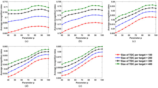
Figure 13. Recognition results for 10 civilian vehicles after the update process under varying values of parameter p. (a) Size of OTD from each target = 24; (b) size of OTD from each target = 36; (c) size of OTD from each target = 48; (d) size of OTD from each target = 60; (e) size of OTD from each target = 72.

 (4) Performance Comparison

The proposed SLFN with CPLP algorithm is evaluated through a comparison with the state-of-the-art methods. Figure 14 shows the recognition results with learning steps under different sizes of OTD and TDC. In addition, we provide the baseline results as an upper bound in which all the test data are labeled correctly and were adopted for updating the SLFN parameters.

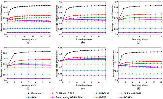
Figure 14. Recognition performances of the proposed SLFN with CPLP method and other methods for 10 civilian vehicles with respect to learning steps; (a) size of OTD per target = 36 and size of TDC per target = 100; (b) size of OTD per target = 36 and size of TDC per target = 200; (c) size of OTD per target = 36 and size of TDC per target = 300; (d) size of OTD per target = 36 and size of TDC per target = 400; (e) size of OTD per target = 72 and size of TDC per target = 200; (f) size of OTD per target = 24 and size of TDC per target = 200.

We found that the proposed method outperforms the other methods at all sizes of TDC and OTD. The recognition accuracy of the self-training OS-RKELM method first increased but then reduced gradually with learning steps. This was because that this method selects the test data with high confidence annotated by itself, which reinforces the bias of current encoded model along learning steps. The SLFN with SVM method exhibited the same trend as the self-training OS-RKELM method on HRRPs of 10 civilian vehicles. The reason for that may be that the SVM classifier only considers the structure of training data but ignores the information involved in the test data. Moreover, it views all the learned test samples as training data for SVM, which accumulates the error-labeled samples and leads to worse recognition performance. The ILR-ELM depends on the manifold assumption to utilize the unlabeled test data. However, this assumption does not hold for all samples, which may actually hurt recognition accuracy. The SVM, K-SVD, and DDAEs algorithms do not utilize test data, so their recognition rates were unchanged during the classification process. Since the SVM method did not utilize all the training samples, it exhibited worse performance than the RKELM algorithm when the training data were not complete. The K-SVD algorithm was not good in terms of recognition performance due to a lack of latent information among training samples for 10 civilian vehicles. For the DDAE algorithm, the limited training data of 10 civilian vehicles were not enough to get the appropriate weights of deep networks, so the overfitting problem could occur and the generalization performance was unsatisfactory.

3.2. Measured Data of 3 Military Vehicles

3.2.1. Dataset Description

In this section, the effectiveness of the proposed method is demonstrated using the measured data of three military vehicles with sizes of $5.8\times 2.9$ m, $5.5\times 2.6$ m and $6.5\times 3$ m, respectively. The measured data were collected in an open field using a radar system placed on a platform 100 m above the ground plane. A stepped-frequency pulsed waveform was transmitted with the stepped frequency interval of 5 MHz and the resultant bandwidth of 640 MHz. Figure 15 shows the top views of geometries of the three military vehicles relative to radar. The first military vehicle was spinning around its center when it was illuminated by electromagnetic waves, and 1991 HRRP samples were collected. The second military vehicle moved following an elliptical path during 1398 HRRP samples being acquired. The echoes of the third vehicle were collected at eight azimuth angles, with 120 HRRP samples collected at each azimuth angle.

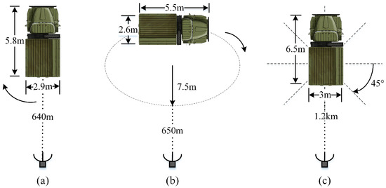
Figure 15. Top views of the geometries of the 3 military vehicles relative to radar. (a) Military vehicle 1; (b) Military vehicle 2; (c) Military vehicle 3.

The 4-fold, 3-fold, and 4-fold cross-validations were exploited for the data of three military vehicles, respectively. As a result, the complete training datasets of the three targets contain 497, 466, and 240 HRRP samples, respectively; and 1494, 932, and 720 samples respectively constitute the test dataset of the three vehicles. In the following experiments, 80 Monte Carlo experiments were conducted in each validation.

3.2.2. Recognition Performance of CPLP Algorithm

The recognition performance of the CPLP algorithm was studied on the data of three military vehicles. First, the effects of some parameters is given. Then, the performance versus the size of unlabeled dataset and labeled dataset is analyzed.

 (1) Parameter Setup

In this section, we present the impact of the parameters $\alpha$, ${\sigma }^2$, $k_1$ and $k_2$, on the recognition performance using the measured data of three military vehicles. The labeled dataset consists of a tenth of the complete training data, i.e., 47 HRRPs from the first target, 50 HRRPs from the second target, and 24 HRRPs from the third target. The unlabeled dataset contains 300 HRRP samples, i.e., 100 samples randomly selected from the test data of each target.

First, we analyze the effect of the parameters $k_1$ and $k_2$. In the experiments, the parameter $k_1$ varied from 10 to 100 with interval of 1, and the parameter $k_2$ ranged from 1 to 30 with an interval of 1. The average recognition rates are shown in Figure 16. As shown, the CPLP algorithm achieved higher performance at $k_1\in \left[42,48\right]$ and $k_2=4$. In the following experiments conducted on the measured data of three military vehicles, $k_1=46$ and $k_2=4$ were chosen.

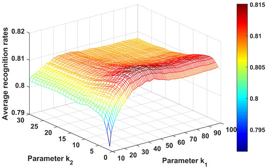
Figure 16. Recognition results of CPLP algorithm for 3 military vehicles with different values of $k_1$ and $k_2$. In the experiments, The parameters ${\sigma }^2$ and $\alpha$ were searched to provide the best recognition performance.

The performance of the CPLP algorithm with the parameter ${\sigma }^2$ is evaluated next. Figure 17 shows the recognition results. Clearly, the recognition accuracy first increased and then decreased. The best performance was achieved at 0.06. In the following experiments conducted on the measured data of three military vehicles, ${\sigma }^2=0.06$ was chosen.

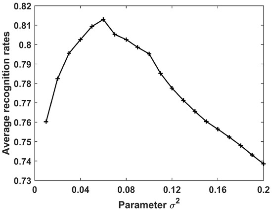
Figure 17. Recognition results of CPLP algorithm for 3 military vehicles with parameter ${\sigma }^2$. The parameter $\alpha$ is searched to acquire the best results in the experiments.

Finally, the impact of the parameter $\alpha$ is analyzed. The constructed matrices ${\mathit{W}}_{UL}^{*}$ are shown in Figure 18 when $\alpha =0,0.35,0.7$ and 0.99. We can see that a large $\alpha$ leads to more edges constructed and larger edge weights, which is the same as what was observed in Figure 6.

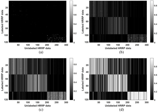
Figure 18. Matrix ${\mathit{W}}_{UL}^{*}$ computed in the CPLP algorithm using the measured data of 3 military vehicles when $\alpha =0,0.35,0.7,$ and $0.99$. The labeled data and unlabeled data are arranged in the same target order. (a) $\alpha =0$; (b) $\alpha =0.35$; (c) $\alpha =0.7$; (d) $\alpha =0.99$.

Figure 19 shows the recognition accuracy when $\alpha$ ranges from 0 to 0.99 with interval of 0.01. We can see that both large and small values of $\alpha$ result in degradation of recognition performance. The best recognition performance was achieved when $\alpha \in \left[0.26,0.4\right]$. In the following experiments conducted on the measured data of three military vehicles, $\alpha =0.32$ was chosen.

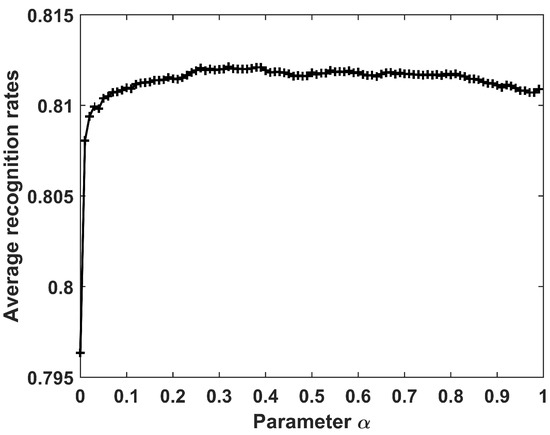
Figure 19. Recognition results of CPLP algorithm for 3 military vehicles versus parameter $\alpha$.

 (2) Performance Versus Size of Unlabeled Dataset

The performance of the CPLP and LP algorithms is studied versus the size of unlabeled dataset. The recognition results are presented in Figure 20 for when the number of unlabeled samples of each target varied from 50 to 250 with interval of 50. It is shown that the recognition accuracy of both methods became better with a larger size of unlabeled dataset. Moreover, because of the constraint propagation for the matrix ${\mathit{W}}_{UL}^{*}$, the proposed CPLP algorithm showed greater recognition accuracy than the LP algorithm.

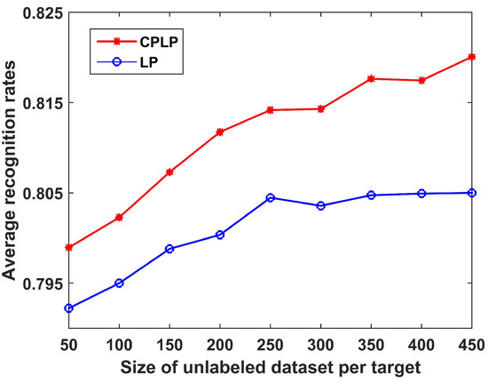
Figure 20. Recognition results of CPLP and LP algorithm for three military vehicles versus size of unlabeled dataset. In the experiments, a tenth of the complete training data constituted the labeled dataset.

 (3) Performance Versus Size of Labeled Dataset

We compare the recognition performance of the CPLP with LP algorithms versus the size of labeled dataset. The recognition results are shown in Figure 21 for when the size of the labeled dataset ranged from 60 to 300 with an interval of 60. It is shown that the recognition rates become higher when the size of the labeled dataset increases, and the proposed CPLP algorithm outperformed the LP algorithm at all sizes of the labeled dataset.

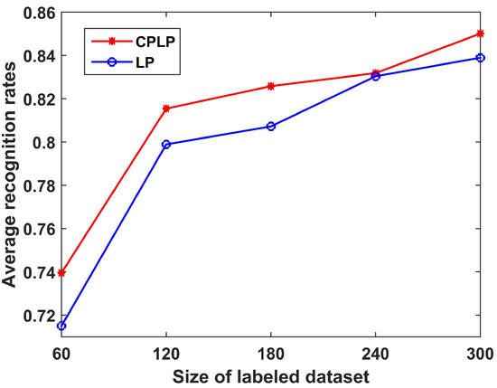
Figure 21. Recognition results of CPLP and LP algorithms for three military vehicles versus size of labeled dataset. In the experiments, the unlabeled dataset of each target contained 100 HRRP samples randomly selected from the test dataset.

3.2.3. Recognition Performance of SLFN with CPLP Method

In this section, the superiority of the SLFN with CPLP method is demonstrated on the measure data from three military vehicles. First, the effects of the size of OTD, size of TDC, and parameter p on the recognition performance are analyzed. Comparative experiments were conducted too.

In Equation (1), the optimal parameter b is 0.5 according to our observation. The TDC contained samples selected randomly from the test dataset. After being learned, they were removed from the test dataset.

 (1) Performance Versus Size of OTD

In this section, the recognition performance of the proposed method for three military vehicles is studied under different sizes of OTD. Figure 22 plots the recognition results with learning steps. As can be seen, the performance of the proposed method improves with learning steps, which indicates its effectiveness. Furthermore, more offline training samples lead to higher recognition rates, which is in agreement with the previous analysis.

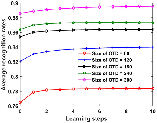
Figure 22. Recognition results of the proposed SLFN with CPLP method for three military vehicles versus learning steps under different sizes of OTD. In the experiments, The TDC contained a total of 300 samples.

 (2) Performance Versus Size of TDC

The recognition performance of the proposed method for three military vehicles under different sizes of TDC is studied in this section. The recognition results are shown in Figure 23. As is seen, the recognition rates increase with learning steps for all the sizes of TDC, which verifies the effectiveness of the proposed method. Moreover, the TDC containing more samples yielded better performance, which is consistent with observations from Figure 11.

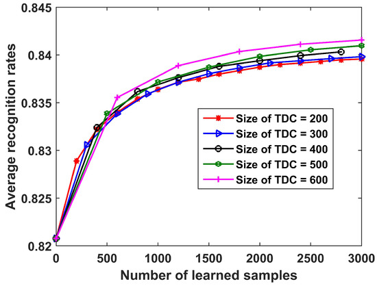
Figure 23. Recognition results of the proposed SLFN with CPLP method for 3 military vehicles versus learning steps under different sizes of TDC. In the experiments, the size of OTD was fixed as 120.

 (3) Performance with Parameter p

In this section, the influence of the parameter p on recognition performance of the SLFN with CPLP algorithm is studied on the measured data of three military vehicles. The recognition results with learning steps under different values of p are presented in Figure 24. We observe that (1) when the size of OTD = 120, the recognition rates increase with learning steps under all the value of p, and the greatest improvement of recognition performance is gained at p = 80; (2) when the size of OTD = 240, the recognition rates increase with learning steps when $p\ge 30$, and the recognition performance achieves the best at p = 90. These phenomena demonstrate the effectiveness of the proposed method, and the reason is illustrated in Section 3.1.3.

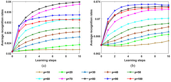
Figure 24. Recognition accuracy of the proposed SLFN with CPLP method for 3 military vehicles with learning steps when p ranges from 10 to 100 with an interval of 10. In the experiments, the size of TDC = 300. (a) Size of OTD = 120; (b) size of OTD = 240.

Figure 25 shows the recognition results for three military vehicles after update process versus the parameter p. As expected, the optimal value of the parameter p is little influenced by the size of TDC, but is affected by the size of OTD. The more offline training samples, the greater the parameter p.

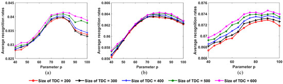
Figure 25. Recognition results for 3 military vehicles after update process under varying values of parameter p. (a) Size of OTD = 120; (b) size of OTD = 180; (c) size of OTD = 240.

 (4) Performance Comparison

The following experiments examined the performances of the proposed method and other methods on the measured data. Figure 26 presents the recognition results with learning steps under different sizes of OTD and TDC. Obviously, the proposed method exceeds the compared methods at all the sizes of OTD and TDC. When the size of OTD = 120, the DDAEs algorithm exhibits better performance than the proposed method before the update, but is not competing with the proposed method along the learning process.

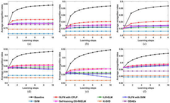
Figure 26. Recognition performances of the proposed SLFN with CPLP algorithm and other methods for 3 military vehicles versus learning steps. (a) Size of OTD = 60 and size of TDC = 300; (b) size of OTD = 120 and size of TDC = 300; (c) size of OTD = 120 and size of TDC = 500; (d) size of OTD = 180 and size of TDC = 300; (e) size of OTD = 240 and size of TDC = 300; (f) size of OTD = 300 and size of TDC = 300.

3.3. Computation Analysis

In the online stage, the proposed SLFN with CPLP method comprises two stages, i.e., the pseudolabel assignment for test data and SLFN parameter update by OS-RKELM algorithm. For the sake of clarity, we analyze the computational complexity of these two stages.

The pseudolabel assignment for test data comprises the prediction by the SLFN, the prediction by the CPLP algorithm, and decision fusion of SLFN and CPLP algorithms. Let L be the length of HRRP, then the computational complexity of the SLFN is $O\left(N_u{N}_l\left(L+C\right)\right)$. For the CPLP algorithm, the most time consuming parts are the KRNN graph construction for computing ${\mathit{W}}_{UU}$ and ${\mathit{W}}_{UL}$, construction for ${\mathit{W}}_{UL}^{*}$, and computation for ${\mathit{F}}_m^U$ by Equation (7). The KRNN graph construction has the computational complexity in the order of $O\left(N_u^{2}lo{g}_2{N}_u\right)$. The construction for ${\mathit{W}}_{UL}^{*}$ has the running time of $O\left(N_u^3+N_u{N}_l^2+N_u^2{N}_l\right)$. The time for computing ${\mathit{F}}_m^U$ has the complexity of $O\left(N_u^3+N_u^2{N}_l+N_u{N}_{l}C\right)$. Thus the CPLP algorithm has the computational complexity in the order of $O\left(N_u^3+N_u^2{N}_l+N_u{N}_l^2+N_u{N}_{l}C+N_u^{2}lo{g}_2{N}_u\right)$. For the decision fusion of SLFN and CPLP algorithms, the computational complexity is $O\left({\left(N_u+N_l\right)}^{2}lo{g}_2\left(N_u+N_l\right)\right)$.

For the SLFN parameter update by the OS-RKELM algorithm, the computational complexity is $O\left(N_l\left(N_l^2+N_u^2+N_l{N}_u\right)\right)$ [24].

Table 1 and Table 2 show the average computational time of the proposed method and the compared methods on the simulated HRRP data of 10 civilian vehicles and measured HRRP data of three military vehicles, respectively. Clearly, the computational time increases with the increase in the size of TDC and OTD. Due to the SVM training process, the SLFN with SVM method is the most time-consuming of all the recognition methods. The proposed SLFN with CPLP method takes less time than the SLFN with SVM method, but takes more time than the ILR-ELM and self-training OS-RKELM methods due to the CPLP algorithm. The SVM, K-SVD and DDAEs algorithms only classify samples and do not update the parameters of classifiers in the test phase, so they take much less time than the update methods.

Table 1. Average computational times of the proposed SLFN with CPLP method and other methods on the HRRP dataset of 10 civilian vehicles.

Size of OTD	Size of TDC	SLFN with CPLP (s)	ILR-ELM (s)	SLFN with SVM (s)	OS-RKELM Self-Training (s)	SVM (ms)	K-SVD (ms)	DDAEs (ms)
240	1000	0.521	0.221	13.637	0.211	0.906	0.968	5.338
	2000	1.398	0.381	13.953	0.351
	3000	3.000	0.623	14.543	0.543
	4000	5.335	0.931	15.070	0.811
360	1000	0.609	0.276	15.160	0.305	0.968	0.975	7.024
	2000	1.570	0.455	15.281	0.520
	3000	3.218	0.707	15.702	0.867
	4000	5.696	1.036	16.724	1.420
720	1000	0.897	0.477	19.220	0.595	1.106	0.983	7.297
	2000	1.953	0.687	19.515	1.244
	3000	3.828	0.960	21.021	2.473
	4000	6.451	1.373	22.911	4.251

Table 2. Average computational times of the proposed SLFN with CPLP method and other methods on the HRRP dataset of 3 military vehicles.

Size of OTD	Size of TDC	SLFN with CPLP (s)	ILR-ELM (s)	SLFN with SVM (s)	OS-RKELM Self-Training (s)	SVM (ms)	K-SVD (ms)	DDAEs (ms)
60	200	0.078	0.014	0.344	0.008	0.228	0.300	5.317
	300	0.100	0.022	0.356	0.012
	500	0.154	0.041	0.365	0.020
120	200	0.080	0.015	0.396	0.011	0.294	0.304	6.309
	300	0.103	0.023	0.397	0.017
	500	0.156	0.041	0.405	0.032
240	200	0.082	0.017	0.463	0.018	0.308	0.306	7.077
	300	0.103	0.025	0.465	0.026
	500	0.163	0.047	0.471	0.041

4. Conclusions

A novel dynamic learning strategy based on the SLFN with assistance from the CPLP algorithm was proposed to tackle the HRRP target recognition task with limited training data. In the offline training phase, the initial parameters of SLFN are obtained with the training data. In the classification phase, the collected test data are first labeled by fusing the recognition results of current SLFN and CPLP algorithms. Then the test samples with reliable pseudolabels are used as additional training data to update the SLFN parameters by the OS-RKELM algorithm. The proposed method dynamically accumulates knowledge from training and test data through online learning, thereby reinforcing the performance of the RATR system with limited training data. In the experiments, the superiority of the SLFN with CPLP method was demonstrated on the simulated HRRP data from 10 civilian vehicles and real HRRP data from three military vehicles.

In the future, more PR methods should be investigated to improve the accuracy of pseudolabels of test data, and other online learning methods should be studied to deal with the RATR problem with limited training data. Moreover, we want to extend our work to the polarimetric HRRP-based RATR.

References

- Ran, L.; Liu, Z.; Xie, R.; Zhang, L. Focusing high-squint synthetic aperture radar data based on factorized back-projection and precise spectrum fusion. Remote Sens. 2019, 11, 2885. [Google Scholar] [CrossRef]
- Zhang, X.; Shi, Y.; Bao, Z. A new feature vector using selected bispectra for signal classification with application in radar target recognition. IEEE Trans. Signal Process. 2001, 49, 1875–1885. [Google Scholar] [CrossRef]
- Du, L.; Liu, H.; Bao, Z.; Xing, M. Radar HRRP target recognition based on higher order spectra. IEEE Trans. Signal Process. 2005, 53, 2359–2368. [Google Scholar]
- Wang, J.; Liu, Z.; Li, T.; Ran, L.; Xie, R. Radar HRRP target recognition via statistics-based scattering center set registration. IET Radar Sonar Navig. 2019, 13, 1264–1271. [Google Scholar] [CrossRef]
- Du, L.; He, H.; Zhao, L.; Wang, P. Noise robust radar HRRP target recognition based on scatterer matching algorithm. IEEE Sensors J. 2016, 16, 1743–1753. [Google Scholar] [CrossRef]
- Jacobs, S.P.; O’Sullivan, J.A. Automatic target recognition using sequences of high resolution radar range-profiles. IEEE Trans. Aerosp. Electron. Syst. 2000, 36, 364–381. [Google Scholar] [CrossRef]
- Copsey, K.; Webb, A. Bayesian gamma mixture model approach to radar target recognition. IEEE Trans. Aerosp. Electron. Syst. 2003, 39, 1201–1217. [Google Scholar] [CrossRef]
- Du, L.; Liu, H.; Bao, Z.; Zhang, J. A two-distribution compounded statistical model for radar HRRP target recognition. IEEE Trans. Signal Process. 2006, 54, 2226–2238. [Google Scholar]
- Feng, B.; Chen, B.; Liu, H. Radar HRRP target recognition with deep networks. Pattern Recogn. 2017, 61, 379–393. [Google Scholar] [CrossRef]
- Pan, M.; Jiang, J.; Kong, Q.; Shi, J.; Sheng, Q.; Zhou, T. Radar HRRP target recognition based on t-SNE segmentation and discriminant deep belief network. IEEE Geosci. Remote Sens. Lett. 2017, 14, 1609–1613. [Google Scholar] [CrossRef]
- Liao, X.; Runkle, P.; Carin, L. Identification of ground targets from sequential high-range-resolution radar signatures. IEEE Trans. Aerosp. Electron. Syst. 2002, 38, 1230–1242. [Google Scholar] [CrossRef]
- Burges, C.J.C. A tutorial on support vector machines for pattern recognition. Data Min. Knowl. Discovery 1998, 2, 121–167. [Google Scholar] [CrossRef]
- Li, L.; Liu, Z.; Tao, L. Radar high resolution range profile recognition via multi-SV method. J. Syst. Eng. Electron. 2017, 28, 879–889. [Google Scholar] [CrossRef]
- Feng, B.; Du, L.; Liu, H.; Li, F. Radar HRRP target recognition based on K-SVD algorithm. In Proceedings of the 2011 IEEE CIE International Conference on Radar, Chengdu, China, 24–27 October 2011; pp. 642–645. [Google Scholar]
- Feng, B.; Du, L.; Shao, C.; Wang, P.; Liu, H. Radar HRRP target recognition based on robust dictionary learning with small training data size. In Proceedings of the 2013 IEEE Radar Conference (RadarCon13), Ottawa, ON, Canada, 29 April–3 May 2013; pp. 1–4. [Google Scholar]
- Du, L.; Liu, H.; Wang, P.; Feng, B.; Pan, M.; Bao, Z. Noise robust radar HRRP target recognition based on multitask factor analysis with small training data size. IEEE Trans. Signal Process. 2012, 60, 3546–3559. [Google Scholar]
- Pan, M.; Jiang, J.; Li, Z.; Cao, J.; Zhou, T. Radar HRRP recognition based on discriminant deep autoencoders with small training data size. Electron. Lett. 2016, 52, 1725–1727. [Google Scholar]
- Yver, B. Online semi-supervised learning: Application to dynamic learning from RADAR data. In Proceedings of the 2009 International Radar Conference “Surveillance for a Safer World” (RADAR 2009), Bordeaux, France, 12–16 October 2009; pp. 1–6. [Google Scholar]
- Zhu, X.; Ghahramani, Z. Learning from labeled and unlabeled data with label propagation. Tech. Rep. 2002, 3175, 237–244. [Google Scholar]
- Bordes, A.; Ertekin, S.; Weston, J.; Bottou, L. Fast kernel classifiers with online and active learning. J. Mach. Learn. Res. 2005, 6, 1579–1619. [Google Scholar]
- Zhang, R.; Rudnicky, A.I. A new data selection principle for semi-supervised incremental learning. In Proceedings of the 18th International Conference on Pattern Recognition (ICPR’06), Hong Kong, China, 20–24 August 2006; pp. 780–783. [Google Scholar]
- Cui, Z.; Tang, C.; Cao, Z.; Dang, S. SAR unlabeled target recognition based on updating CNN with assistant decision. IEEE Geosci. Remote Sens. Lett. 2018, 15, 1585–1589. [Google Scholar] [CrossRef]
- Deng, W.; Ong, Y.-S.; Zhang, Q. A fast reduced kernel extreme learning machine. Neural Netw. 2016, 76, 29–38. [Google Scholar] [CrossRef]
- Deng, W.; Ong, Y.-S.; Tan, P.S.; Zheng, Q. Online sequential reduced kernel extreme learning machine. Neurocomputing 2016, 174, 72–84. [Google Scholar] [CrossRef]
- Belkin, M.; Niyogi, P. Laplacian eigenmaps for dimensionality reduction and data representation. Neural Comput. 2003, 15, 1373–1396. [Google Scholar] [CrossRef]
- Liu, W.; Zhang, T. Bidirectional label propagation over graphs. Int. J. Softw. Inform. 2013, 7, 419–433. [Google Scholar]
- Gong, C.; Fu, K.; Wu, Q.; Tu, E.; Yang, J. Semi-supervised classification with pairwise constraints. Neurocomputing 2014, 139, 130–137. [Google Scholar] [CrossRef]
- Qin, D.; Gammeter, S.; Bossard, L.; Quack, T.; Gool, L.V. Hello neighbor: Accurate object retrieval with k-reciprocal nearest neighbors. In Proceedings of the 2011 Conference on Computer Vision and Pattern Recognition (CVPR), Providence, RI, USA, 20–25 June 2011; pp. 777–784. [Google Scholar]
- Zhong, Z.; Zheng, L.; Cao, D.; Li, S. Re-ranking person re-identification with k-reciprocal Encoding. In Proceedings of the 2017 IEEE Conference on Computer Vision and Pattern Recognition (CVPR), Honolulu, HI, USA, 21–26 July 2017; pp. 3652–3661. [Google Scholar]
- Liu, W.; Tian, X.; Tao, D.; Liu, J. Constrained metric learning via distance gap maximization. Proc. Nat. Conf. Artif. Intell. (AAAI) 2010, 24, 1. [Google Scholar]
- Chen, B.; Liu, H.; Bao, Z. Analysis of three kinds of classification based on different absolute alignment methods. Mod. Radar 2006, 28, 58–62. [Google Scholar]
- Dungan, K.E.; Austin, C.; Nehrbass, J.; Potter, L.C. Civilian vehicle radar data demos. SPIE Proc. 2010, 7699, 731–739. [Google Scholar] [CrossRef]
- Yang, L.; Yang, S.; Li, S.; Liu, Z.; Jiao, L. Incremental laplacian regularization extreme learning machine for online learning. Appl. Soft Comput. 2017, 59, 546–555. [Google Scholar] [CrossRef]
- Zhang, Y.; Er, M.J. Sequential active learning using meta-cognitive extreme learning machine. Neurocomputing 2016, 173, 835–844. [Google Scholar] [CrossRef]
Publisher’s Note: MDPI stays neutral with regard to jurisdictional claims in published maps and institutional affiliations. |
© 2021 by the authors. Licensee MDPI, Basel, Switzerland. This article is an open access article distributed under the terms and conditions of the Creative Commons Attribution (CC BY) license (http://creativecommons.org/licenses/by/4.0/).