Abstract
In this paper, we build on past efforts with regard to the implementation of an efficient feature tracking algorithm for the mass processing of satellite images. This generic open-source feature tracking routine can be applied to any type of imagery to measure sub-pixel displacements between images. The routine consists of a feature tracking module (autoRIFT) that enhances computational efficiency and a geocoding module (Geogrid) that mitigates problems found in existing geocoding algorithms. When applied to satellite imagery, autoRIFT can run on a grid in the native image coordinates (such as radar or map) and, when used in conjunction with the Geogrid module, on a user-defined grid in geographic Cartesian coordinates such as Universal Transverse Mercator or Polar Stereographic. To validate the efficiency and accuracy of this approach, we demonstrate its use for tracking ice motion by using ESA’s Sentinel-1A/B radar data (seven pairs) and NASA’s Landsat-8 optical data (seven pairs) collected over Greenland’s Jakobshavn Isbræ glacier in 2017. Feature-tracked velocity errors are characterized over stable surfaces, where the best Sentinel-1A/B pair with a 6 day separation has errors in X/Y of 12 m/year or 39 m/year, compared to 22 m/year or 31 m/year for Landsat-8 with a 16-day separation. Different error sources for radar and optical image pairs are investigated, where the seasonal variation and the error dependence on the temporal baseline are analyzed. Estimated velocities were compared with reference velocities derived from DLR’s TanDEM-X SAR/InSAR data over the fast-moving glacier outlet, where Sentinel-1 results agree within 4% compared to 3–7% for Landsat-8. A comprehensive apples-to-apples comparison is made with regard to runtime and accuracy between multiple implementations of the proposed routine and the widely-used “dense ampcor" program from NASA/JPL’s ISCE software. autoRIFT is shown to provide two orders of magnitude of runtime improvement with a 20% improvement in accuracy.
1. Introduction
Knowledge of glacier and ice sheet displacement is important to refine our knowledge of glacier mechanics and responses to environmental forcing. Among various methods, spaceborne radar and optical imagery have been widely used to determine ice displacement at high spatial and temporal resolution with large-scale spatial coverage [1,2]. Over fast-moving ice surfaces, displacement is typically measured using feature (or speckle) tracking between a pair of images [3,4,5,6,7,8,9,10,11]. For radar imagery, Synthetic Aperture Radar Interferometry (InSAR) techniques can also be used to determine the line-of-sight surface displacement between a pair of images [12,13,14,15,16,17,18,19,20]. Results from both approaches can be combined to provide an optimal estimate of ice motion [21,22,23,24].
Studies have investigated the results obtained using various feature tracking programs, as well as results obtained using InSAR techniques [25]. One of the most widely used feature tracking algorithms is the amplitude cross-correlator (“ampcor") developed by NASA/JPL. ampcor is an open-source software that has been integrated to NASA/JPL’s open-source InSAR processing software, such as ROI_PAC [26] and the InSAR Scientific Computing Environment (ISCE) [27], which were further used to develop various feature tracking software found in the literature [25,28,29,30,31,32,33].
This paper focuses on the efficient implementation of the feature tracking method and presents a generic open-source feature tracking routine (Available at: https://github.com/leiyangleon/autoRIFT (accessed on 10 January 2021)). We note here that the motivation of this work is not to improve the accuracy of the feature tracking method or to improve on current normalized cross-correlation algorithms; instead, our motivation is to build on past efforts with the implementation of an efficient feature tracking algorithm for the mass processing of satellite images. As described in Section 2, the routine consists of two modules: (1) the feature tracking module, autoRIFT, which was first presented in [34] to improve computational efficiency, is summarized here with several refinements; and (2) a geocoding module, Geogrid, is introduced so that autoRIFT is able to run on any geographic Cartesian coordinate grid without causing problems such as a loss of information and/or image distortion as found in existing geocoding algorithms. In Section 3, to validate the efficiency and accuracy of this routine, we demonstrate its use by utilizing ESA’s Sentinel-1A/B radar data and NASA’s Landsat-8 optical data for tracking ice motion and examine the performance (runtime and accuracy) of the proposed routine by benchmark against the state-of-the-art ampcor program. This paper concludes with Section 4 and Section 5, which provide further discussions and conclusions regarding the design and techniques employed by the feature tracking routine. Auxiliary derivations for the geocoding module can be found in Appendix A and Appendix B.
2. Methodology
2.1. autoRIFT: The Feature Tracking Module
The feature tracking algorithm called autoRIFT (autonomous Repeat Image Feature Tracking) was first presented in [34] to improve the computational efficiency of the feature tracking of repeat images. This algorithm finds the displacement between two images with a nested grid design, sparse/dense combinative searching strategy and disparity filtering technique, which are summarized below with several refinements.
From the two images, the source (also called the reference) and template (also called the chip) image patches are extracted over a sampling grid and matched by identifying the peak normalized cross-correlation (NCC) value. autoRIFT employs iteratively progressive chip sizes, as illustrated in Figure 1a. When a particular chip size fails to estimate the displacements, the signal to noise ratio can be increased by enlarging the size of the search chip. In all cases, the minimum successful chip size is selected, ensuring the maximum effective resolution of the displacement output. For the chip size to progress iteratively, a nested grid design (as illustrated in Figure 1b) is developed where the original (highest resolution) chip size can be iteratively enlarged by a factor of two. Pixel displacements estimated with a larger chip size are performed on a coarser grid that is resampled and posted on the grid of the finest chip size.
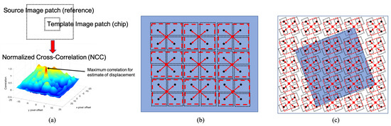
Figure 1.
(a) Template matching using normalized cross-correlation, and (b,c) the nested grid design in autonomous Repeat Image Feature Tracking (autoRIFT), where (b) shows the image grid and (c) shows the geographic grid. In (b,c), original chips are shown as black, dotted rectangles with the center grid point as a black dot, and chips enlarged by a factor of two (that iteratively progresses) are shown as red, dashed rectangles with the center grid point as a red dot.
During the execution of each unique chip size, a sparse search is first performed with an integer pixel accuracy at a downsampled grid. This is done to exclude areas of “low-coherence" or a low signal to noise ratio, where the pixel displacement tracking is unreliable. Following the sparse search, a dense search is sequentially performed with sub-pixel accuracy and is guided by the results of the sparse search. Finding the sub-pixel displacement involves oversampling the NCC correlation surface to identify a refined location for the peak correlation. Most oversampling approaches are prone to pixel-locking, which can bias the sub-pixel displacement estimate [35]. autoRIFT estimates sub-pixel displacement using a fast Gaussian pyramid upsampling algorithm that is robust to sub-pixel locking, where an adjustable oversampling ratio of 64 is used by default to resolve to a precision of 1/64 pixel.
autoRIFT uses the Normalized Displacement Coherence (NDC) filter [34] to identify and remove low-coherence displacement results based on displacement disparity thresholds that are scaled to the local search distance. In other words, displacement results are masked out if their local median absolute deviation (MAD) is beyond the normalized displacement disparity threshold. Scaling the threshold to the local search distance has the benefit of normalizing changes in the magnitude of the noise that scale with changes in the search distance.
autoRIFT also allows users to specify the search center (center of the reference), search distance (size of the reference), the downstream search displacement (center displacement of the chip with respect to the reference) and iteratively progressive chip sizes (with minimum and maximum specified, iteratively progressing by a factor of two), as well as the number of disparity filter parameters that are beneficial for the efficient use of autoRIFT. In particular, the downstream search displacement, search distance, minimum chip size and maximum chip size can be spatially varied to accommodate regions with differing mean velocities and variability. For example, 1) using the initial estimate of downstream search displacement remarkably reduces the search distance over fast-moving targets, and 2) a small search distance with large chip size (coarse resolution) is well suited for resolving low-gradient, slow-moving surfaces, while a large search distance with a small chip size (high resolution) is required to resolve fast-moving targets with steep spatial gradients.
These model features result in the maximum extraction of inter-image displacements with improved accuracy. They also provide greatly reduced computational overhead, allowing for the mass autonomous processing of large image archives without manual tuning of search parameters.
Several refinement techniques have been incorporated recently. The oversampling ratio for the sub-pixel program can also be adaptively selected as a function of the chip size. For example, for very slow motion, a large chip size can be used to increase the signal to noise ratio of the NCC, justifying the use of a higher precision sub-pixel displacement estimator that can be obtained using a larger oversample ratio (e.g., 128). Multiple image pre-filtering options are also provided, allowing for the feature tracking of texture and long-wavelength features (e.g., useful when topographic shading is a desired feature), as well as the feature tracking with only texture (e.g., high-pass filtering, which minimizes the correlation to topographic shading but is prone to temporal decorrelation). Other pre-processing options include converting the amplitude images to different data types (e.g., an 8-bit unsigned integer or 32-bit single precision float). In particular, the combination of high-pass filtering and conversion to an 8-bit unsigned integer further improves the computational efficiency without compromising accuracy. The core processing in autoRIFT (i.e., NCC and image pre-processing) calls OpenCV’s Python and C++ functions and has been parallelized with the capability of multithreading for further efficiency.
2.2. Geogrid: The Geocoding Module
When applying feature tracking to remote sensing imagery, it is always desired for the computed displacements to be geocoded from the image coordinates to geographic coordinates. Typically, there are two ways to geocode feature tracking outputs: the first one geocodes the repeat images first and directly runs feature tracking in the geographic coordinates, while the second one runs feature tracking on an image coordinate grid, which is then geocoded to geographic coordinates. However, in both ways, either a repeat image or displacement field is interpolated/resampled from image coordinates to geographic coordinates. Such transformations are costly and result in a loss of information and/or image distortion, e.g., over the shear margin of glacier outlets.
To overcome these limitations, we develop a new geocoding algorithm for feature tracking outputs, which runs feature tracking in the native image coordinates but directly over a geographic coordinate grid (not interpolated/resampled from an image coordinate grid, as performed by the second method above).
In particular, a geocoding module, Geogrid, has been developed for one-to-one mapping (via two look-up tables) between pixel index and displacement in the image coordinates and geolocation and velocity in the geographic coordinates , with X and Y being easting and northing, respectively. Here, velocity represents the displacement (in the unit of meter) divided by the time separation of the image pair. Therefore, the feature tracking is performed in the native image coordinates, then mapped to geographic coordinates, both of which are done directly over a geographic coordinate grid.
To utilize the Geogrid module, users first need to define a grid in geographic Cartesian coordinates; e.g., Universal Transverse Mercator or Polar Stereographic. Then, the image coordinate information needs to be known; e.g., radar orbit information for radar imagery and map projection information for Cartesian-coordinate imagery. By using the image coordinate information, along with the Digital Elevation Model (DEM) for the projection of radar data, a look-up table between the pixel index in image coordinates and the geolocation in the geographic coordinates can be obtained for each point on the geographic grid.
As illustrated in Figure 2, suppose a small increment is given to each dimension of the image coordinates, (or ); this in turn results in a small displacement in geographic coordinates through coordinate transformation. Here, we denote the resulting unit vector of displacement in geographic coordinates as (or ). By using the unit vectors, and , any map velocity vector (denoted as ) can be related to pixel displacement and as below:
where is the time separation of the image pair. Note that is a vector notation and denotes a unit vector. Further, when local surface slopes ( and ) are also provided, the unit vector of the surface normal can be expressed as [36]. By using the slope parallel assumption, where surface displacement is assumed to be parallel to the local surface; i.e.,
the Z-direction (vertical) velocity can be expressed as a function of the X and Y-direction displacement velocities. After rearranging the terms, (1)–(3) can be concisely written as
where the conversion matrix is derived in Appendix A.
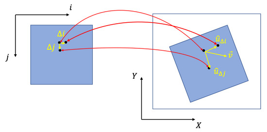
Figure 2.
Look-up tables in Geogrid for one-to-one mapping between image coordinates and geographic coordinates . Given a small increment in the i-direction (or in j-direction) and through coordinate transformation, the unit vector of the induced displacement in is (or ).
As illustrated in Figure 2, this provides a translation (another look-up table) between pixel displacement ( and ) in image coordinates and velocity ( and ) in geographic coordinates. By inverting (4), this module can also be used to estimate the downstream search displacement ( and ) in image coordinates given an expected (reference) velocity ( and ) in geographic coordinates.
A DEM is required in the above mapping between radar viewing geometry and the geographic coordinate system, but results are relatively insensitive to DEM errors (a DEM change or error of a few tens of meters results in pixel mis-registration on the order of 0.001 pixels). Therefore, error resulting from the elevation change between image acquisitions or the DEM itself do not have a large impact on the co-registration (thus, the estimated displacements) of the radar images. In contrast, an orbit precision of centimeter accuracy is required to ensure good co-registration. Note that a DEM is not required for the application of Geogrid to optical imagery.
It should be noted that when the slope parallel assumption fails, there is an error propagation from the vertical velocity to the converted horizontal velocities; i.e.,
where is the vertical velocity error by using slope parallel assumption, and are the propagated error of horizontal velocities in X and Y directions and P and Q are the propagation coefficients as derived in Appendix B. From (5) and Appendix B, it is shown that the error propagation is linear and the linear coefficients P and Q relate to the projection of the cross product of the two unit vectors, , onto X and Y directions.
2.3. Combinative use of autoRIFT and Geogrid
When run in conjunction with Geogrid, autoRIFT can operate on the original image coordinates and output results directly to a user-defined grid in a geographic Cartesian coordinate system. By using the first look-up table from Geogrid, we can map the geolocation of each grid point (geographic coordinates) to its image pixel index (image coordinates). Thus, autoRIFT can easily run over the geographic grid (as well as the image grid) by looping over each grid point and tracing its pixel index in image coordinates, where the core NCC is performed. The nested grid design for this geographic grid is demonstrated in Figure 1c. All of the resulting pixel displacements along with other autoRIFT outputs are directly established on the geographic grid. By using the second look-up table from Geogrid, the autoRIFT-estimated pixel displacements ( and ; image coordinates) are transformed to the displacement velocities ( and ; geographic coordinates). As a reverse operation, if reference displacement velocities ( and ) are already known on a geographic grid, a priori displacement estimates can be obtained ( and , which are input variables of autoRIFT) through the use of the second look-up table from Geogrid (e.g., inverting (4)).
3. Results
3.1. Study Site and Dataset
We validate the feature tracking routine over the fast flowing Jakobshavn Isbræ glacier (N , W ; Figure 3), located in south-west Greenland, using both Sentinel-1A/B radar and Landsat-8 optical image pairs acquired in 2017 (Table 1).
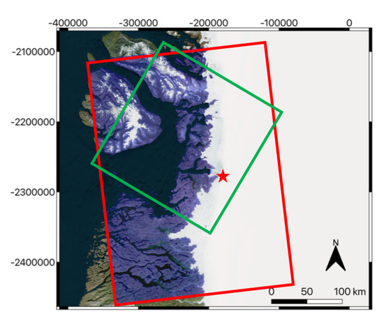
Figure 3.
Study area at the Jakobshavn Isbræ glacier, where the “red” rectangle marks the Sentinel-1 data coverage, the “green” rectangle marks the Landsat-8 coverage, the shaded “purple” area represents the stable surfaces used for comparison against the reference velocity map for error characterization and the “red” star marks the location over the fast-moving glacier outlet for the validation of the velocity estimates against high-resolution TanDEM-X data.

Table 1.
Sentinel-1 and Landsat-8 scenes utilized in this work.
To validate the accuracy of the velocity estimates, we performed two separate tests:
- (1)
- Stable surfaces (stationary or slow-flowing ice surface m/year, shown as the shaded “purple” area in Figure 3): We first extracted the reference velocity over stable surfaces and used the median absolute deviation (MAD) of the residual to characterize the displacement accuracy. Since the surface velocities for areas of “stable” flow experience negligible temporal variability, we used the 20-year ice-sheet-wide velocity mosaic [37,38] derived from the synthesis of SAR/InSAR data and Landsat-8 optical imagery as the reference velocity map. Stable surfaces were identified as those areas with a velocity less than 15 m/year, which primarily consisted of rocks in our study area, as shown in Figure 3 as most ice in this area flows at a rate greater than 15 m/year.
- (2)
- To characterize errors for the fast-flowing glacier outlet (N , W ; marked as the “red” star in Figure 3), we used dense time series of SAR/InSAR-derived velocity estimates [38,39] from TanDEM-X mission as the truth dataset and calculated the difference (relative percentage) relative to estimates generated using autoRIFT.
Due to the large interannual and seasonal velocity variation of the Jakobshavn Isbræ glacier [40], we relied on the accuracy metrics derived from the analysis over stable surface to characterize displacement errors.
As tabulated in Table 1, 11 Sentinel-1A/B images and 10 Landsat-8 images, all acquired in 2017 over the Jakobshavn Isbræ glacier, were selected to validate our feature tracking routine. These data were selected to provide one image pair in each quarter throughout the year of 2017, as well as one image pair for each temporal baseline (time separation of the two images). Feature tracking results were generated for the seven Sentinel-1 and seven Landsat-8 image pairs listed in Table 2. To map radar viewing geometry, we used the GIMP DEM [41,42] for the Greenland Ice Sheet. Both the DEM and the reference velocity map were further resampled to a grid with 240 m spacing and a spatial reference system of EPSG code 3413 (WGS 84 / NSIDC Sea Ice Polar Stereographic North).
Table 2.
Pairs of Sentinel-1 and Landsat-8 scenes in Table 1 for the validation of the velocity estimates with error metrics. ROI: region of interest.
3.2. Data Processing
Both autoRIFT and Geogrid have been integrated into the InSAR Scientific Computing Environment (ISCE (https://github.com/isce-framework/isce2) (accessed on 10 January 2021)) to support both Cartesian and radar coordinates and can also be used as a standalone Python module (https://github.com/conda-forge/autorift-feedstock (accessed on 10 January 2021)) that only supports Cartesian coordinates.
Before performing feature tracking, the two images for each pair in Table 2 needed to be co-registered. The Sentinel-1 Level 1.1 Interferometric Wide (IW) swath mode Single Look Complex (SLC) radar images were pre-processed using the ISCE software. The Geogrid module was then run for each image pair to determine the mapping between image coordinates and geographic coordinates, where the geographic coordinates were defined by an input grid. The input grid can be a real DEM when using radar coordinates (as required for mapping of radar viewing geometry) or a “blank” DEM (all zero values) for Cartesian coordinates. There were also a few other optional inputs; e.g., local surface slopes by taking the gradients of DEM, a reference velocity for downstream search, reference velocity-based search distance (in m/year) and minimum and maximum bounds of window size (in m), all of which could be spatially varying for both X-/Y-direction components and shared the same geographic grid (with a 240 m grid spacing and the projection of Polar Stereographic North in this work).
Two outputs of Geogrid are shown in Figure 4. The radar range-direction downstream search pixel displacement is shown in Figure 4a, which was calculated from the optional input of the downstream search reference velocity. Further, the range-direction search distance (in pixels) is shown in Figure 4b, which was calculated from the optional input of the reference velocity-based search distance (in m/year). Note that the second look-up table in Section 2.2 was used for generating both outputs in image coordinates (i.e., range/azimuth pixel displacement) from the optional inputs in geographic coordinates (i.e., X-/Y-direction reference velocity). The first look-up table between range/azimuth pixel index and geolocation is illustrated by the two “red" arrows in Figure 4.
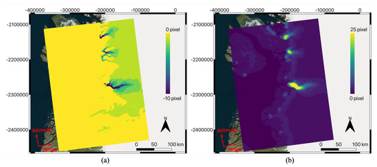
Figure 4.
Output of Geogrid module for Sentinel-1 data on a reference geographic grid (NSIDC North Polar Stereographic): (a) range pixel displacement for downstream search, (b) range search distance. Both outputs were calculated using the 2nd look-up table above. The colorbar unit shows the pixels in both of the subfigures. Note that the 1st look-up table between pixel index and geolocation is not displayed but shown by the two “red” arrows.
Using the Geogrid module outputs as inputs to the autoRIFT module, we obtained the final feature tracking outputs illustrated in Figure 5 for the Sentinel-1 and Landsat-8 image pairs with the highest ROI coverage in Table 2. Given the grid spacing of 240 m in the geographic grid and the pixel size for each type of sensor (4 m/15 m in range/azimuth for Sentinel-1 and 15 m in both dimensions for Landsat-8), to maintain template independence, we used progressive chip sizes from 32 to 64 for Sentinel-1 image pairs and from 16 to 32 for Landsat-8 image pairs. An NCC correlation surface oversampling ratio of 64 was used for all of the image pairs so that the sub-pixel program could be solved to the precision of 1/64 pixel. All of the variables are output on the same geographic grid as the input DEM to Geogrid.
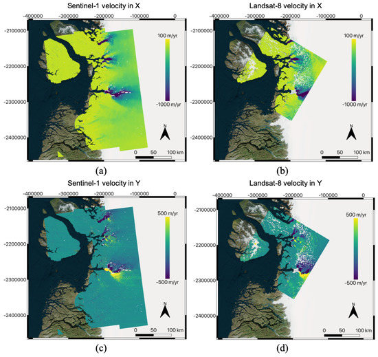
Figure 5.
Velocity output of the autoRIFT module for the Sentinel-1 pair and the Landsat-8 pair with the best coverage in this work: (a) Sentinel-1 velocity in X direction, (b) Landsat-8 velocity in X direction, (c) Sentinel-1 velocity in Y direction, (d) Landsat-8 velocity in Y direction. The colorbar unit is in m/year in all of the subfigures. The Sentinel-1 pair is 20170404–20170410, and the Landsat-8 pair is 20170718–20170803, as identified in Table 2 with the highest ROI coverage.
From Figure 5, the radar and optical results can be seen to compare well with one another, except for the streak artifacts in radar azimuth direction which are noticeable in the geographic Y direction (Figure 5c). Note that the Sentinel-1 dataset was acquired in ascending orbits with the azimuth component predominantly affecting the geographic Y direction. The streak artifacts in Figure 5c are random and due to the ionosphere effects [4,19,21,23,24,43] in the radar azimuth direction that can be minimized by stacking/averaging multiple observations.
3.3. Error Characterization
As outlined in Section 3.1, the velocity errors over the stable surfaces (stationary—e.g., rock—or slow-flowing ice surfaces with a reference velocity <15 m/year, as illustrated in Figure 3) were calculated for each image pair and are tabulated in Table 2. The error metrics are provided in geographic X/Y directions, and in range/azimuth for radar imagery.
Before calculating the error metric (MAD), the reference velocity needed to be subtracted over stable surfaces and the residual velocity median bias needed to be taken out. Satellite optical imagery can suffer from large (5 to 30 m) mean geolocation errors that manifest as large shifts in displacement [34]. These can be easily corrected for by applying median bias adjustments as determined through a comparison with stable surfaces. The correction for the median displacement error was also performed for the radar results (Table 2), although this error is usually negligible for radar imagery.
For the four radar image pairs with a temporal baseline of 6 days (one pair in each quarter), the velocity errors, as well as the region of interest (ROI) coverage, exhibited noticeable seasonal effects. The errors in January and October were almost twice as large as those in April and July, which implies that the accuracy of winter acquisitions can be worse, with a loss of correlation likely due to changes in surface properties; e.g., heavy snowfall and/or change in water content. The ROI coverage in July (43%) was lower compared to other times of year (>85%), which can be explained by the strong temporal decorrelation due to surface melting. Among all Sentinel-1 pairs, the April pair had the best spatial coverage (an ROI coverage of 100%) and accuracy (with errors of 12 m/year in X and 39 m/year in Y). The corresponding errors in radar coordinates were 8 m/year in range and 44 m/year in azimuth. Errors in the azimuth direction were much larger than in the range direction because of increased sensitivity to ionospheric delays and four times coarser spatial resolution (see Table 1). The velocity magnitude error for this 6 day Sentinel-1A/B pair was 22 m/year, which was within the range of the reported values (17–25 m/year) from 12 day Sentinel-1A pairs over the slow-moving areas in Greenland [44].
We next examined the temporal baseline dependence of the radar-measured error metrics. Four temporal baselines (6, 12, 18 and 24 days) were selected as in Table 2 with reference to the best pair in April. The ROI coverage dropped slowly from 100% to 60%, and the errors did not change remarkably, with some being slightly better than the 6 day pair. Note that this result itself (with only one sample for each temporal baseline) was not sufficient to conclude that the velocity errors did not drop as the temporal baseline increased; rather, it may imply that the decrease rate of velocity error was not very large. Larger temporal baselines (e.g., greater than 36 days) usually cause severe temporal decorrelation (thus, small ROI coverage) in Sentinel-1 image pairs.
For the four optical image pairs at the temporal baseline of 16 days (one pair in each quarter, and the October pair was only available with 32 days), both the velocity errors and the ROI coverage exhibited strong seasonal effects. The pair with the largest velocity errors was in January (91 m/year in X and 160 m/year in Y) due to low illumination and poor surface contrast during the polar night. The pair with the lowest errors was in July (22 m/year in X and 31 m/year in Y) when ROI coverage peaked at 84%. This July coverage maxima was opposite to the July coverage minima for the radar results, implying that both the optical and radar satellite imagery complement each other when mapping polar ice sheet motion. It should be noted that the presence of cloud greatly affects the ROI coverage when using optical imagery.
An analysis of temporal baseline dependence was performed for the optical error metrics. Four temporal baselines (16, 32, 64 and 368 days) were selected as shown in Table 2. The ROI coverage became very low at 32 day and 64 day temporal baselines due to the presence of a large amount of cloud cover, while the accuracy was not substantially impacted. However, with a 368 day temporal baseline, the errors dropped by a factor of 10–15 while the ROI coverage was 10% better than the 64 day case. This is a big advantage of using optical satellite imagery with long temporal baselines (of a few months to a year) as radar imagery decorrelates at such long temporal baselines (i.e., a year).
All of the error metrics reported in this work are specific to the used Sentinel-1A/B and Landsat-8 image pairs over the Jakobshavn Isbræ test site with the current processing setup (a progressive chip size with minimum/maximum of 32/64 for radar and 16/32 for optical processing, as well as a sub-pixel oversampling ratio of 64). Besides seasonal variation and time separation dependence, errors and ROI coverage are expected to change greatly between image pairs depending on environmental factors such as local surface conditions, illumination, cloud cover, ionosphere disturbance, feature persistence and surface deformation.
3.4. Validation with TanDEM-X Time Series
As outlined in Section 3.1, the velocity estimates over fast-flowing ice surfaces (Jakobshavn Isbræ glacier outlet, marked as the “red” star in Figure 3) were compared with dense time series of SAR/InSAR-derived velocity estimates [38,39] from TanDEM-X data (ground truth). We calculated the difference (relative percentage) between the ground truth and the estimates (also tabulated in Table 2).
Although the ground truth data are generally derived using the combined method of feature tracking (over fast-moving ice) as well as SAR interferometry (over slow-flowing ice) [38], in our test site, they were primarily derived from TerraSAR-X data using the feature tracking method and were only available for the area covering the terminus of the Jakobshavn Isbræ glacier near the “red” star in Figure 3. The time-series results are illustrated in Figure 6, where the TanDEM-X results were available for almost every 5 days during the majority of the year. There was a remarkable seasonal variability in velocity at this fast-flowing glacier outlet, where the X and Y-direction velocities were anticorrelated.
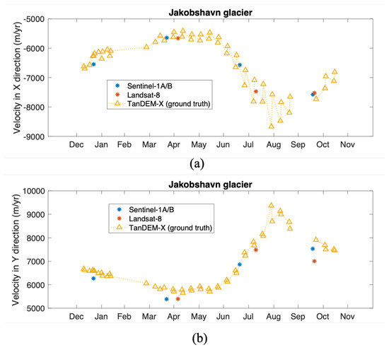
Figure 6.
Comparison of the velocity time-series estimates of the Sentinel-1 and Landsat-8 data in this work against the ground-truth data (TanDEM-X) over the fast-moving glacier outlet as marked in Figure 3: (a) velocity in X direction, (b) velocity in Y direction.
To compare with the ground truth, we selected one image pair in each quarter from both Sentinel-1 and Landsat-8 datasets. The pixel value of the Landsat pair in January was not available for this location due to the polar darkness. As tabulated in Table 2, the difference for Sentinel-1 data was roughly 250 m/year with a relative percentage of 4% for both X and Y-directions and did not show a noticeable seasonal variation. Note the velocity fluctuation in the ground truth time series that is prominent between June and September was likely an artifact of changing the TanDEM-X acquisition geometry.
From Table 2, the X and Y-direction velocity estimates from Landsat-8 data can be observed to be slightly different compared to the ground truth: 200 m/year with a relative percentage of 3% for X-direction and 500 m/year with a relative percentage of 7% for the Y-direction, where the velocity difference does not show a noticeable seasonal variation. The large difference in X and Y-direction velocity errors could be due to the orientation of linear crevasse features, a strong velocity gradient, differing sensor viewing geometry or errors in the DEM used in either the TanDEM-X or Landsat processing. The current study site at the terminus of the Jakobshavn Isbræ glacier serves as the worst-case example (maximum errors expected) as it is the fastest glacier in the world (rapid decorrelation), is experiencing extreme rates of thinning (up to 50 m/year) and has strong spatial gradients and large inter-annual variability.
As shown in Table 2, the difference between our estimates from Sentinel-1 A/B or Landsat-8 and the ground truth TanDEM-X data could be much larger than the error metrics reported in Section 3.3, with large spatial and temporal variability at fast-moving glacier outlets. This has been confirmed with other studies [44,45] that showed that velocity estimates derived from Sentinel-1 and TanDEM-X have a good agreement over most parts of Greenland; however, the difference can be as large as 4–8% in areas with strong spatial gradients in surface velocity (e.g., our study site in this section). Therefore, the velocity difference at the fast-moving glacier outlet does not characterize the overall error in the velocity retrieval well; rather, the reported disagreement represents a combination of differing sensor resolution, temporal variability in surface flow, error in TanDEM-X velocities and errors in autoRIFT-derived velocities.
3.5. Runtime and Accuracy Comparison
In this section, we compare the runtime and accuracy between ampcor and autoRIFT. As shown in Table 3, the advanced version of ampcor (“dense ampcor"; with a much denser grid) from the ISCE software (v2.2.0) was used for comparison with multiple modes of autoRIFT. Since dense ampcor only supports radar images and image grids (not geographic grids), we first performed an apples-to-apples comparison between dense ampcor and the standard mode of autoRIFT in the image grid (range/azimuth coordinates) for one Sentinel-1A/B image pair (20170221–20170227) in Table 1.
Table 3.
Runtime and accuracy comparison between the conventional dense ampcor and the proposed autoRIFT algorithms. Scenario ➀: smaller window size, scenario ➁: bigger window size, scenario ➂: progressive window size from ➀ to ➁.
As shown in the first two columns of Table 3, two different window (chip) sizes were selected: 32 (defined as Scenario ➀) and 64 (defined as Scenario ➁), where autoRIFT also ran with a progressive chip size from 32 to 64 (defined as Scenario ➂ where results from both chip sizes were obtained and fused). The spacing of the search grid was correspondingly adjusted from 32 to 64.
Without the help of a downstream search routine, a very large search distance is required for fast-flowing ice surfaces, especially for the current test site. From recent studies, the maximum velocity of the Jakobshaven glaciers has been found to be around 15 km/year, with an overall seasonal range of 8 km/year [40]. We therefore used a search range of pixels in range and pixels in azimuth. An oversampling ratio of 64 was used for the sub-pixel program.
Dense ampcor requires the two radar images to be pre-processed by ISCE so that they are co-registered SLC images. Similarly, autoRIFT also assumes the two images are co-registered and has the option of high-pass filtering with various kernels (e.g., a normalized/unnormalized Wallis filter) as well as converting to different data types (e.g., an 8-bit unsigned integer or 32-bit single-precision float). Dense ampcor (written using Fortran) uses eight threads, while autoRIFT (written using Python and C++) uses a single thread despite the fact that it has been parallelized with the capability of multithreading. Although dense ampcor has the capability of performing complex-valued NCC, it has been primarily used for offset tracking between the SAR amplitude images.
Using the same search grid, search distance and chip size, autoRIFT’s runtime was found to be 6.4 min/core compared to ampcor’s 480.0 min/core for Scenario ➀ and 2.6 min/core compared to ampcor’s 368.0 min/core (141 times) for Scenario ➁. Under Scenario ➂, autoRIFT’s runtime was slightly smaller than the sum of the above two scenarios. On average, autoRIFT exhibited two orders of magnitude runtime improvement compared to dense ampcor. Note that the runtime metrics reported in this work are specific to an OS X operating system with 2.9GHz Intel Core i7 processor (with eight cores available) and 16 GB RAM.
Range (i) and azimuth (j) displacement errors are also compared in Table 3. For our test image pair, autoRIFT is shown to provide a ∼20% improvement in accuracy (MAD: 0.007-0.008 pixel) over dense ampcor. Similar to Section 3.3, these error metrics were calculated over stable surfaces (the shaded “purple" region in Figure 3). Since dense ampcor does not employ any filtering to remove bad matches, we calculated the error of dense ampcor results wherever autoRIFT produced reliable estimates. Our results show that autoRIFT greatly improves the runtime without sacrificing accuracy. Improvements result from the implementation of advanced techniques (e.g., a sparse/dense combinative search strategy as well as Gaussian pyramid upsampling algorithm for the sub-pixel program and the adaptive NDC filter as detailed in Section 2.1) that are shown to improve both the computational efficiency and accuracy. The accuracy of autoRIFT for Scenario ➂ (with progressive window size from 32 to 64) is mostly governed by the results with a smaller window size (i.e., 32 as used in Scenario ➀).
We also show results for autoRIFT’s Scenario ➂ which ran with regular-spaced search centers on a 240 m geographic grid (the 3rd column in Table 3), instead of the regular-spaced image grids used in the previous example. Runtime and accuracy are comparable to those of the run with regular-spaced image grid search centers, where the accuracy in azimuth (j) direction improved slightly (by 0.008 pixel).
autoRIFT can also be run in the intelligent mode (Note in this work, the word “intelligent” does not mean artificial intelligence and/or machine learning types of approaches; rather, it specifically means the use of various spatially-varying inputs) using various inputs as described in Section 2.1 and Section 3.2 for further improved computational efficiency. The first intelligent use (the 4th column in Table 3) was to incorporate a downstream search routine, where a spatially varying downstream search pixel displacement is provided, as illustrated in Figure 4a. The runtime further improved by 1.4 min/core with an accuracy comparable to the standard mode. The second intelligent use (the 5th column in Table 3) was to further include a spatially varying search distance in range direction (as illustrated in Figure 4b) along with the downstream search routine. The runtime further improved by 0.6 min/core and produced comparable accuracy results.
With standard autoRIFT, we observed more than two orders of magnitude runtime improvement, while the intelligent use of autoRIFT further enhanced the efficiency. This test case was for a short time-separation image-pair, and further time improvement over conventional techniques would be achieved as the time-separation between image-pairs increased; i.e., the expected displacements would increase and therefore the search distance would need to be increased without the implantation of a downstream search routine.
4. Discussion
With the nested grid design, sparse/dense combinative search strategy, adaptive sub-pixel estimation and the disparity filtering technique (the NDC filter), autoRIFT remarkably improves computational efficiency by estimating the displacements with an iteratively progressive chip size and by separating signal from noise. This standard use of autoRIFT has more than two orders of magnitude runtime improvement over a conventional NCC-based feature tracking routine (dense ampcor). In addition, autoRIFT is able to extract more information from the image pair and identify signal from noise without compromising the accuracy of the solution.
Importantly, autoRIFT can also run in the intelligent mode by specifying the downstream search displacement, search distance and minimum and maximum progressive chip size, all of which can vary spatially to accommodate regions with differing flow characteristics. A zero search distance can be assigned to areas of the image in which displacement estimates are not needed. The oversampling ratio in a sub-pixel program can also be adaptively selected as a function of chip size. For example, NCC results with a low signal to noise ratio (SNR) (e.g., a small chip size, relatively high image noise, low texture, etc.) will not benefit from higher oversample ratios that can be computationally costly, i.e., small oversampling ratios (e.g., 16 or 32) are sufficient. NCC results with high SNR (e.g., large chip size) are more suitable for a high oversample the ratio (e.g., 64 or 128) that needs to be selected as a tradeoff between precision and efficiency. This intelligent use of autoRIFT further improves the runtime, especially over areas with fine spatial sampling and also a large magnitude and variability of velocity.
In combination with Geogrid, autoRIFT can run on any user-defined geographic grid. NCC is still performed in the native image coordinates (e.g., radar coordinates for radar image pairs and geographic Cartesian coordinates for optical image pairs), and the displacement results are directly assigned to a geographic grid without interpolation/resampling. This approach ensures that no information is lost in the resampling of the imagery or resulting displacement fields.
Two look-up tables are created by the Geogrid module: one for mapping from the pixel index in the image to the geolocation on the geographic grid and the other for mapping from pixel displacement in the image to the velocity on the geographic grid. As long as a geographic grid is provided, the Geogrid module can map between the image coordinates (pixel index and displacement) and the geographic coordinates (geolocation and velocity). For example, the second look-up table maps the reference velocity (geographic) to downstream search pixel displacement (image) and, inversely, the estimated pixel displacement (image) to velocity (geographic).
The accuracy of the velocity estimates vary seasonally and depend on a number of factors such as ionosphere disturbance and temporal decorrelation for radar image pairs and polar darkness/cloud presence for optical image pairs. The accuracy and ROI coverage of the displacement results further depend on the quality of the source imagery, search chip size, surface texture, time separation, sub-pixel oversampling ratio, local surface conditions, illumination, cloud cover, ionosphere disturbance, feature persistence and surface deformation. For radar images, azimuth (j-direction) streaks, due to ionosphere effects, can be minimized by stacking/averaging results from multiple image pairs. The displacement error in the radar azimuth direction is larger due to the increased sensitivity to ionospheric delay and larger azimuth pixel resolution for the Sentinel-1 mission and can be partially mitigated by using search chips with a larger chip height (j-direction) than chip width (i-direction). For optical images, the displacement errors in both directions are comparable.
5. Conclusions
This paper describes the design and application of a feature tracking routine that is comprised of a feature tracking module (autoRIFT; first presented in [34]) and a novel geocoding module (Geogrid). The routine supports feature tracking at both image and geographic grids and supports both radar and optical imagery.
autoRIFT has been validated with seven Sentinel-1A/B radar image pairs and seven Landsat-8 optical image pairs in 2017 over the Jakobshavn Isbræ glacier. Errors of velocity estimates are characterized over stable surfaces for the test site. The Sentinel-1A/B image pair with the highest ROI coverage and lowest error was found to be in April, 2017 with an error in geographic X/Y directions of 12 m/year or 39 m/year and error in slant-range/azimuth of 8 m/year or 44 m/year. The Landsat-8 image pair with the highest ROI coverage and lowest error was in July, 2017 complementing the radar observations with an error in geographic X/Y directions of 22 m/year or 31 m/year.
An analysis of temporal baseline dependence was also performed. For the Sentinel-1 imagery, we tested temporal baselines of 6, 12, 18 and 24 days; the error metrics did not change significantly as the temporal baseline increased, but ROI coverage dropped from 100% to 60%. For Landsat-8 image pairs, we tested temporal baselines of 16, 32, 64 and 368 days, where the 32 day and 64 day results were mostly affected by the presence of cloud cover. Unlike the temporal decorrelation problem dominating radar image pairs, a temporal baseline of a year (368 days) was found to remarkably improve the accuracy of results derived from optical imagery (by a factor of 10–15) while maintaining high ROI coverage (48%).
Velocity estimates were also compared with the reference velocity derived from TanDEM-X data over the fast-moving glacier outlet, where the ice velocity showed strong seasonal variability. The results from Sentinel-1 had a relative error of 4% on average for both X and Y-direction velocity, and those from Landsat-8 had a relative error of 3–7% (with a slightly larger difference for Y-direction velocity). There was no noticeable seasonal variation in the disagreement with TanDEM-X derived velocities.
We performed an apples-to-apples comparison of runtime and accuracy between a conventional open-source NCC-based feature tracking software, dense ampcor, from NASA/JPL’s ISCE software, and multiple modes of autoRIFT. For each mode of autoRIFT, more than two orders of magnitude runtime improvement along with a 20% improvement in accuracy was achieved relative to dense ampcor. Further, the intelligent uses of autoRIFT by incorporating a spatially-varying downstream search routine and/or search distance further improved the computational efficiency.
A standalone version of autoRIFT is already being used to generate global land ice displacement velocities from the full archive of Landsat 4/5/7 and 8 imagery as part of the NASA MEaSUReS ITS_LIVE initiative (https://its-live.jpl.nasa.gov/ accessed on 10 January 2021). Its integration into the ISCE radar processing software and inclusion of the new Geogrid module now allow for the global mapping of ice displacement from both optical and radar imagery using a single algorithm on identical output grids. The orders of magnitude reduction in computational cost demonstrated with the new algorithms is particularly relevant for NASA’s upcoming NISAR mission, which will downlink more data than any prior mission. Future efforts will expand the current capabilities to include complex-valued NCC (using both amplitude and phase in SAR SLC images).
Author Contributions
Conceptualization, Y.L., A.G. and P.A.; methodology, Y.L., A.G. and P.A.; software, Y.L., A.G. and P.A.; validation, Y.L.; analysis, Y.L.; writing—original draft preparation, Y.L.; writing—review and editing, A.G.; funding acquisition, A.G. All authors have read and agreed to the published version of the manuscript.
Funding
This effort was funded by the NASA MEaSUREs program in contribution to the Inter-Mission Time Series of Land Ice Velocity and Elevation (ITS_LIVE) project (https://its-live.jpl.nasa.gov/ (accessed on 10 January 2021)) and through Alex Gardner’s participation in the NASA NISAR Science Team. Research conducted at the Jet Propulsion Laboratory, California Institute of Technology under contract with the National Aeronautics and Space Administration.
Institutional Review Board Statement
Not applicable.
Informed Consent Statement
Not applicable.
Conflicts of Interest
The authors declare no conflict of interest.
Appendix A. Derivation of the Conversion Matrix
In this appendix, we derive the conversion matrix in (4) that converts the pixel displacements ( and ) to the velocity ( and ). Note that and are in dimensionless pixel units.
By substituting
where , , and , we have (1)–(3) rewritten as
By taking (A5) multiplied by minus (A7) multiplied by , the Z-terms are cancelled out, which leads to
where the coefficients are
Similarly, by taking (A6) multiplied by minus (A7) multiplied by , we have
where the coefficients are
Rearranging (A8) and (A12) gives the explicit form of (4); i.e.,
By inverting the matrix of (A16), we have
which concludes the derivation of the conversion matrix as defined in (4); i.e.,
The coefficients in (A18) are defined in (A9)–(A11) and (A13)–(A15), where components of and are derived from the second look-up table in the Geogrid module (Section 2.2), and components of are associated with the input surface slopes (derived from DEM) as mentioned above.
From (A18), it is known that the conversion matrix is undefined when the denominator . This could be the case for radar viewing geometry when the surface normal and the radar range-direction unit vector are co-aligned (i.e., by satisfying the vector relation, or ) for large surface slopes facing toward the radar over mountainous areas. The coefficients in (A9) and (A10) and (A13) and (A14) can be rewritten as X or Y-components (with notation or ) of vector cross products; i.e.,
Therefore, when is in line with , , meaning , thus . Note when this vector relation holds, the pixels must be masked out; otherwise, the converted displacement results will be unreliable.
Appendix B. Error Propagation due to the Failure of Slope Parallel Assumption
Here, we derive the horizontal velocity error (in both X and Y directions) induced by the deviation of the vertical velocity component from that estimated using the slope parallel assumption. In the following derivations, we use the notation without prime for slope parallel-estimated velocity results (as in Appendix A), and use the prime notation for the actual velocities.
Let us assume there is some error in the slope parallel-estimated vertical velocity component . The actual vertical velocity component, , can thus be rewritten as
where is the error due to slope parallel assumption. Thus, we would like to derive the propagated error of horizontal velocities in X and Y directions, and , by using the slope parallel assumption; i.e.,
Similar to Appendix A, (A5) and (A6) still hold for the prime notation by replacing the unprimed notation with the prime notation. However, (A7) needs to be modified as below:
Using (A26) along with the prime version of (A5) and (A6), we can follow exactly the same procedure in Appendix A to achieve the following results; i.e.,
By subtracting (A16) from (A27) and utilizing (A24) and (A25), we have
Through inverting the matrix of (A28), we have
where
Therefore, the error propagation is linear. After rearranging terms, (A30) and (A31) can be further simplified as components of vector cross products; i.e.,
From (A32) and (A33), it can be seen that the propagated error in X and Y directions can differ depending on the projection of the cross-product vector, , onto each of the two directions, which further depends on the sensor viewing geometry and/or terrain elevation.
For radar image pairs, since is the cross product of the unit vectors in the slant-range direction and azimuth direction, the vector cross product lies in the plane formulated by the radar range and surface normal vectors for a flat terrain. Therefore, the propagated error in X (or Y) direction is proportional to the projection of the radar range direction onto the X (or Y) direction. Using the Seninel-1 radar dataset of this work over the current test site, the radar range direction is closer to the X direction (see Figure 4); thus, a larger propagated error in X () is expected compared to that in Y ().
For optical image pairs, the vector cross product is simply equal to the surface normal. Therefore, , and thus , meaning there is no error propagation due to the failure of slope parallel assumption.
References
- Bindschadler, R.; Scambos, T. Satellite-image-derived velocity field of an Antarctic ice stream. Science 1991, 252, 242–246. [Google Scholar] [CrossRef] [PubMed]
- Frolich, R.; Doake, C. Synthetic aperture radar interferometry over Rutford Ice Stream and Carlson Inlet, Antarctica. J. Glaciol. 1998, 44, 77–92. [Google Scholar] [CrossRef][Green Version]
- Fahnestock, M.; Scambos, T.; Moon, T.; Gardner, A.; Haran, T.; Klinger, M. Rapid large-area mapping of ice flow using Landsat 8. Remote. Sens. Environ. 2016, 185, 84–94. [Google Scholar] [CrossRef]
- Strozzi, T.; Kouraev, A.; Wiesmann, A.; Wegmüller, U.; Sharov, A.; Werner, C. Estimation of Arctic glacier motion with satellite L-band SAR data. Remote. Sens. Environ. 2008, 112, 636–645. [Google Scholar] [CrossRef]
- Fahnestock, M.; Bindschadler, R.; Kwok, R.; Jezek, K. Greenland ice sheet surface properties and ice dynamics from ERS-1 SAR imagery. Science 1993, 262, 1530–1534. [Google Scholar] [CrossRef] [PubMed]
- Strozzi, T.; Luckman, A.; Murray, T.; Wegmuller, U.; Werner, C.L. Glacier motion estimation using SAR offset-tracking procedures. IEEE Trans. Geosci. Remote. Sens. 2002, 40, 2384–2391. [Google Scholar] [CrossRef]
- de Lange, R.; Luckman, A.; Murray, T. Improvement of satellite radar feature tracking for ice velocity derivation by spatial frequency filtering. IEEE Trans. Geosci. Remote Sens. 2007, 45, 2309–2318. [Google Scholar] [CrossRef]
- Nagler, T.; Rott, H.; Hetzenecker, M.; Scharrer, K.; Magnússon, E.; Floricioiu, D.; Notarnicola, C. Retrieval of 3D-glacier movement by high resolution X-band SAR data. In Proceedings of the 2012 IEEE International Geoscience and Remote Sensing Symposium, Munich, Germany, 22–27 July 2012; pp. 3233–3236. [Google Scholar]
- Kusk, A.; Boncori, J.P.M.; Dall, J. An automated system for ice velocity measurement from SAR. In Proceedings of the EUSAR 2018, 12th European Conference on Synthetic Aperture Radar, Aachen, Germany, 4–7 June 2018; pp. 1–4. [Google Scholar]
- Mouginot, J.; Rignot, E.; Scheuchl, B.; Millan, R. Comprehensive annual ice sheet velocity mapping using Landsat-8, Sentinel-1, and RADARSAT-2 data. Remote. Sens. 2017, 9, 364. [Google Scholar] [CrossRef]
- Riveros, N.C.; Euillades, L.D.; Euillades, P.A.; Moreiras, S.M.; Balbarani, S. Offset tracking procedure applied to high resolution SAR data on Viedma Glacier, Patagonian Andes, Argentina. Adv. Geosci. 2013, 35, 7–13. [Google Scholar] [CrossRef]
- Gourmelen, N.; Kim, S.; Shepherd, A.; Park, J.; Sundal, A.; Björnsson, H.; Pálsson, F. Ice velocity determined using conventional and multiple-aperture InSAR. Earth Planet. Sci. Lett. 2011, 307, 156–160. [Google Scholar] [CrossRef]
- Joughin, I.R.; Winebrenner, D.P.; Fahnestock, M.A. Observations of ice-sheet motion in Greenland using satellite radar interferometry. Geophys. Res. Lett. 1995, 22, 571–574. [Google Scholar] [CrossRef]
- Yu, J.; Liu, H.; Jezek, K.C.; Warner, R.C.; Wen, J. Analysis of velocity field, mass balance, and basal melt of the Lambert Glacier–Amery Ice Shelf system by incorporating Radarsat SAR interferometry and ICESat laser altimetry measurements. J. Geophys. Res. Solid Earth 2010, 115. [Google Scholar] [CrossRef]
- Mouginot, J.; Rignot, E.; Scheuchl, B. Continent-Wide, Interferometric SAR Phase, Mapping of Antarctic Ice Velocity. Geophys. Res. Lett. 2019, 46, 9710–9718. [Google Scholar] [CrossRef]
- Rignot, E.; Jezek, K.; Sohn, H.G. Ice flow dynamics of the Greenland ice sheet from SAR interferometry. Geophys. Res. Lett. 1995, 22, 575–578. [Google Scholar] [CrossRef]
- Gray, A.; Mattar, K.; Vachon, P.; Bindschadler, R.; Jezek, K.; Forster, R.; Crawford, J. InSAR results from the RADARSAT Antarctic Mapping Mission data: Estimation of glacier motion using a simple registration procedure. Proceedins of the 1998 IEEE International Geoscience and Remote Sensing, Seattle, WA, USA, 6–10 July 1998; Volume 3, pp. 1638–1640. [Google Scholar]
- Michel, R.; Rignot, E. Flow of Glaciar Moreno, Argentina, from repeat-pass Shuttle Imaging Radar images: Comparison of the phase correlation method with radar interferometry. J. Glaciol. 1999, 45, 93–100. [Google Scholar] [CrossRef]
- Joughin, I.R.; Kwok, R.; Fahnestock, M.A. Interferometric estimation of three-dimensional ice-flow using ascending and descending passes. IEEE Trans. Geosci. Remote Sens. 1998, 36, 25–37. [Google Scholar] [CrossRef]
- Joughin, I.; Gray, L.; Bindschadler, R.; Price, S.; Morse, D.; Hulbe, C.; Mattar, K.; Werner, C. Tributaries of West Antarctic ice streams revealed by RADARSAT interferometry. Science 1999, 286, 283–286. [Google Scholar] [CrossRef] [PubMed]
- Joughin, I. Ice-sheet velocity mapping: A combined interferometric and speckle-tracking approach. Ann. Glaciol. 2002, 34, 195–201. [Google Scholar] [CrossRef]
- Liu, H.; Zhao, Z.; Jezek, K.C. Synergistic fusion of interferometric and speckle-tracking methods for deriving surface velocity from interferometric SAR data. IEEE Geosci. Remote Sens. Lett. 2007, 4, 102–106. [Google Scholar] [CrossRef]
- Sánchez-Gámez, P.; Navarro, F.J. Glacier surface velocity retrieval using D-InSAR and offset tracking techniques applied to ascending and descending passes of Sentinel-1 data for southern Ellesmere ice caps, Canadian Arctic. Remote Sens. 2017, 9, 442. [Google Scholar] [CrossRef]
- Joughin, I.; Smith, B.E.; Howat, I.M. A complete map of Greenland ice velocity derived from satellite data collected over 20 years. J. Glaciol. 2018, 64, 1–11. [Google Scholar] [CrossRef] [PubMed]
- Merryman Boncori, J.P.; Langer Andersen, M.; Dall, J.; Kusk, A.; Kamstra, M.; Bech Andersen, S.; Bechor, N.; Bevan, S.; Bignami, C.; Gourmelen, N.; et al. Intercomparison and validation of SAR-based ice velocity measurement techniques within the Greenland Ice Sheet CCI project. Remote Sens. 2018, 10, 929. [Google Scholar] [CrossRef]
- Rosen, P.A.; Hensley, S.; Peltzer, G.; Simons, M. Updated repeat orbit interferometry package released. Eos Trans. Am. Geophys. Union 2004, 85, 47. [Google Scholar] [CrossRef]
- Rosen, P.A.; Gurrola, E.M.; Agram, P.; Cohen, J.; Lavalle, M.; Riel, B.V.; Fattahi, H.; Aivazis, M.A.; Simons, M.; Buckley, S.M. The InSAR Scientific Computing Environment 3.0: A Flexible Framework for NISAR Operational and User-Led Science Processing. In Proceedings of the IGARSS 2018-2018 IEEE International Geoscience and Remote Sensing Symposium, Valencia, Spain, 22–27 July 2018; pp. 4897–4900. [Google Scholar]
- Willis, M.J.; Zheng, W.; Durkin, W.; Pritchard, M.E.; Ramage, J.M.; Dowdeswell, J.A.; Benham, T.J.; Bassford, R.P.; Stearns, L.A.; Glazovsky, A.; et al. Massive destabilization of an Arctic ice cap. Earth Planet. Sci. Lett. 2018, 502, 146–155. [Google Scholar] [CrossRef]
- Willis, M.J.; Melkonian, A.K.; Pritchard, M.E.; Ramage, J.M. Ice loss rates at the Northern Patagonian Icefield derived using a decade of satellite remote sensing. Remote. Sens. Environ. 2012, 117, 184–198. [Google Scholar] [CrossRef]
- Mouginot, J.; Scheuchl, B.; Rignot, E. Mapping of ice motion in Antarctica using synthetic-aperture radar data. Remote Sens. 2012, 4, 2753–2767. [Google Scholar] [CrossRef]
- Millan, R.; Mouginot, J.; Rabatel, A.; Jeong, S.; Cusicanqui, D.; Derkacheva, A.; Chekki, M. Mapping surface flow velocity of glaciers at regional scale using a multiple sensors approach. Remote Sens. 2019, 11, 2498. [Google Scholar] [CrossRef]
- Casu, F.; Manconi, A.; Pepe, A.; Lanari, R. Deformation time-series generation in areas characterized by large displacement dynamics: The SAR amplitude pixel-offset SBAS technique. IEEE Trans. Geosci. Remote. Sens. 2011, 49, 2752–2763. [Google Scholar] [CrossRef]
- Euillades, L.D.; Euillades, P.A.; Riveros, N.C.; Masiokas, M.H.; Ruiz, L.; Pitte, P.; Elefante, S.; Casu, F.; Balbarani, S. Detection of glaciers displacement time-series using SAR. Remote Sens. Environ. 2016, 184, 188–198. [Google Scholar] [CrossRef]
- Gardner, A.S.; Moholdt, G.; Scambos, T.; Fahnstock, M.; Ligtenberg, S.; van den Broeke, M.; Nilsson, J. Increased West Antarctic and unchanged East Antarctic ice discharge over the last 7 years. Cryosphere 2018, 12, 521–547. [Google Scholar] [CrossRef]
- Stein, A.N.; Huertas, A.; Matthies, L. Attenuating stereo pixel-locking via affine window adaptation. In Proceedings of the 2006 IEEE International Conference on Robotics and Automation, Orlando, FL, USA, 15–19 May 2006; pp. 914–921. [Google Scholar]
- Tsang, L.; Kong, J.A. Scattering of Electromagnetic Waves: Advanced Topics; John Wiley & Sons: Hoboken, NJ, USA, 2004; Volume 26. [Google Scholar]
- Joughin, I.; Smith, B.; Howat, I.; Scambos, T. MEaSUREs Multi-year Greenland Ice Sheet Velocity Mosaic, Version 1; NASA National Snow and Ice Data Center Distributed Active Archive Center: Boulder, CO, USA; Available online: https://doi.org/10.5067/QUA5Q9SVMSJG (accessed on 2 July 2020).
- Joughin, I.; Smith, B.E.; Howat, I.M.; Scambos, T.; Moon, T. Greenland flow variability from ice-sheet-wide velocity mapping. J. Glaciol. 2010, 56, 415–430. [Google Scholar] [CrossRef]
- Joughin, I.; Smith, B.; Howat, I.; Scambos, T. MEaSUREs Greenland Ice Velocity: Selected Glacier Site Velocity Maps from InSAR, Version 3; NASA National Snow and Ice Data Center Distributed Active Archive Center: Boulder, CO, USA; Available online: https://doi.org/10.5067/YXMJRME5OUNC (accessed on 2 July 2020).
- Lemos, A.; Shepherd, A.; McMillan, M.; Hogg, A.E.; Hatton, E.; Joughin, I. Ice velocity of Jakobshavn Isbræ, Petermann Glacier, Nioghalvfjerdsfjorden, and Zachariæ Isstrøm, 2015–2017, from Sentinel 1-a/b SAR imagery. Cryosphere 2018, 12, 2087–2097. [Google Scholar] [CrossRef]
- Howat, I.; Negrete, A.; Smith, B. MEaSUREs Greenland Ice Mapping Project (GIMP) Digital Elevation Model, Version 1; NASA National Snow and Ice Data Center Distributed Active Archive Center: Boulder, CO, USA; Available online: https://doi.org/10.5067/NV34YUIXLP9W (accessed on 2 July 2020).
- Howat, I.M.; Negrete, A.; Smith, B.E. The Greenland Ice Mapping Project (GIMP) land classification and surface elevation data sets. Cryosphere 2014, 8, 1509–1518. [Google Scholar] [CrossRef]
- Liao, H.; Meyer, F.J.; Scheuchl, B.; Mouginot, J.; Joughin, I.; Rignot, E. Ionospheric correction of InSAR data for accurate ice velocity measurement at polar regions. Remote. Sens. Environ. 2018, 209, 166–180. [Google Scholar] [CrossRef]
- Nagler, T.; Rott, H.; Hetzenecker, M.; Wuite, J.; Potin, P. The Sentinel-1 mission: New opportunities for ice sheet observations. Remote Sens. 2015, 7, 9371–9389. [Google Scholar] [CrossRef]
- Joughin, I.; Smith, B.E.; Howat, I. Greenland Ice Mapping Project: Ice Flow Velocity Variation at sub-monthly to decadal time scales. Cryosphere 2018, 12, 2211. [Google Scholar] [CrossRef] [PubMed]
Publisher’s Note: MDPI stays neutral with regard to jurisdictional claims in published maps and institutional affiliations. |
© 2021 by the authors. Licensee MDPI, Basel, Switzerland. This article is an open access article distributed under the terms and conditions of the Creative Commons Attribution (CC BY) license (http://creativecommons.org/licenses/by/4.0/).