Abstract
To cope with the increasingly complex electromagnetic environment, multistatic radar systems, especially the passive multistatic radar, are becoming a trend of future radar development due to their advantages in anti-electronic jam, anti-destruction properties, and no electromagnetic pollution. However, one problem with this multi-source network is that it brings a huge amount of information and leads to considerable computational load. Aiming at the problem, this paper introduces the idea of selecting external illuminators in the multistatic passive radar system. Its essence is to optimize the configuration of multistatic T/R pairs. Based on this, this paper respectively proposes two multi-source optimization algorithms from the perspective of resolution unit and resolution capability, the Covariance Matrix Fusion Method and Convex Hull Optimization Method, and then uses a Global Navigation Satellite System (GNSS) as an external illuminator to verify the algorithms. The experimental results show that the two optimization methods significantly improve the accuracy of multistatic positioning, and obtain a more reasonable use of system resources. To evaluate the algorithm performance under large number of transmitting/receiving stations, further simulation was conducted, in which a combination of the two algorithms were applied and the combined algorithm has shown its effectiveness in minimize the computational load and retain the target localization precision at the same time.
1. Introduction
With the rapid development of science and technology, the modern electromagnetic environment has become more complex and changeable. Although the monostatic radar is powerful, it has a single detection of perspective and obtains incomplete information, so it cannot fight against the complex electromagnetic environment [1]. In response to the complex situation, a number of new concepts and new radar systems have gradually emerged. Among them, multistatic radar system will be a trend of future radar development.
Currently, the widely studied multistatic radar systems [1,2,3] include the networked radar [4,5], bistatic (multistatic) radar [6,7], and distributed MIMO radar [8,9,10]. Compared with monostatic radar, multistatic radar has the following advantages [11,12,13]: (1) It can detect targets in multiple directions to facilitate target recognition and anti-stealth. (2) Each transmitter can have different frequency bands and data rates, so it is beneficial to enhance the anti-jamming capability and reliability of the system. (3) It can increase the target detection probability and improve the positioning accuracy. (4) The system’s survivability is stronger, because the local transmitting or receiving abnormality cannot cause the collapse of the entire system. At present, many relevant studies have been done on the multistatic radar [14,15,16,17,18], and they have also been successfully applied in the fields of strategic indication warning, navigation system, and air traffic control. The representative research results are the Russian barrier radar [19], Japan’s bistatic radar system for ground detection [6], and the passive detection and positioning system researched by the British Defense Research Agency [20].
For the multistatic radar, the use of external illuminators is also a mainstream trend. On the one hand, with the rapid development of technology, there are many types of external illuminators that can be used, such as navigation satellites, communication satellites, and various ground-based base stations. On the other hand, in the face of an increasingly complex electromagnetic environment, a passive radar has more obvious advantages than an active radar. All major countries are now developing the wide-area detection networks combining active and passive radars [21,22,23,24]. However, the wide-area detection network also has a problem, in that it brings a huge amount of information and requires considerable computing power. For active networks, there is a closed-loop problem of cognitive transmission and the intelligent processing of receiving signal. For example, the literature [25] focuses on the joint processing of cognitive transmission and reception. For passive networks, the problem of selecting external illuminators is introduced. In essence, both these problems can be transformed into modeling optimization problems of T/R pairs configuration and system parameters.
This paper aims at the selection of external illuminators in the multistatic radar system and uses GNSS as the external illuminator. At present, with the continuous improvement of GNSS, the GNSS-based radar has received widespread attention, and it also has the advantages of all-weather and global coverage, and no extra electromagnetic pollution from the active radar transmitter. Moreover, for an arbitrary point on Earth, there are more than 30 satellites illuminators at any time. Therefore, many related research works have been conducted on it, such as target detection [26,27,28], positioning [29,30], kinematic state estimation [31], imaging [32,33], etc. The work of this paper is based on the literature [26,27,29].
On the premise that the approximate location of the target is known, this paper proposes two multi-source optimization algorithms from the perspective of resolution unit and resolution capability: Covariance Matrix Fusion Method and Convex Hull Optimization Method, and then uses GNSS as an external illuminator to verify the algorithms. GNSS itself has the accurate positioning capability, so the design of the satellite constellation orbit is a better geometric configuration for multistatic positioning. On this basis, after adopting our algorithms, it can achieve more effective passive target positioning.
The remaining arrangements of this paper are as follows: Section 2 briefly explains positioning method of multistatic radar and analyzes the positioning performance. Section 3 introduces the two proposed optimization algorithms in detail. The experimental simulation results are provided in Section 4. Finally, a conclusion is given in Section 5.
2. Target Localization Scheme with Multistatic Radar
2.1. System Geometry and Positioning Method Description
As shown in Figure 1, a multistatic radar system is composed of more than one transmitter or receiver or both. A multistatic geometry containing transmitters and one receiver can be easily extended to multiple-receiver cases, with all proposed methods in this paper still effective.
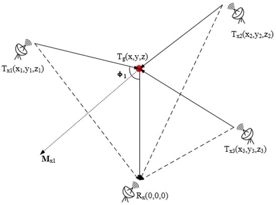
Figure 1.
Geometric structure of the multistatic radar system (for visibility, only three of bistatic T/R pairs are illustrated).
Without the loss of generality, it is assumed that the receiver is located at the coordinate origin (0,0,0). The positions of target and transmitters are defined as:
And
where .
The multistatic radar system can be regarded as bistatic T/R pairs. For visibility, only three of bistatic T/R pairs are illustrated in Figure 1. is the bistatic angle of the bistatic radar. is the bistatic angle bisector of the bistatic radar and the direction of bistatic positioning error is along the direction of . is expressed as:
In Figure 1, the sum of the transmitter-target and the target-receiver distances is defined as the Bistatic Range (BR) [34]. In the bistatic radar system, a BR measurement can determine an ellipsoid whose focal points are the transmitter and receiver locations, while in practical cases, usually an elliptical ring is obtained, considering the BR measurement error. Based on the multiple BR measurements of all T/R pairs, the intersection points of ellipsoids, or the intersection area of the elliptical rings indicates the target position [35].
At the output of the radar processor for each T/R pair, the BR may be written as:
with , and being the range between the satellite and the target, the range between the receiver and the target and the baseline between the satellite and the receiver.
Then, the equation of combining all T/R pairs can be expressed as:
where, is the transmitter position matrix, is constant vector, and is the sum of the radar measured bistatic ranges and baselines, which can be written as:
The solution of (7) is [29]:
with two introduced variables and being:
This is the classic multi-lateration principle, and its detailed derivation can be referred to the literature [29]. As validated in [29], for improving the BR measurement accuracy, the coherent integration was conducted, ensuring a robust target detection.
2.2. Positioning Performance Analysis
When estimating the accuracy of target positioning value, it is obvious that the positioning performance is relevant to three factors, the multistatic geometry of the system, the positioning algorithm processing, as well as the BR measurement errors. In the multistatic radar system, when there is no positioning error, the intersection of ellipsoids corresponding to multiple BRs is a point where target is located. However, positioning errors commonly exist in the practical cases, with the intersection of multiple ellipsoids extended from a point to an area, and the target position could be any point in the area, as shown in Figure 2. Obviously, the larger the overlap area, the larger the positioning error.
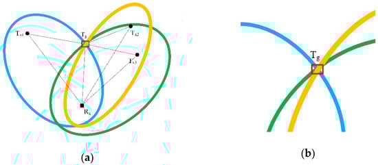
Figure 2.
(a) Schematic diagram of Bistatic Range (BR) positioning error, (b) Particular section.
In the multistatic radar system, in order to achieve multistatic network information selection and optimize multistatic positioning, bistatic T/R pairs with good positioning performance can be selected according to certain criteria. For this purpose, this paper proposes two algorithms for the selection of external illuminators.
3. Selection Methods of Bistatic T/R Pairs
3.1. Covariance Matrix Fusion Method
The principle of this method is to select bistatic T/R pairs from a multistatic radar system based on resolution unit, to minimize the overlap area of the elliptical rings, equivalent to minimizing the positioning error. The presentation diagram of this method is shown in Figure 3.
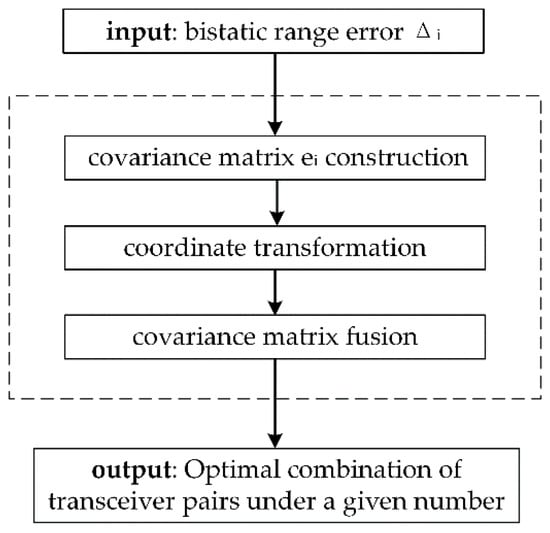
Figure 3.
Presentation diagram of Covariance Matrix Fusion Method.
First, the range information is used to construct the covariance matrix , which describes the positioning error of the bistatic T/R pair. The matrix obtained by the weighted fusion of is the inscribed ellipsoid covariance matrix of the overlap area. The volume of the overlap area is proportional to the determinant of [36]. So, the criterion for selecting bistatic T/R pairs is equivalent to optimizing with the smallest determinant after the matrix fusion. Next, for easy understanding, we directly construct the inverse matrix of , and express it as follows.
where represents the bistatic range measurement error, which is mainly related to the multistatic geometric configuration, the signal bandwidth and the sampling frequency. As shown in (13), , where is the modulus of bistatic range vector . and , with being the speed of light (about ), being the signal bandwidth, being the sampling frequency of the satellite signal and being the weighting factor.
Equation (12) is obtained in the target local coordinate with the bisector as the axis. Different bistatic geometries correspond to different target local coordinates, hence, while we conduct the following covariance matrix fusion, the covariance matrix must be transformed into the same coordinate, defined as the local coordinate. The classic 7-parameter coordinate rotation method is used (see (A1) (A2) in the Appendix A) to realize the coordinate transformation, and the covariance matrix in the local coordinate can be written as:
with being the rotation matrix from the bistatic coordinate into the local coordinate. Finally, the optimization problem can be obtained as follows:
where, is the weighting factor.
By solving the above question, the optimal combination of bistatic T/R pairs can be obtained. It can be seen that the method can select the optimal combination of a given number of T/R pairs. Although the result may not be the most effective, for the multistatic radar system, we can use the method to do a reasonable rough selection of multiple bistatic pairs to reduce the amount of system calculations.
3.2. Convex Hull Optimization Method
Convex hull problem is a classic problem in the computer geometry. In a real vector space , for a given set , the intersection of all convex sets containing is called the convex hull of [37]. The convex hull concept provides another algorithm to solve the problem in the paper.
The main idea to formulate the T/R pair selection criteria as a convex hull problem bases on resolution capability. First, we define a vector for the bistatic T/R pair to represent its capability of the range resolution. The vector is along the direction of and its modulus value is , where being the bistatic range variance as discussed in the last subsection. represent the endpoints of all vectors , and let the point set , then, the smallest convex polygon (polyhedron) that encloses all vertices in is called the convex hull of . On 2-D plane, minimizing the positioning error is equivalent to maximizing the area of the polygon expanded by the vector endpoints. Correspondingly, in 3-D space, it is equivalent to maximizing the volume of the polyhedron with the vector endpoints expanded.
Figure 4 is demonstrated in 2-D for visualization, and the target localization problem of this paper is solved in 3-D. The red dot in the figure indicates starting point of , and the black dots and the gray dots indicate endpoints, which are also the data set of the convex hull method. The dotted arrow is to more intuitively reflect the modulus of , that is, to reflect positioning error of each bistatic T/R pair. It can be seen that the smaller the positioning error, the more likely it is to be selected as vertex of the convex hull. These vertices (the black dots in Figure 4) form the selected bistatic T/R pair combination.
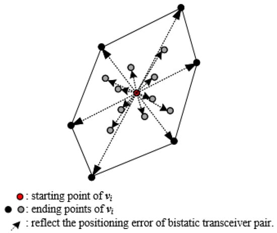
Figure 4.
Schematic diagram of 2-D convex hull.
In 3-D space, the specific coordinate position of is calculated as follows:
where is the angle between and the Z axis, is the angle between the projection of on the XOY plane and the positive half axis of X axis, and is the angle between the projection of on the XOY plane and the positive half axis of Y axis.
The presentation diagram of the proposed method is shown in Figure 5, and the specific description is as follows.
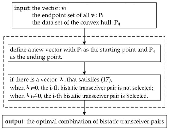
Figure 5.
Presentation diagram of Convex Hull Optimization Method.
First, we define a new vector that takes as the starting points and as the endpoints. Next, if there is a vector that satisfies (17), then, when , it indicates that the bistatic vector is not on the convex hull, so its corresponding T/R pair is not selected. When , the bistatic T/R pair is selected. In this way, we get the optimal combination of bistatic T/R pairs.
The computational complexity of the proposed method is , and is the number of bistatic T/R pairs. Compared with other 3-D convex hull algorithms, the computational complexity of proposed method is equivalent to that of the incremental method , and is less than the extreme point method and the extreme edge method [38]. The proposed method is also suitable for the calculation of convex hull of arbitrary dimensions.
4. Simulation and Experimental Results
An experiment is conducted to evaluate the performance of Covariance Matrix Fusion Method (CMF method) and Convex Hull Optimization Method (CHO method). They are verified through maritime target positioning experiment using the GNSS-based passive multistatic radar.
4.1. Experimental Scene and Conditions
The experimental scenario and a GNSS passive receiver are shown in Figure 6. The multistatic radar system is formed with multiple GNSS transmitters of opportunity, including GPS L1, GLONASS G1, and Galileo E5a and E5b. The passive receiver is installed to receive GNSS signals in the east of Portsmouth harbor in the UK, and it has two receiving channels. One receives the direct wave signal, and the other receives the target echo signal. The bandwidth of this receiver can cover the four GNSS bands which are recorded simultaneously at a sampling rate of 20 MHz. When the large target moves relatively close to the receiver, it can provide a sufficiently high SNR.
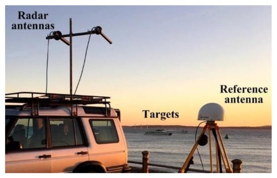
Figure 6.
The experimental scene.
We located a commercial ferry (the “St. Cecilia”) whose length is 77m and beam is 17.2m, as shown in Figure 7. During the experiment, the ferry entered the port at a low speed, so we can know the time of departure and arrival of the ferry in advance. In addition, Automatic Identification System (AIS) installed on the ship can record the ferry’s driving in real time, which provides us with ground reference data for multistatic positioning.

Figure 7.
The photo of the “St. Cecilia”.
There are 12 visible satellites during the data acquisition period. All through the experimental recording, these satellites continuously illuminate the targets. The satellite geometry topology is shown in Figure 8.
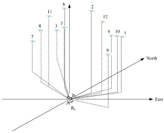
Figure 8.
Geometry topology of 12 visible satellites.
And information on these satellites can be found in Table 1.

Table 1.
Satellite parameters.
4.2. Experimental Results of CMF Method
The selection of bistatic T/R pairs is equivalent to select visible satellites in the GNSS-based passive multistatic radar. Therefore, CMF method is used to select the optimal combinations of 4, 5, …, 11 satellites from 12 visible satellites. Using AIS data as a reference, we calculate Root Mean Square (RMS) of the optimal combinations. At the same time, the theoretical error is calculated as the reference for the upper limit of positioning performance. The specific calculation process will not be repeated in this paper, which has been demonstrated in literature [29]. And the error curves of CMF method are shown in Figure 9.
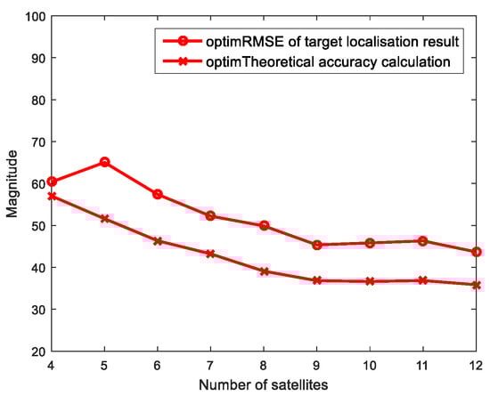
Figure 9.
The positioning error of the Covariance Matrix Fusion (CMF) method.
As shown in Figure 9, the positioning error is still in the trend: the measured RMS and the theoretical result both decrease as the number of satellites increases. It is not difficult to see that there are still some small fluctuations in the measured RMS curve in the figure. The reason for this phenomenon is that when observing complex targets such as aircrafts and ferries, these targets can be regarded as a collection of many independent scatterers. When scatterers are unstable, a small change on the viewing angle will cause the echoes synthesized by each scatterer to produce larger fluctuations, thereby affecting the positioning effect of these complex targets.
In addition, in order to evaluate the performance of CMF method more intuitively, we also compared the measured RMS and the theoretical results before and after selecting satellites (Figure 10 and Figure 11), respectively. From Figure 10 and Figure 11, the measured RMS curve and the theoretical result curve after selecting satellites by CMF method are obviously lower than those before selection, that is, the positioning error is significantly reduced. It shows that positioning accuracy has been improved after selecting satellites, and shows the correctness of the proposed method.
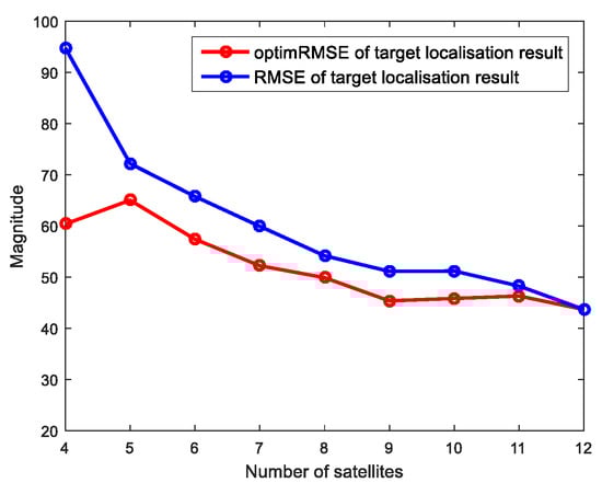
Figure 10.
Comparison of the measured Root Mean Square (RMS) before and after selection.
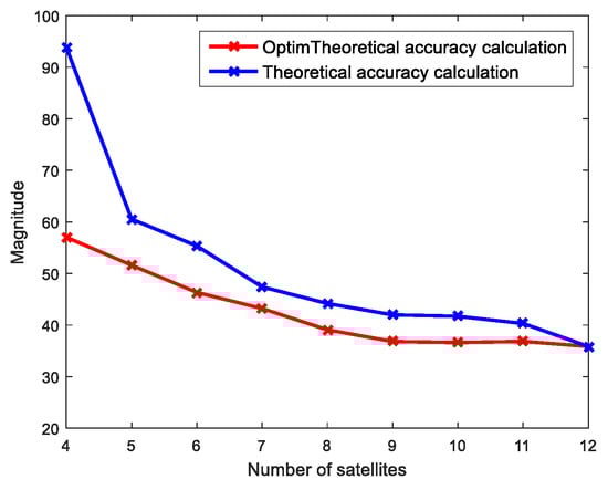
Figure 11.
Comparison of theoretical accuracy before and after selecting.
4.3. Experimental Results of CHO Method
We use the CHO method to select an optimal combination of 6 satellites from 12 visible satellites. The positioning results are shown in Figure 12c and Table 2.
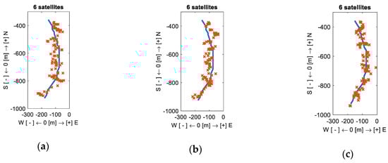
Figure 12.
The positioning results before and after selecting: (a) The positioning result without selecting, (b) The positioning result of the CMF method, (c) The positioning result of the Convex Hull Optimization (CHO) method.
Table 2.
Positioning error analysis for target by the CHO method (6 satellites).
In Figure 12, it is ‘North Up’, so East is to the right and the blue solid line is the AIS track used as a reference, and the red “×” indicates all target positions obtained using a certain number of satellites, and the marking step is 1s.
In contrast, the red “×” marks are more condensed around the solid blue line in Figure 12c, and it shows that the positioning result obtained by CHO method is more accurate. In more detail, we can see Table 2. Under the same number of satellites (6 satellites), the measured RMS and the theoretical result of CHO method is reduced by 14.8632m and 13.9223m, respectively, and optimizations by CMF method are reduced by 8.3538m and 9.0115m, respectively. Moreover, before selecting satellites, the difference between the measured RMS and the theoretical result of 6 satellites is 10.4446m. After the CHO method selection, the difference between them is 9.4637m. It means the positioning accuracy has been improved. Finally, comparing Table 2 and Table 3, we can see that the error of CHO method is even smaller than that of 7, 8, 9, and 10 satellites without selecting. Through comparison of various aspects, it is concluded that CHO method has good satellite selection capabilities.
Table 3.
Positioning error analysis for target without selecting.
4.4. The Case of a Larger Number of Satellites
To further specify the selection performance of proposed methods in the case of more transmitters, further simulation have been conducted. The simulation parameters are set most practically, using the ephemeris of all the four GNSS constellations (BDS, GPS, GLONASS, and Galileo). In the simulation, the positions of 55 satellites used are shown in Figure 13.
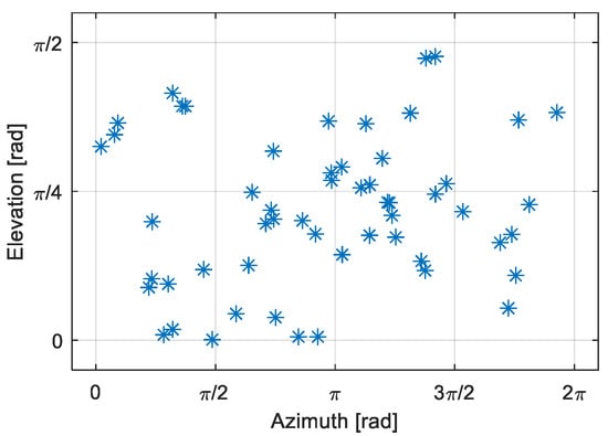
Figure 13.
Satellite location diagram.
The bistatic range variance of each T/R pair is expressed as , where Q is the coefficient. The selection results of the CHO method are shown in Table 4.
Table 4.
CHO method selection results.
From Table 4, 31 satellites are selected from 55 satellites using CHO method, which greatly reduces the amount of calculation for multistatic satellite signal processing. At the same time, the positioning error of this method is equivalent to that of 55 satellites, which is significantly smaller than the error of randomly selecting 31 satellites, and it further illustrates the effectiveness of this method for selecting satellites. However, it also shows that changing the range measurement error does not change the satellite selection results. This is because when the level of the range measurement error is equivalent, once the multistatic geometry and the system parameters are certain, the number of satellites filtered out are determined.
When the total number of satellites is very large, the number of satellites selected by CHO method is still a lot. At this time, we can use the CMF method to select again, and can also select the specified number of satellites according to the actual computing power. When Q = 15, the selection result of the combination of CHO and CMF is shown in Figure 14.
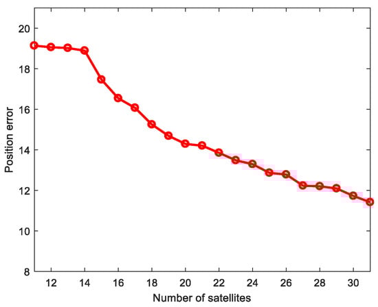
Figure 14.
CMF method selection result.
4.5. Discussion of the Algorithm Limitations
In the last decade, an explosive growth has been witnessed of the GNSS, Starlink, and other satellites. This brings opportunities for the passive radars, but an effective selection of satellites also becomes a fundamental issue to be considered. The passive radar could not, after all, achieve a real-time processing of all satellite sources. As shown in Figure 15, we have summarized the signal processing of the GNSS-based multistatic radar. The most computational section lies in the two-dimensional coherent integration of the range compression and Doppler processing, because of the high sampling frequency in the fast-time domain. Hence, the computational burden is approximately proportional to the number of the selected satellites.
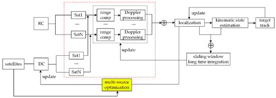
Figure 15.
Schematic diagram of Global Navigation Satellite System (GNSS)-based multistatic radar signal processing.
Based on the above, two algorithms are proposed for the transmitter-selection problem of the passive radar when they are more than enough. The effectiveness of both algorithms has been verified by the simulation and experimental results. However, the two methods have their own advantages and limitations. First, the two methods are under a same premise that the approximate target position is known, which is generally a target-tracking mode, however, when the target position deviation is too large, the performance of proposed methods can be affected. Further analysis will be conducted in the follow-up work.
Second, for the CMF method, the positioning accuracy after selection is also limited by the choice of the covariance matrix construction method and the matrix fusion algorithm. While for the CHO method, once the multistatic geometry is certain, the number of satellites filtered out are determined, which lacks the flexibility. Nevertheless, a combination of the two methods can address this problem, that the CMF could be applied after the CHO selection.
5. Conclusions
The multistatic radar system is the developmental trend of the radar research. From a different perspective, the systems composed of more than two receivers or more than two transmitters have been studied and defined as the netted radar, MIMO radar, or multistatic radar. With the increasing scale of the system, the consequent problem is the huge computational load of the signal processing. Therefore, cognitive mechanism needs to be considered to select the transmitter and receiver pair and to limit the scale of the origin datasets, but still retain the performance of the multistatic systems.
Therefore, based on the study of the multistatic positioning, this paper proposes two multi-source selection algorithms to optimize the multistatic target localization precision. The first method, the CMF method, is a classic multistatic fusion method based on the ranging covariance matrix. The second, the CHO method, is based on the ranging vector, which is more commonly used in navigation and positioning optimization. We learn from it to evaluate the target localization capability of the multistatic radar system.
The theoretical derivations have shown the mechanism of the two methods. To validate the theoretical model, experiments were conducted using GNSS satellites as the multiple illuminators using one receiver. More than ten satellites were seen in the experimental results, and both algorithms have good selecting capabilities and can retain the accuracy of multistatic target localization, utilizing a fewer number of satellites. When the same number of satellites are selected, the CHO method is more effective. However, in cases of larger number of transmitters or receivers, the two methods can be combined to achieve a more effective selection, for which the simulation has been conducted with 55 GNSS satellites. From the simulation results, to obtain the same level of localization precision, at least one third of the computational load can be reduced.
The proposed methods can be extended to any multistatic radar systems, which can contribute to the practical real-time multistatic radar applications.
Author Contributions
All authors have made significant contributions to this manuscript. Conceptualization, S.Z.; methodology, H.M.; validation, Y.S., resources, M.A.; writing—original draft preparation, Y.S.; writing—review and editing, H.M.; project administration, X.W.; funding acquisition, H.L. All authors have read and agreed to the published version of the manuscript.
Funding
This research was funded by the National ScienceFund for Distinguished Young Scholars (No. 61525105), the Fundfor Foreign Scholars in University Research and Teaching Programs (the 111 Project No. B18039), the program for Cheung Kong Scholars, the Postdoctoral Innovation Talent Support Program, the National Natural Science Foundation of China(No. 61901344), the National Defense Foundation of China, the foundation of Science and Technology on Electronic Information Control Laboratory, Chinese Postdoctoral Science Funding and the National Natural Science Foundation of Shaanxi Province (No. 2019JQ-289). (Corresponding author: Hui Ma.)
Institutional Review Board Statement
Not applicable.
Informed Consent Statement
Not applicable.
Data Availability Statement
Data sharing is not applicable to this article, because the raw/processed data required to reproduce these findings also forms part of ongoing study.
Acknowledgments
Special thanks to Jun Wang for his guidance on this paper.
Conflicts of Interest
The authors declare no conflict of interest.
Appendix A
According to the rotation order of the ZXZ axis, we use Euler angles to construct the rotation matrix :
where, are the rotation matrices, and the three rotation angles are shown in Figure A1.

Figure A1.
Schematic diagram of coordinate system rotation.
References
- Liu, J.Y. Research on Anti-Spoofing Jamming Method of Multi-Static Radar System; Xidian University: Xi’an, China, 2018. [Google Scholar]
- Ye, F. Research on Anti-Radiation Missile Imaging and Recognition Technology Based on Distributed Passive Radar; Xidian University: Xi’an, China, 2009. [Google Scholar]
- Griffiths, H. Multistatic, MIMO and networked radar: The future of radar sensors. In Proceedings of the 7th European Radar Conference, Paris, France, 30 September–1 October 2010; pp. 81–84. [Google Scholar]
- Lan, J.J.; Chen, B.; Xu, T.X. Development status of netted radar and its jamming technology. Fly. Missile 2009, 12, 39–41. [Google Scholar]
- Zheng, G.Q.; Zheng, Y. Radar netting technology & its development. In Proceedings of the 2011 IEEE CIE International Conference on Radar, Chengdu, China, 24–27 October 2011; pp. 933–937. [Google Scholar]
- Liu, J.Y.; Chen, X.H.; Liu, Q.; Sun, J.Z. Development Status and Key Technology Analysis of Foreign Bistatic (Multistatic) Radar. Fly. Missile 2013, 6, 54–59. [Google Scholar]
- Greco, M.S.; Stinco, P.; Gini, F.; Farina, A. Cramer-Rao Bounds and Selection of Bistatic Channels for Multistatic Radar Systems. IEEE Trans. Aerosp. Electron. Syst. 2011, 47, 2934–2948. [Google Scholar] [CrossRef]
- Zhao, Y.B.; Liu, H.W. Review of MIMO radar technology. Data Acquis. Process. 2018, 33, 389–399. [Google Scholar]
- Fishler, E.; Haimovich, A.; Blum, R.S.; Cimini, L.J.; Chizhik, D.; Valenzuela, R.A. Spatial Diversity in Radars—Models and Detection Performance. IEEE Trans. Signal Process. 2006, 54, 823–838. [Google Scholar] [CrossRef]
- Donnet, B.J.; Longstaff, I.D. MIMO Radar, Techniques and Opportunities. In Proceedings of the 2006 European Radar Conference, Manchester, UK, 13–15 September 2006; pp. 112–115. [Google Scholar]
- Wang, H.H. RFS Multi-Target Tracking Algorithm and Its Application in Passive Radar; Xidian University: Xi’an, China, 2017. [Google Scholar]
- Fan, Y. Multistatic Radar Target Information Fusion Method and Its Application; Wuhan University: Wuhan, China, 2018. [Google Scholar]
- Wang, B.D. The Role of Bistatic/Multistatic Radar in Modern High-Tech Warfare; Chinese Institute of Electronics: Beijing, China, 2000; pp. 84–91. [Google Scholar]
- Li, X.; Zhu, Y.; Li, B. Optimal anti-jamming strategy in sensor networks. In Proceedings of the IEEE International Conference on Communications (ICC), Ottawa, ON, Canada, 10–15 June 2012; pp. 178–182. [Google Scholar]
- Chen, Y.G.; Li, X.H.; Shen, Y. Multistatic Radar Combat Capability Analysis and Evaluation; National Defense Industry Press: Beijing, China, 2006. [Google Scholar]
- Li, X.Y. Development and key technologies of bistatic/multistatic radar. Radar Countermeas. 2013, 33, 4–8. [Google Scholar]
- Wang, T.C.; Yang, J.W.; Zhao, H.S.; Ma, D.J. “Silent Sentinel” system and its core technology. Mil. Commun. Technol. 2009, 30, 89–93. [Google Scholar]
- Huang, X.; Tang, H.; Niu, C.; Zhang, J. Analysis of passive radar anti-stealth technology and its development trend. Fly. Missile 2012, 3, 31–35. [Google Scholar]
- Zhou, B.X. A brief introduction to the history and development of Russian radar. Electron. Eng. Inf. 2010, 4, 37–48. [Google Scholar]
- Zhao, Q.L. Multistatic Radar Target Positioning and Site Error Correction; Xidian University: Xi’an, China, 2015. [Google Scholar]
- Zhang, Z.; Zhou, F.; Zhang, L.L. An active/passive radar cooperative detection and tracking algorithm. J. Air Force Eng. Univ. (Science Edition) 2013, 14, 51–55. [Google Scholar]
- Zhou, F.; Zhang, L.L.; Wang, J.J.; Zhang, Z. Research on a mode and algorithm of active/passive radar cooperative detection and tracking. Electron. Opt. Control 2014, 2, 12–16. [Google Scholar]
- Chen, Y.Y.; Xie, J. Maneuvering target tracking algorithm based on passive time difference positioning system. Electron. Sci. Technol. 2012, 25, 61–65. [Google Scholar]
- Chaudhuri, S.P. A General Approach to the Development of Passive/Active Sensor Data Fusion. In Proceedings of the 1985 American Control Conference, Boston, MA, USA, 19–21 June 1985; pp. 823–828. [Google Scholar]
- Wu, X.Z. Research on the Joint Processing Method of Cognitive Radar Transmitting and Receiving; Xidian University: Xi’an, China, 2017. [Google Scholar]
- Ma, H.; Antoniou, M.; Pastina, D.; Santi, F.; Pieralice, F.; Bucciarelli, M.; Cherniakov, M. Maritime Moving Target Indication Using Passive GNSS-Based Bistatic Radar. IEEE Trans. Aerosp. Electron. Syst. 2018, 54, 115–130. [Google Scholar] [CrossRef]
- Pastina, D.; Santi, F.; Pieralice, F.; Bucciarelli, M.; Ma, H.; Tzagkas, D.; Antoniou, M.; Cherniakov, M. Maritime Moving Target Long Time Integration for GNSS-Based Passive Bistatic Radar. IEEE Trans. Aerosp. Electron. Syst. 2018, 54, 3060–3083. [Google Scholar] [CrossRef]
- Pieralice, F.; Pastina, D.; Santi, F.; Bucciarelli, M. Multi-transmitter ship target detection technique with GNSS-based passive radar. In Proceedings of the International Conference on Radar Systems (Radar 2017), Belfast, UK, 23–26 October 2017; pp. 1–6. [Google Scholar] [CrossRef]
- Ma, H.; Antoniou, M.; Stove, A.G.; Winkel, J.; Cherniakov, M. Maritime Moving Target Localization Using Passive GNSS-Based Multistatic Radar. IEEE Trans. Geosci. Remote Sens. 2018, 56, 4808–4819. [Google Scholar] [CrossRef]
- Santi, F.; Pieralice, F.; Pastina, D. Joint Detection and Localization of Vessels at Sea With a GNSS-Based Multistatic Radar. IEEE Trans. Geosci. Remote Sens. 2019, 57, 5894–5913. [Google Scholar] [CrossRef]
- Ma, H.; Antoniou, M.; Stove, A.G.; Cherniakov, M. Target Kinematic State Estimation with Passive Multistatic Radar. IEEE Trans. Aerosp. Electron. Syst. 2018, 56. [Google Scholar] [CrossRef]
- Antoniou, M.; Cherniakov, M. Experimental demonstration of passive GNSS-based SAR imaging modes. In Proceedings of the IET International Radar Conference, Xi’an, China, 14–16 April 2013; pp. 1–5. [Google Scholar] [CrossRef]
- Santi, F.; Pastina, D.; Antoniou, M.; Cherniakov, M. GNSS-based multistatic passive radar imaging of ship targets. In Proceedings of the 2020 IEEE International Radar Conference (RADAR), Washington, DC, USA, 28–30 April 2020; pp. 601–606. [Google Scholar] [CrossRef]
- Zhao, Y.S.; Zhao, Y.J.; Zhao, C. Multi-static and multi-external emitter passive location algorithm based on bistatic range. Acta Electron. 2018, 46, 2840–2847. [Google Scholar]
- Malanowski, M.; Kulpa, K. Two Methods for Target Localization in Multistatic Passive Radar. IEEE Trans. Aerosp. Electron. Syst. 2012, 48, 572–580. [Google Scholar] [CrossRef]
- Yu, H.T.; Zhang, Y.S.; Qi, L.F. Calculation and Analysis of the Positioning Accuracy of a Multistatic Radar System. J. Air Force Eng. Univ. (Natural Science Edition) 2005, 6, 8–11. [Google Scholar]
- Hao, X.J. Research on Acceleration and Improvement of Convex Hull Algorithm; Hebei University of Technology: Tianjin, China, 2003. [Google Scholar]
- De Berg, M.; van Kreveld, M.; Overmars, M.; Schwarzkopf, O. Computational Geometry: Algorithms and Applications; Springer: Berlin/Heidelberg, Germany, 2005. [Google Scholar]
Publisher’s Note: MDPI stays neutral with regard to jurisdictional claims in published maps and institutional affiliations. |
© 2021 by the authors. Licensee MDPI, Basel, Switzerland. This article is an open access article distributed under the terms and conditions of the Creative Commons Attribution (CC BY) license (http://creativecommons.org/licenses/by/4.0/).