Canopy Top, Height and Photosynthetic Pigment Estimation Using Parrot Sequoia Multispectral Imagery and the Unmanned Aerial Vehicle (UAV)

Abstract

Remote sensing is one of the modern methods that have significantly developed over the last two decades and, nowadays, it provides a new means for forest monitoring. High spatial and temporal resolutions are demanded for the accurate and timely monitoring of forests. In this study, multi-spectral Unmanned Aerial Vehicle (UAV) images were used to estimate canopy parameters (definition of crown extent, top, and height, as well as photosynthetic pigment contents). The UAV images in Green, Red, Red-Edge, and Near infrared (NIR) bands were acquired by Parrot Sequoia camera over selected sites in two small catchments (Czech Republic) covered dominantly by Norway spruce monocultures. Individual tree extents, together with tree tops and heights, were derived from the Canopy Height Model (CHM). In addition, the following were tested: (i) to what extent can the linear relationship be established between selected vegetation indexes (Normalized Difference Vegetation Index (NDVI) and NDVI_{red edge}) derived for individual trees and the corresponding ground truth (e.g., biochemically assessed needle photosynthetic pigment contents) and (ii) whether needle age selection as a ground truth and crown light conditions affect the validity of linear models. The results of the conducted statistical analysis show that the two vegetation indexes (NDVI and NDVI_{red edge}) tested here have the potential to assess photosynthetic pigments in Norway spruce forests at a semi-quantitative level; however, the needle-age selection as a ground truth was revealed to be a very important factor. The only usable results were obtained for linear models when using the second year needle pigment contents as a ground truth. On the other hand, the illumination conditions of the crown proved to have very little effect on the model’s validity. No study was found to directly compare these results conducted on coniferous forest stands. This shows that there is a further need for studies dealing with a quantitative estimation of the biochemical variables of nature coniferous forests when employing spectral data that were acquired by the UAV platform at a very high spatial resolution.

1. Introduction

Forests play a significant role in the Earth’s ecosystems and they contribute greatly to reducing adverse climate change impacts. They provide a natural environment for many species of animals and plants, represent a significant carbon sink, and support an effective hydrological cycle. In addition, forests serve as an important source of timber and other non-wood materials [1,2]. At the beginning of the 1980s forest health and the sustainability of their ecosystems became a highly discussed topic for politicians, the public, and scientists due to the aforementioned functions of forests and the increasing level of damage they suffer [3].

In Europe, temperate forests are mainly affected by climate change and air pollution [4,5]. During the 20th century, the region on the Czech, Polish, and German borders was influenced by extensive coal mining, which was linked to large emissions of SO₂ and NOx from power plants [6,7]. In order to monitor the process of ecosystem recovery after the reduction in pollution that started in the 1980s and accelerated in the 1990s, the Geochemical Monitoring network of small catchments (GEOMON) was initiated across the Czech Republic. Since 1993, when the GEOMON network began, the data that were collected from observations of these catchments have been used for many studies [7,8] mainly corresponding to catchment biogeochemistry (e.g., [6,9,10,11,12,13]). The recent study that was published by Švik et al. [7] supplied the aforementioned research that was based on field observations using remote sensing methods that have been also employed in this study.

Remote sensing techniques have been frequently used to study forest areas for multiple purposes over the last decade. They have been proven to be less costly and time-consuming alternatives to ground level research [14]. Satellite and aerial imagery have offered an opportunity to investigate forests at the regional scale, for example, to estimate forest biomass, monitor forest cover changes, or classify types of biome [15,16,17,18]. The use of airborne multispectral and hyperspectral sensors has led to closer forest observation, such as the classification of tree species, monitoring forest health, or estimating chlorophyll content [19,20,21,22,23,24]. The newly developed Unmanned Aerial Vehicles (UAV) complement the established remote sensing (RS) methods. UAVs have increased the number of benefits, such as acquiring extreme high-spatial resolution data, flexibility in usage and over time, and the capacity to carry various sensors, such as a multispectral camera, to observe vegetation health [25,26].

Most of the studies use a combination of UAV complemented by a multispectral sensor to analyse agriculture crops for precision farming (e.g., tomato, vineyard, or wheat production), where they usually employ Vegetation Indices (VIs), such as the Normalized Difference Vegetation Index (NDVI), the Green Normalized Difference Vegetation Index (GNDVI), or the Soil Adjusted Vegetation Index (SAVI), to monitor crop health [27,28,29,30,31,32]. Authors monitoring vineyards described the use of multispectral and thermal sensors in combination to obtain additional information about crop water status [33,34,35].

When assessing the foliage traits of forest trees, it is necessary to take the tree size, branch geometry, and tree density, respectively, foliage clumping into account [36]. Dealing with evergreens, particularly conifers, a higher level of complexity emerges as different needle age generations contribute to the final signal received by the sensor. These might be the main reasons why, despite the high potential of UAVs, not many studies have dedicated an analysis of multispectral data for assessing forests. Recently, UAV-based multispectral sensing has been used for high-throughput monitoring of the photosynthetic activity in a white spruce (Picea glauca) seedling plantation [37]. A few more studies on forest health assessment using the UAVs and multispectral cameras have been published so far. Dash et al. [38] demonstrated the usefulness of such approaches for monitoring physiological stress in mature plantation trees, even during the early stages of tree stress when using a non-parametric approach for the qualitative classification. Chianucci et al. [39] used the true colour images, together with a fixed-wing UAV, to quantify the canopy cover and leaf area index of beech forest stands. Dash et al. [40] tested the sensitivity of the multispectral image data time-series that were acquired by the UAV platform and satellite imagery to detect herbicide-induced stress in a controlled experiment conducted on a mature Pinus radiata plantation. Other successful qualitative forest classifications have been demonstrated while using UAVs together with multispectral [41,42] and hyperspectral cameras [43,44]. A pioneer approach for estimating tree-level attributes and multispectral indices using UAV in a pine clonal orchard was recently published by Gallardo-Salazar and Pompa-García [45]. All of these studies listed above deal with qualitative forest classifications, so, a need for quantitative approaches, focusing on forest biochemical variable estimations employing UAV-based multispectral sensing, is clearly demanded.

For such quantitative spectral-based approaches, which employ very high-spatial resolution data, an accurate definition of the extent of individual trees is a crucial task. The delineation of a tree crown boundary has been studied before and several approaches to detect individual trees have been published. Lim et al. [46] applied a segmentation method to the RGB orthoimage and the Canopy Height Model (CHM) that was obtained by UAV. A similar approach using multispectral data instead was described in Díaz-Varela et al. [47]. A popular technique is hydrological terrain analysis–watershed algorithm, where the inverse CHM is delineated by the watershed algorithm, where catchment basins represent individual trees and holes substitute tree peaks [15,48,49,50]. Among the recent methods are the LiDAR point cloud segmentation [51,52], which achieves highly accurate results [48,53,54,55,56,57] and also approaches that employ deep learning techniques to detect individual trees [58,59].

This study tested, if a UAV that is equipped with a multispectral camera can be employed for photosynthetic pigment estimation in coniferous trees. As already described, when assessing coniferous forests, such factors as tree size and density affect the validity of estimations of structural forest parameters [36]. Moreover, as different needle age generations contribute to the final image pixel reflectance, it is still not clear what ground truth should be optimally used (e.g., [60]). To fill these gaps, two small catchments (part of the GEOMON network in Czech Republic) inhabited by mainly mature Norway spruce monocultures were selected as test sites based on their relatively close spatial proximity, alongside differences in parent material, which significantly influenced nutrient availability for forest ecosystems. The images from a Multi-spectral Unmanned Aerial Vehicle (UAV) were acquired over these two sites, and the following topics were researched:

• An accurate definition of the individual tree extents (crown delineation) and derivation of other parameters, such as tree top and height using the UAV-based multispectral data.
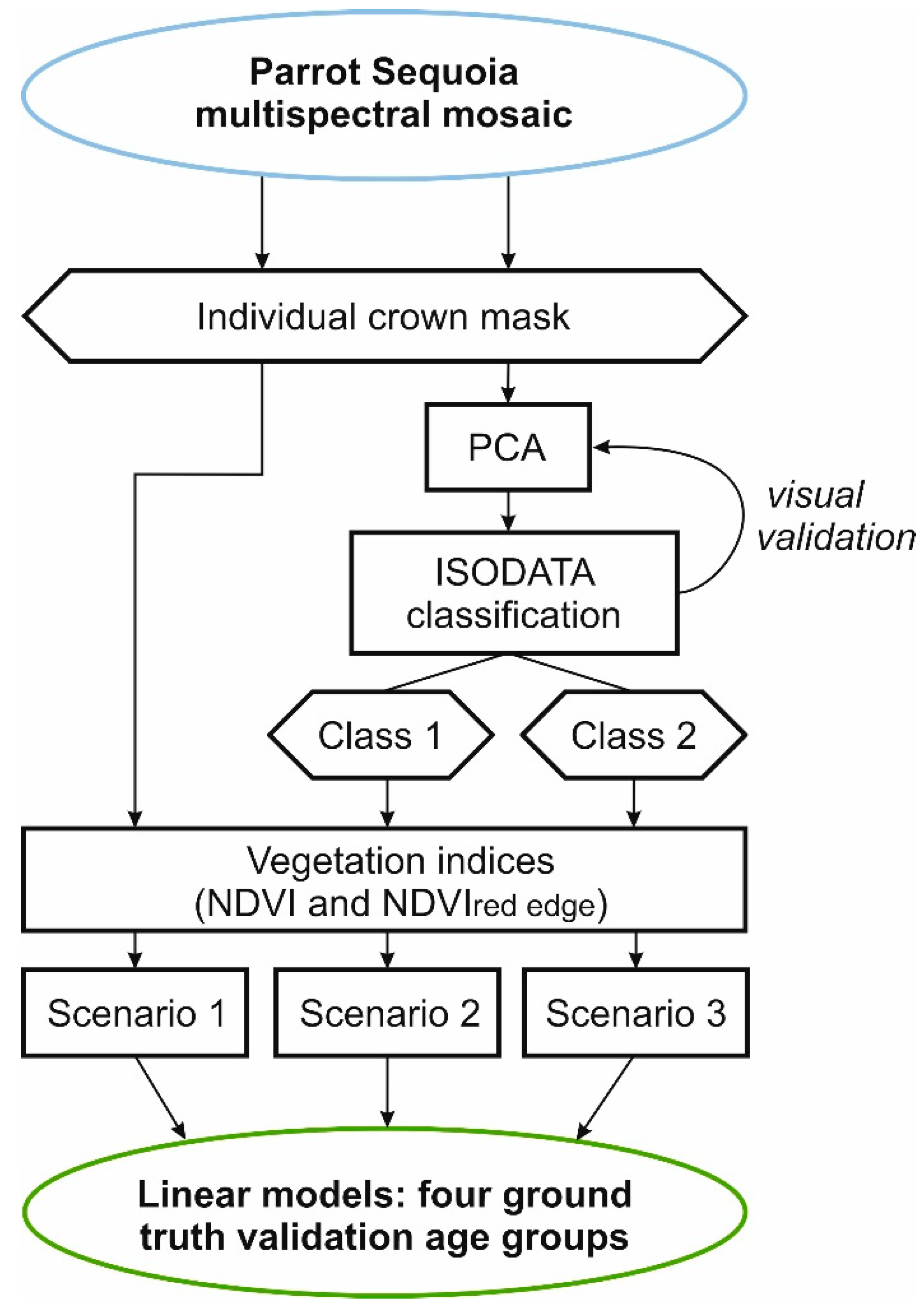
• Testing if a linear relationship can be established between selected vegetation indices (NDVI and NDVI_{red edge}) that are derived for individual trees and the corresponding ground truth (e.g., biochemically assessed needle photosynthetic pigment contents).
• Testing whether the needle age selection, as ground truth affects the validity of the linear models.
• Testing if the tree crown light conditions affect the validity of the linear models.

2. Materials and Methods

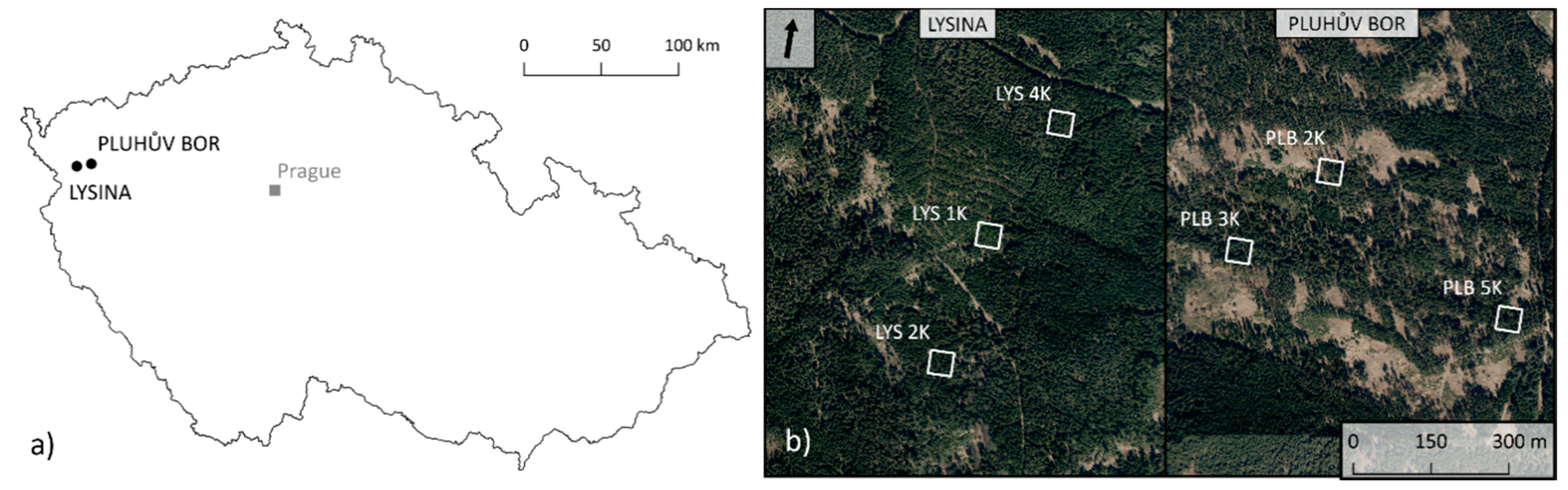
2.1. Test Sites

Two test sites representing rural mountainous landscapes in the western part of Bohemia were selected—Lysina (LYS) and Pluhův Bor (PLB) (Figure 1). These two catchments have been part of the European network—GEOMON established in 1993 to assess changes in precipitation and stream chemistry after reducing pollution in Eastern Europe. The selected catchments were heavily affected by acid pollution during the 20th century. Nowadays, both sites are part of the Slavkov Forest Protected Landscape Area. The vegetation cover mostly consists of managed Norway spruce monocultures [10], which are situated around 800 ma.s.l. The main difference between these two sites is the lithology and soil type as well as the forest age.

Table 1. Characteristics of selected catchments: Lysina and Pluhův Bor [10].

Site	Bedrock	Soils	Elevation (m a. s. l.)	Forest Age (Year Range)	Spruce Forest (ha)	Broadleaf Forest (ha)	Non- Forested Area (ha)
LYS	Granite	Cambisols, Podzols	880	12–53	27	0.0	0.4
PLB	Serpentinite	Magnesic Cambisols, Stagnic–Magnesic Cambisols, Magnesic Gleysols	755	41–129	18	0.0	4.0

and

Table 2. Tree ages at the two catchments selected in this study.

Test Site	Average Age	Min Age	Max Age
LYS 1K	14	12	17
LYS 2K	16	15	18
LYS 4K	47	44	53
PLB 2K	120	109	129
PLB 3K	72	70	74
PLB 5K	47	41	50

provides detailed catchment characteristics.

2.2. In-situ Ground Truth

In this study, three tree stands were selected in the LYS catchment (LYS 1K, LYS 2K, and LYS 4K) and three stands in the PLB catchment (PLB 2K, PLB 3K, and PLB 5K), these stands were the object of previous long-term research, thus the soil conditions were known as well as tree height information, which was measured in-situ and modelled using the LiDAR data [62].

To follow up with the previous research activities, the same trees described in Lhotáková et al. [60] were selected at each stand (three trees per stand, in total 18 trees). The branch samples were collected by a climber from the sunlit crown part one day before the UAV-based data were acquired (August 2018). The needle age was identified and three different age classes were sampled: first, second, and a mixed sample of fourth year and older needles (hereinafter referred to as 4th year for simplicity) [60]. The needles were cooled and immediately transported to the laboratory where they were kept at a stable temperature at −20 °C until further processing. Photosynthetic pigments—chlorophyll a, b and total carotenoids—were extracted in dimethylformamide following the procedures described in detail by Porra et al. [63] and then spectrophotometrically determined [64].

2.3. UAV Data Acquisition

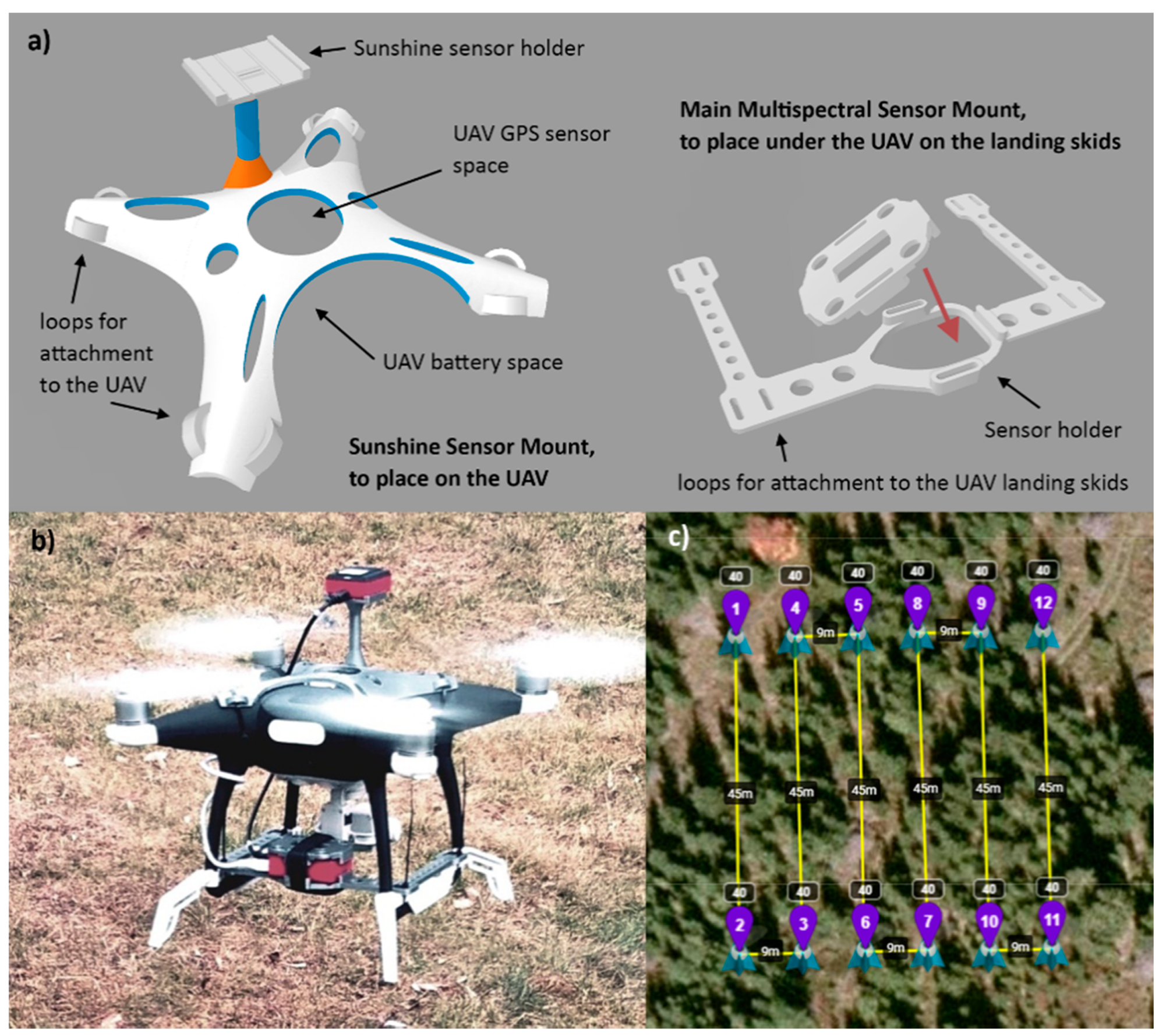
2.3.1. Equipment

In this experiment, an unmanned aerial vehicle DJI Phantom 4 (SZ DJI Technology Co., Ltd. [65]) was employed (Figure 2b). It is a widely used quadcopter weighing 1380 g with an RGB camera in 4K (4096 × 2160 px) [66]. The UAV was complemented by a multispectral camera Parrot Sequoia scanning system (senseFly Inc. [67]). The camera was specially designed to support vegetation studies; therefore, besides Red and Green bands, there is a band placed in the Red edge region as well as one band in the Near infrared (NIR) (

Table 3. Overview of a Parrot Sequoia spectral band setting.

Band Name	Spectral Range (nm)	Central Wavelength (nm)
Green	530–570	550
Red	640–680	660
Red edge (RE)	730–740	735
Near infrared (NIR)	770–810	790

).

The Parrot Sequoia consists of two parts—the main camera and a sunshine sensor calibrating the measured spectral radiation by the main sensor. These two parts of the multispectral camera were attached to the drone by mounts that were designed by the CGS team (Figure 2a). The 3D models of mounts were created in CAD software. It was important to make a free space for the GPS sensor to ensure good signal reception. The holder for the sunshine sensor had to be placed in a manner, so as not to have any contact with the propellers (Figure 2a). The mounts were printed using the Prusa i3 3D printer (Prusa Research a.s. [68]).

2.3.2. Data Acquisition

The RGB and Parrot Sequoia multispectral data were obtained for both test sites. The flights were made on 6 and 7 August 2018, between 11 am and 3 pm to ensure the multispectral camera captured the required maximum reflected sunlight and eliminate shadows. Prior to data acquisition, a flight path was planned in the flylitchi.com web tool (Figure 2c), which was connected to the litchi android application (VC Technology Ltd. [69]) controlling the UAV. Areas of 40 × 40 m² were defined to cover the tree groups and their surroundings. All of the flight paths covering the area of interest were planned in a north-south direction and in a way so the parallel scanning lines would reach 70% of the side overlap in order to ensure errorless image mosaicking when creating photogrammetric products. The flight height was set up according to the highest terrain point (40–70 m above ground level) and it was 25–30 m above the treetops. The UAV speed was set at 3.6 km/h to ensure well-focused images were recorded. Sequences of images were recorded every two seconds (s) with 95% overlap in the direction of the flight. The resulting spatial resolution of RGB imagery varied between 1.1–1.9 cm/px and 3.76–6.59 cm/px for multispectral imagery, respectively, according to flight height.

Regarding multispectral data calibration, images of the calibrated reflectance panel were acquired before and after each flight. The same routine was used for each flight—the calibration target (Aironov) was placed on the ground and the UAV was held above the panel always keeping the same position—the Sun was behind the UAV, so no reflection and shadow were affecting the panel, as this was recommended by the manufacturer. The same rules were applied to the other cameras (e.g., [70]).

GPS data from DJI Phantom 4 and Parrot Sequoia camera were used to reference the resulting orthomosaics into the coordinate system (WGS 84/UTM 33N). The imaging data (RGB and multispectral bands) were processed in Agisoft Metashape software (Agisoft LLC [71]), which allowed for orthomosaics (RGB and multispectral) and digital surface models (DSMs) to be created using the structure from motion method [72]. The multispectral data calibration was automatically made by the Agisoft Metashape software, which detected the images of the calibrated panel by the QR code in it as described in [73].

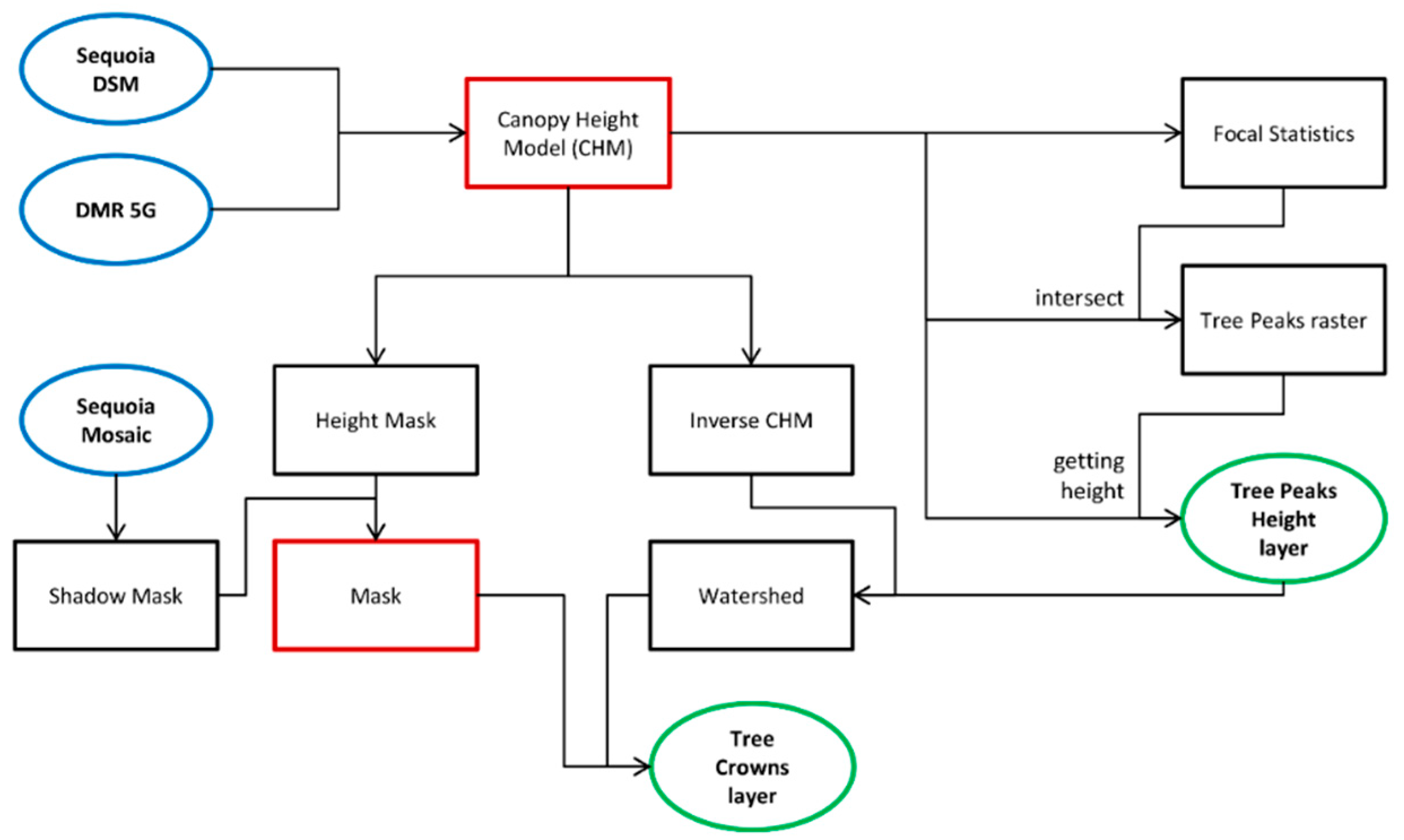
2.4. Tree Height, Crown and Top Detection

Tree height detection was based on the Canopy Height Model (CHM) described as the difference between treetop elevation and the underlying ground-level elevation [74]. In this study, the 5th Digital Elevation Model (DEM) generation (DMR 5G; [61,75]) was used as a source of ground-level information, while treetop information was obtained from the digital surface model (DSM) that was obtained from the Parrot Sequoia camera multispectral images (Seq DSM):

CHM = Seq DSM − DMR 5G

(1)

First, the DMR 5G data (original spatial resolution 0.5 m) were resampled to a Seq DSM spatial resolution of 16–25 cm, and Seq DSM was calibrated by DMR 5G elevation to obtain proper results. The calibration was performed at each site by extracting the average heights from the Seq DSM of a clearing or forest path, then it was possible to compare this height value with the average site altitude derived from the DMR 5G. The elevation of the Seq DSM was then corrected by this difference.

The following procedure was employed to derive tree tops. Focal statistics was employed to the CHM raster to get rid of noisy pixels and a new dataset was created (CHMfoc). The best results were achieved when using the maximum value and a 5 × 5-pixel window, according to the empirical tests carried out [76]. A window with a smaller size caused frequent double peak detection. On the other hand, a bigger window did not identify a sufficient number of tree peaks. The tree tops were detected by identifying the local maxima in the CHMfoc raster. The representative pixels for the highest CHMfoc values were then identified in the original CHM raster, as it was important to keep the original pixel positions and values and the treetop point layer was derived [49]. Figure 3 shows the tree height detection workflow.

In order to delineate the tree crowns, the workflow described by Jaakkola et al. [50] was followed, which used watershed analysis to identify tree crown borders using the CHM derived from UAV-based laser scanning. First, inverse CHM (iCHM) was created, where trees were visualized as depressions and treetops represented the lowest points in the digital elevation model:

iCHM = CHM * (−1)

(2)

The iCHM, together with the tree peak layer representing pour points, were used to compute watershed regions. The watershed analysis showed good results, even in the case of splitting two or multiple nearby standing trees (Figure 4a). Tree borders in places with no connection to another tree crown were defined using a height mask (Figure 4b), more specifically excluding such areas where the CHM altitude was at least 3 m lower than the actual lowest detected tree. This allowed for the space under the tree crowns to be removed. Consequently, to only visualise sunlit crown parts convenient for the following multispectral analyses, the shadow mask was derived by thresholding the Red band of the multispectral mosaic (Seq Mosaic) and selecting values lower than 0.04 [77]. In the next step, the height mask was merged with the shadow mask (Figure 4c). The final tree crown boundaries were obtained by applying the merged mask to the watershed layer (Figure 4d), as a result the individual tree crowns were extracted.

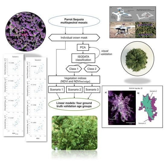
2.5. Multispectral Data Processing

The Parrot Sequoia camera captures four-band images (Green, Red, Red edge, and Near infrared), which were specifically designed for vegetation analysis (Table 3). These bands allow computing, for instance, the Normalized Difference Vegetation Index (NDVI) [78], which is a universal vegetation index, but also, more importantly, they allow the modification of NDVI when using the Red edge band instead of the Red band. Red Edge Normalized Difference Vegetation Index (NDVI_{red edge}) has been used to assess vegetation stress [79], as the stress directly affects the wavelength position of the red-edge inflexion point on the electromagnetic spectrum [80,81]. The NDVI_{red edge} index is defined as:

$$\frac{\mathrm{NIR}-\mathrm{RE}}{\mathrm{NIR}+\mathrm{RE}}$$

(3)

where NIR is the Near infrared band and RE is the Red edge band of the Parrot Sequoia camera.

This study tested whether a linear relationship can be established between these two popular vegetation indices (VIs) and the ground truth (e.g., biochemically assessed needle photosynthetic pigment contents). The individual tree crown pixels were delineated in the multispectral images while using the iCHM-based approach (described in detail in Section 2.4). Moreover, the UAV-based imaging data provided at exceptionally high spatial resolution provided an opportunity to test whether the crown geometry and light conditions affect the crown VI values and the estimation of the photosynthetic pigments (the validity of the linear models), respectively. Therefore, the intention was to delineate crown parts that receive higher and lower illumination. First, Principal Component Analysis (PCA) [82] was employed to reduce the four-band dimensionality into three bands (PC1–PC3) and display them as an RGB composition. PC1–PC3 were then visually assessed to check whether it is possible to classify the detected tree crowns according to different illumination conditions. For simplicity, these three Principal Components (PC1–PC3), which covered the majority of the information variability, were selected as the input for the subsequent unsupervised classification employing the Iterative Self-Organizing Data Analysis Technique (ISODATA; [83]). A preliminary ISODATA classification was initially set to yield a maximum of four classes; these classes were then recoded into two classes based on the visual inspection when using the RGB ortho-photomosaics, which were provided at the highest spatial resolution for all image products.

It was then possible to define three scenarios for further analysis of the multispectral data (Figure 5):

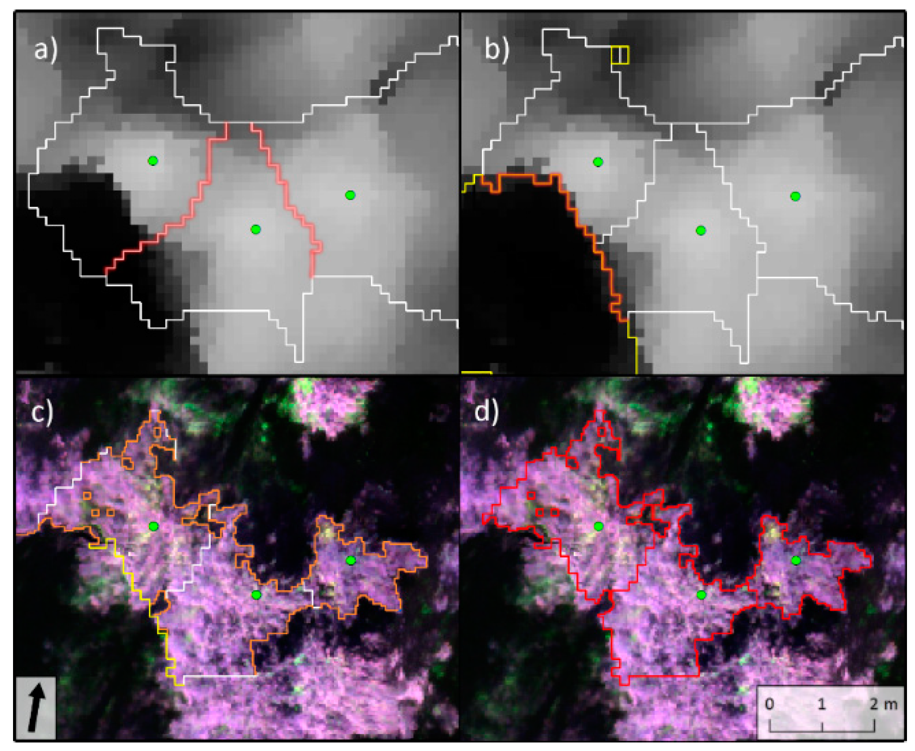
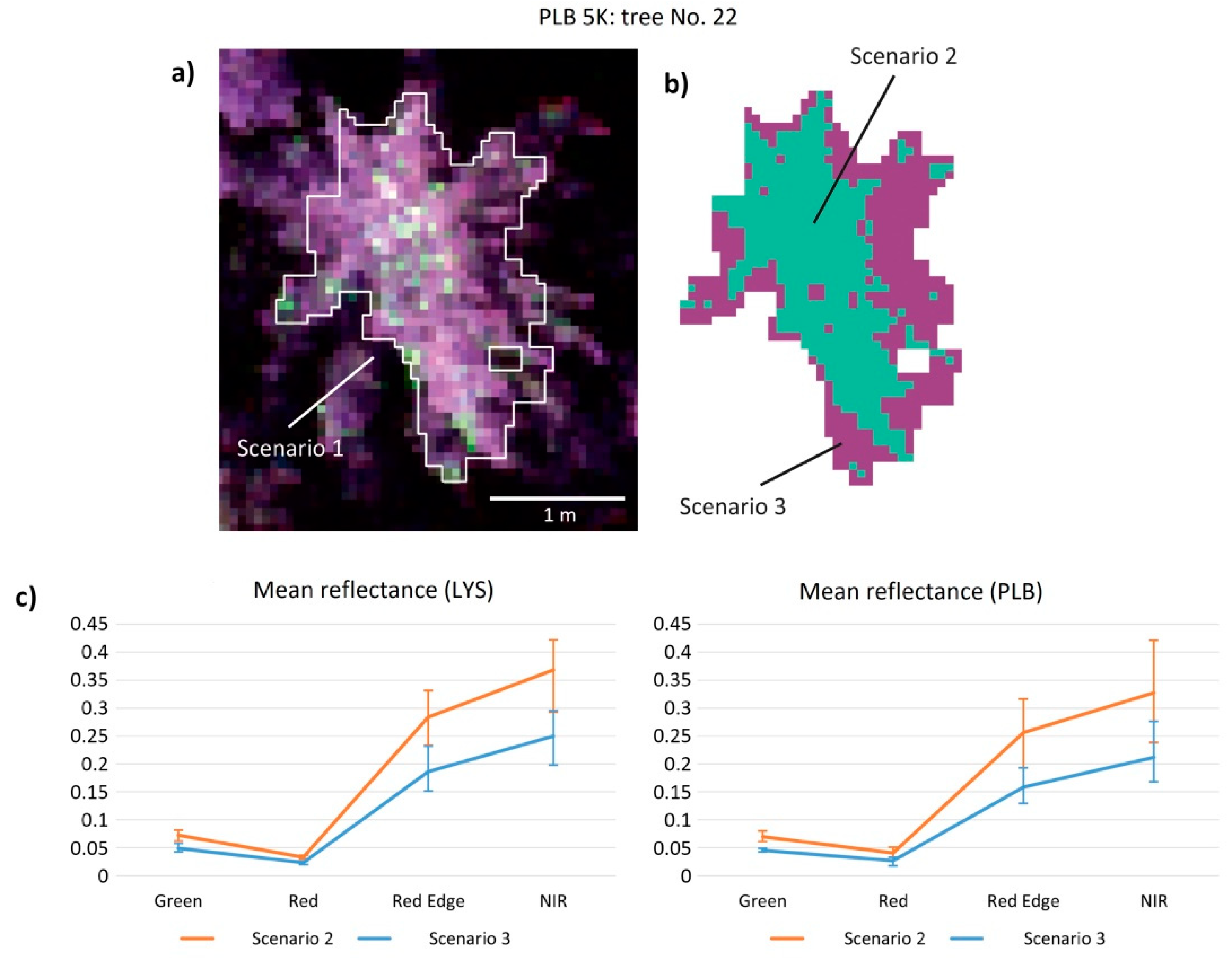
• Scenario 1: all of the pixels representing the whole tree crown have been averaged and used for further statistical analysis.
• Scenario 2: pixels representing the higher-illumination top part of the crown have been averaged and used for further statistical analysis.
• Scenario 3: pixels that represent the lower-illumination part of the crown have been averaged and used for further statistical analysis.

For each scenario, a linear model between the derived VI values and corresponding ground truth (needle photosynthetic pigment contents defined in the laboratory) was individually constructed. Different needle age generations contribute to the final image pixel reflectance; however, it is still not clear what the optimal ground truth age proportion is, as already mentioned. The recommendation given by [60] was followed to include not only current (first year) but also older needles as a ground truth and four ground truth validation age groups were thus created:

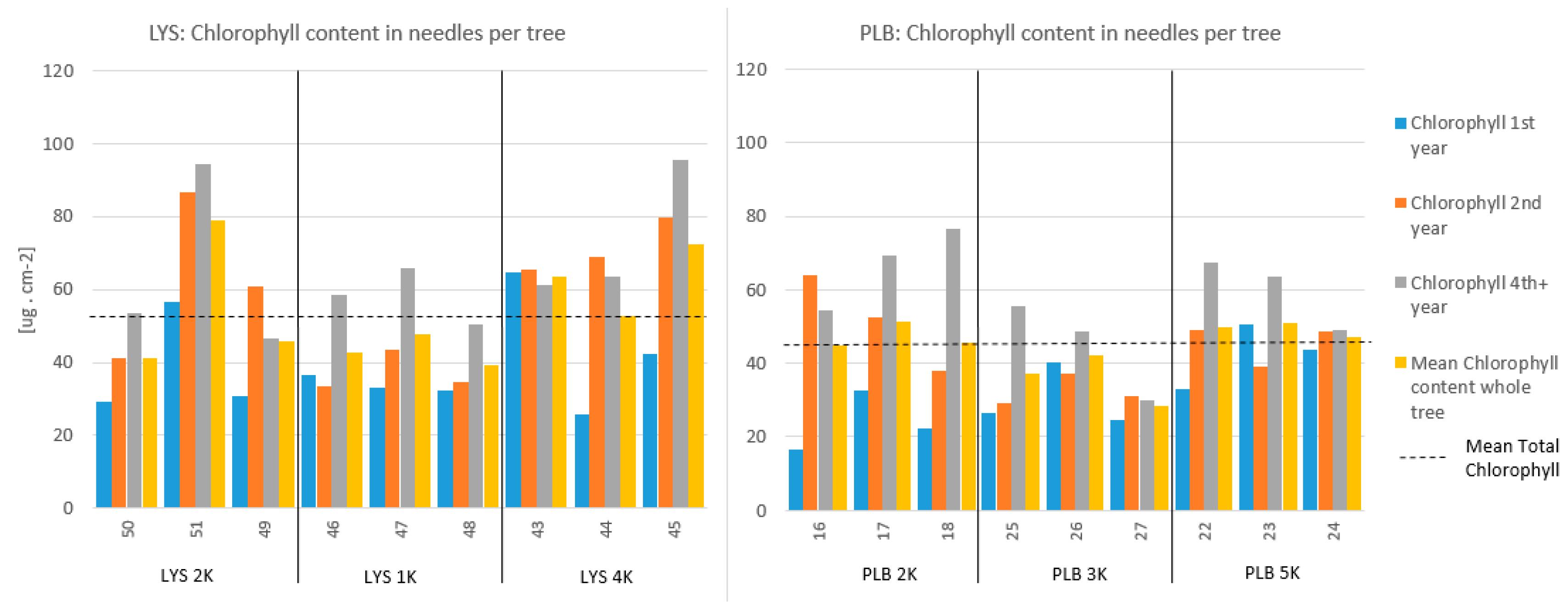
• all needles included
• first year needles included
• second year needles included
• mixed sample of fourth year and older needles (hereinafter referred to as fourth year for simplicity)

To evaluate the linear models, the coefficient of determination (R²) was used:

$${\mathrm{R}}^2=1-\frac{S{S}_{res}}{S{S}_{tot}}$$

(4)

where SS_res represents the residual sum of squares and SS_tot represents total sum of squares [84].

3. Results

3.1. Photosynthetic Pigments

Laboratory analyses of needles that were collected as a ground truth showed typical chlorophyll and carotenoid values (

Table 4. Mean contents of photosynthetic pigments based on in-situ needle samples for both catchments.

	Catchment	All Needles	1st Year Needles	2nd Year Needles	4+ Years Needles
Total Chlorophyll (µg·cm−2)	Lysina (LYS)	52.580	35.756	56.055	65.399
	Pluhův Bor (PLB)	44.425	31.148	43.895	57.172
Chlorophyll a (µg·cm−2)	Lysina (LYS)	37.939	26.124	40.679	46.637
	Pluhův Bor (PLB)	32.071	22.810	31.989	40.672
Chlorophyll b (µg·cm−2)	Lysina (LYS)	14.641	9.631	15.373	18.761
	Pluhův Bor (PLB)	12.354	8.343	11.904	16.500
Carotenoids (µg·cm−2)	Lysina (LYS)	6.724	4.400	7.018	8.602
	Pluhův Bor (PLB)	5.596	3.451	5.284	7.591

) for non-stressed mature Norway spruce trees in a similar region and at a similar altitude [60,85]. This was despite the fact that forest in the PLB catchment showed evidence of suppressed growth due to the nutritional stress that is caused by the extreme chemistry of the underlying bedrock [86]. This further indicated that photosynthetic pigment content alone provided a somewhat limited indication of stressed trees. At both of the study sites, almost all trees exhibited the usual accumulation of chlorophyll and carotenoids in older needles in comparison with the first year needles (Table 4) [22,85,87,88,89,90].

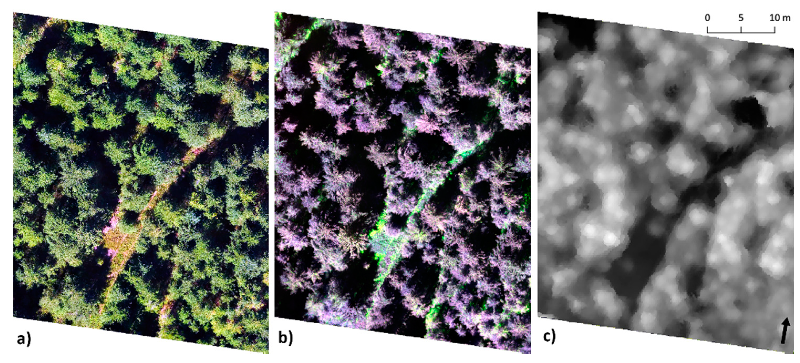
3.2. UAV Photogrammetric Products

The UAV data were acquired over three stands in the Lysina catchment (LYS 1K, LYS 2K, and LYS 4K) and three stands in the Pluhův Bor catchment (PLB 2K, PLB 3K, and PLB 5K). At each stand, the DSM, RGB, and multispectral orthomosaics were created (Figure 6).

Table 5. The resulting spatial resolution and photogrammetric model errors of multispectral and RGB data.

	Parrot Sequoia-Multispectral Camera				DJI Camera-RGB
Test Site	DSM (cm/px) (Seq DSM)	Orthomosaic (cm/px) (Seq Mosaic)	Vertical Error (m)	Total Error (m)	Orthomosaic (cm/px)	Total Error (m)
LYS 1K	23.95	5.99	0.78	1.02	2.26	0.77
LYS 2K	16.41	4.09	0.55	0.67	1.12	1.14
LYS 4K	19.64	4.91	0.65	0.94	2.17	0.79
PLB 2K	23.30	5.82	0.51	0.82	2.05	0.71
PLB 3K	24.47	6.11	0.53	0.74	2.36	1.27
PLB 5K	23.00	5.74	0.61	0.72	1.87	0.83

shows the resulting spatial resolution and photogrammetric model errors. The total errors of the photogrammetric products oscillated around 1 m. The calculated vertical error of DSMs varied between 0.51 and 0.78 m, and the obtained accuracy was comparable with the results that were published for an DJI Phantom 4 UAV [91]. The RGB data from DJI Phantom 4 were then mainly used for a visual control, while the calibrated multispectral data were used for further statistical assessment.

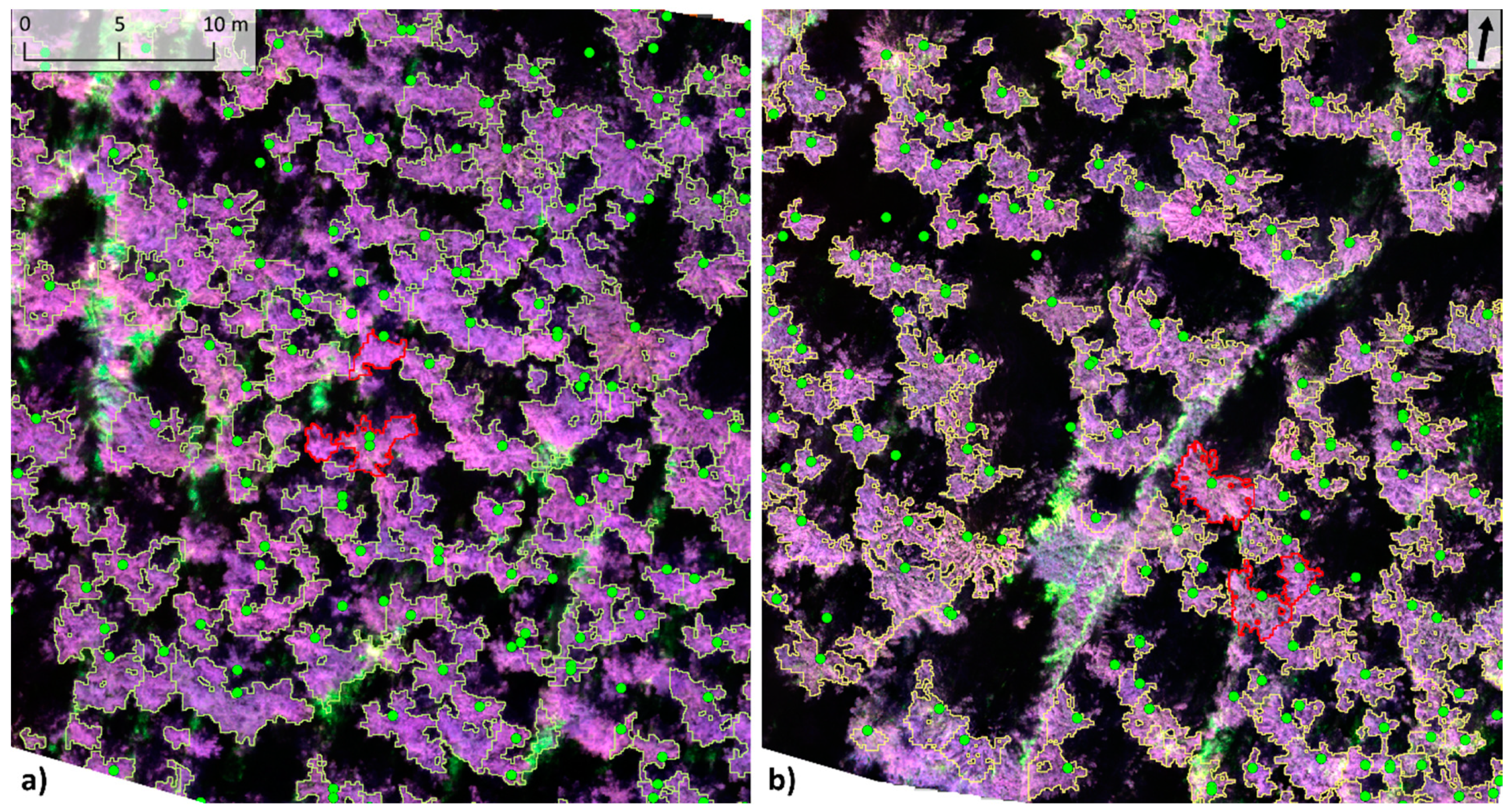
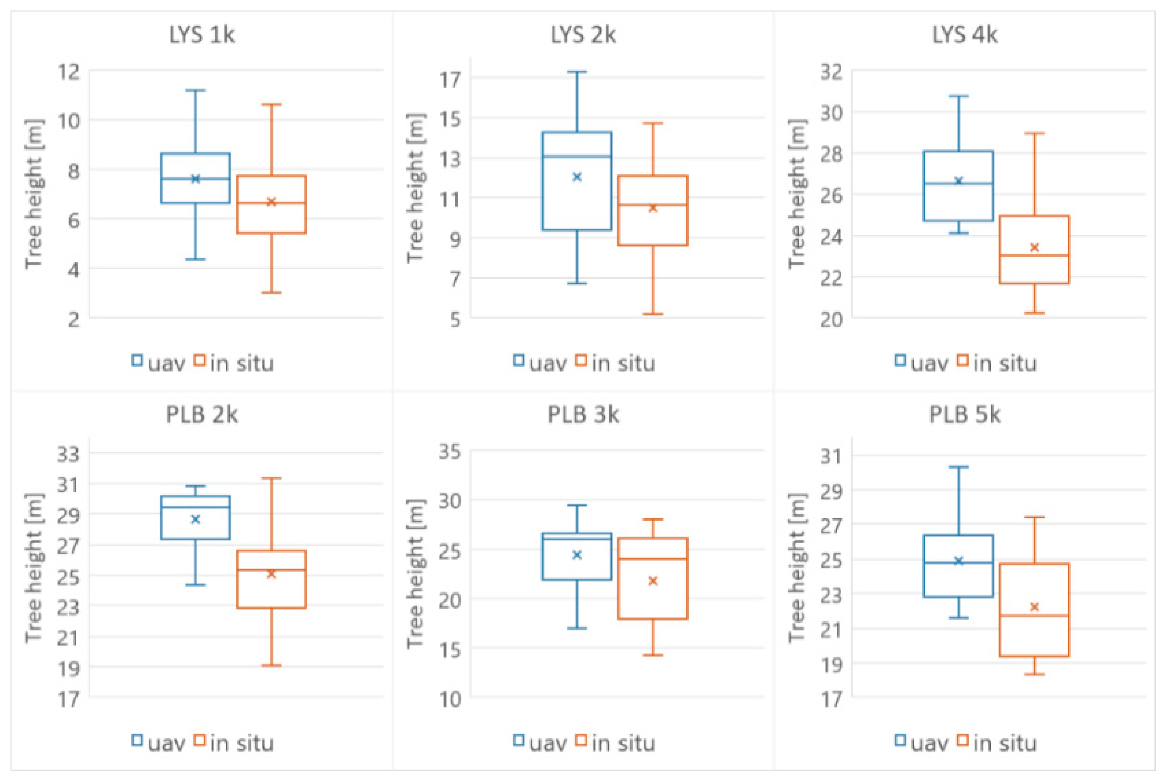
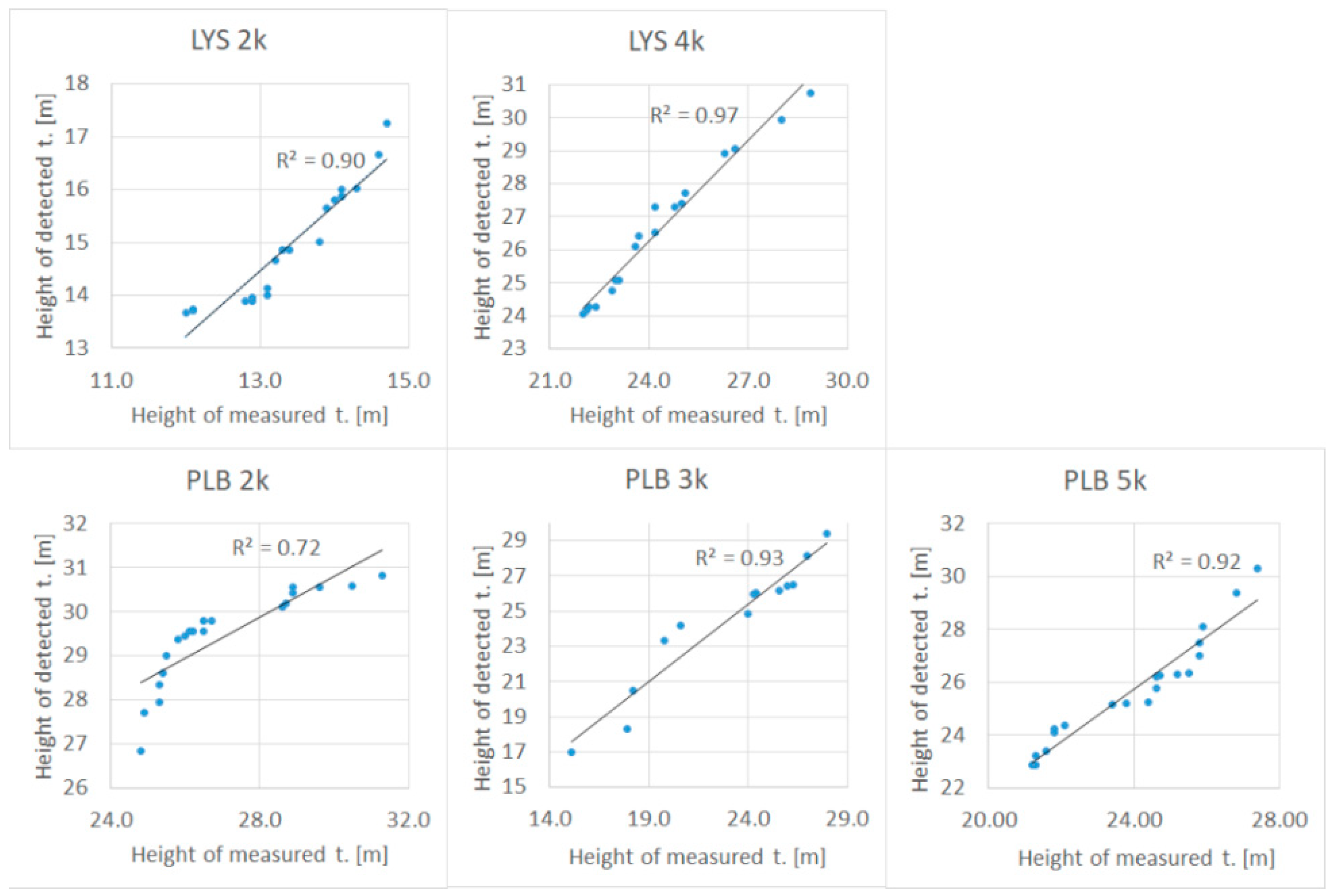
3.3. UAV Tree Height, Crown and Top Detection

The tree characteristics—height, crown, and top—derived from the CHM raster (Figure 7) were compared with the in-situ measurements that were collected in 2015 [62].

Table 6. Comparison between the number of detected tree peaks and crowns (Canopy Height Model (CHM)-estimated) and in-situ measured data.

Test Site	No. of Trees Measured In-Situ (Above Set Height Mask)	No. of Detected Tree Peaks Based on UAV Data	Success Rate of Detected Tree Tops (%) (Compared to the Trees Measured In-Situ)	No. of Detected Tree Crowns Based on UAV Data	Success Rate of Detected Tree Crowns (%) (Compared to the Trees Measured In-Situ)
LYS 1K	177	45	25.42	61	34.46
LYS 2K	67	49	73.13	57	85.07
LYS 4K	25	18	72.00	19	76.00
PLB 2K	34	25	73.53	31	91.18
PLB 3K	15	13	86.66	17	86.67
PLB 5K	32	26	81.25	34	93.75

summarizes the evaluation statistics. One stand—LYS 1K—showed very high error; for the other stands, the success rate for the tree top identification varied between 72 and 87%. When checking the in-situ data for LYS 1K, it was found that this stand is represented by significantly younger trees with the highest trees measured around 12 m. At this particular stand the trees were very dense and rather short, therefore tree detection could be problematic. As this stand also obtained very high errors in all other statistics, it was defined as an outlier and excluded from further statistics. In the case of tree crown estimation, the comparable success rate achieved varied between 76–94% (Table 6). In two cases, PLB 3K and PLB 5K, the tree crown detection results showed a higher number of estimated numbers than those that were measured in the field. This could be possibly caused by false crown splitting when using the tree shadow mask in the detection algorithm.

The box plots showing the distributions of tree height values for all stands—CHM-derived and in-situ—are displayed in Figure 8. Furthermore, either all trees were validated (LYS 4K—18 trees and PLB 3K—13 trees) or a comparable yet representative number—in this case, the 20 tallest trees—were selected to validate the bigger stands (LYS 2K, PLB 5K, and PLB 2K). The averaged CHM-estimated tree height values were compared with the in-situ data. It can be concluded that the tree height values that were derived for these trees from CHM were always higher than the in-situ measurements, the differences ranged between 1.54–2.36 m (

Table 7. Comparison of average tree heights of the 20 tallest trees for each stand: CHM-estimated tree heights and the situ measured data.

Test Site	Average Tree Top Height (m)-In-Situ Data	Average Tree Top Height (m) Based on the CHM Data	Difference of Average Tree Heights (m)
LYS 2K	13.33	14.87	1.54
LYS 4K	24.34	26.62	2.28
PLB 2K	27.08	29.44	2.36
PLB 3K	22.86	24.63	1.77
PLB 5K	23.95	25.70	1.75

). These differences are most probably a combination of the vertical error of the Seq DSM (0.51–0.78 m; Table 5) and tree growth between the years 2015 and 2018. Based on a relationship between the tree diameter at breast height (DBH) and height [62], the 2015–2018 average height increment was estimated to be 1.1 ± 0.5 m at Lysina and 0.4 ± 0.2 m at Pluhův Bor. However, the correlation between the estimated heights of the 20 tallest trees using CHM and in-situ measured data was high (Figure 9), as the coefficients of determination (R²) obtained were higher than 0.90 in four out of five cases.

3.4. Tree Crown Illumination Classes

The first three Principal Components (PC1–PC3) covered more than 99% of the crown spectral variability (

Table 8. Principal Component Analysis (PCA) statistics obtained for tree crowns analysed at the two sites: Lysina (LYS) and Pluhův Bor (PLB) catchments.

LYS
PC Component	Eigenvalue	Variance	Cumulative Variance
1	0.01602	98.6427	98.6427
2	0.00015	0.9405	99.5832
3	0.00006	0.3733	99.9566
4	0.00001	0.0434	100
PLB
PC Component	Eigenvalue	Variance	Cumulative variance
1	0.021	99.0774	99.0774
2	0.00014	0.6383	99.7157
3	0.00005	0.2335	99.9493
4	0.00001	0.0507	100

), and they were used as the input for the subsequent unsupervised ISODATA classification. The classification results were visually validated using the ortho-photomosaics (RGB and multispectral), and the best results were achieved using the following set up (maximum iterations 30, maximum class standard deviation 1, maximum class distance 5, and change threshold 5%). It was concluded that the final classification enabled a differentiation between the higher (Scenario 2) and lower-illuminated (Scenario 3) parts of a crown. Figure 10a,b give an example of tree No. 22 (PLB 5K stand), showing the distribution of the two final illumination classes within the tree crown and Figure 10c shows the mean reflectance derived for the two illumination scenarios per watershed. Clearly, Scenario 2 contains pixels that receive higher-illumination (overall higher reflectance, significantly higher mean, minimum, and maximum values in the Red Edge-NIR region) and Scenario 3 includes pixels that receive the lower illumination (overall lower reflectance, significantly lower mean, minimum, and maximum values in the Red Edge-NIR region). Zhang et al. [92] described the same trend at the leaf level.

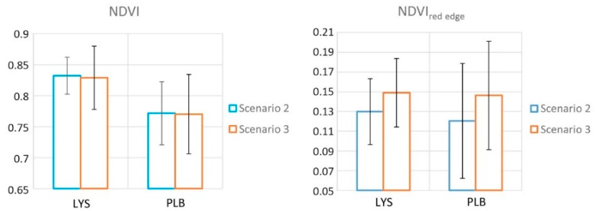
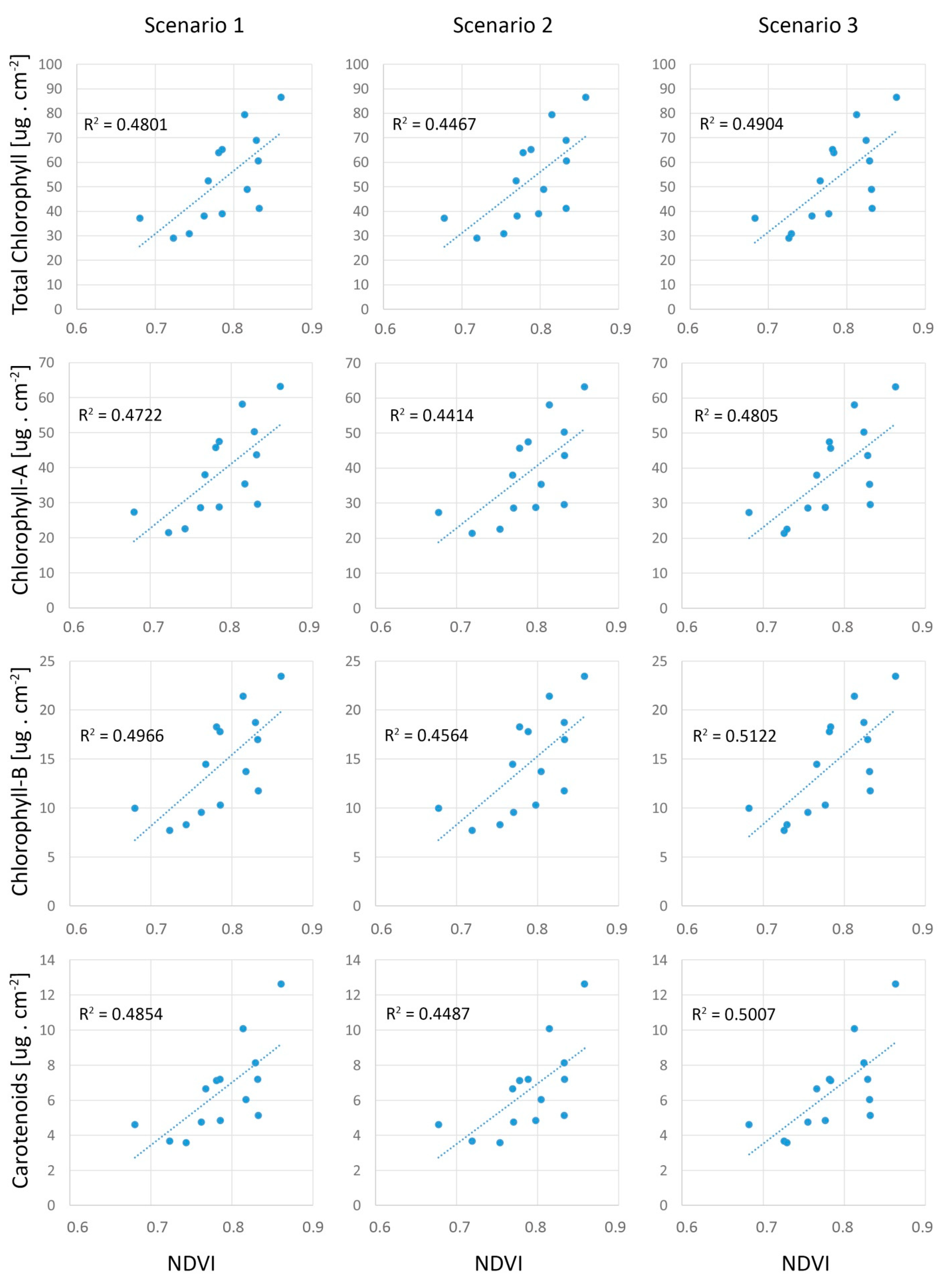
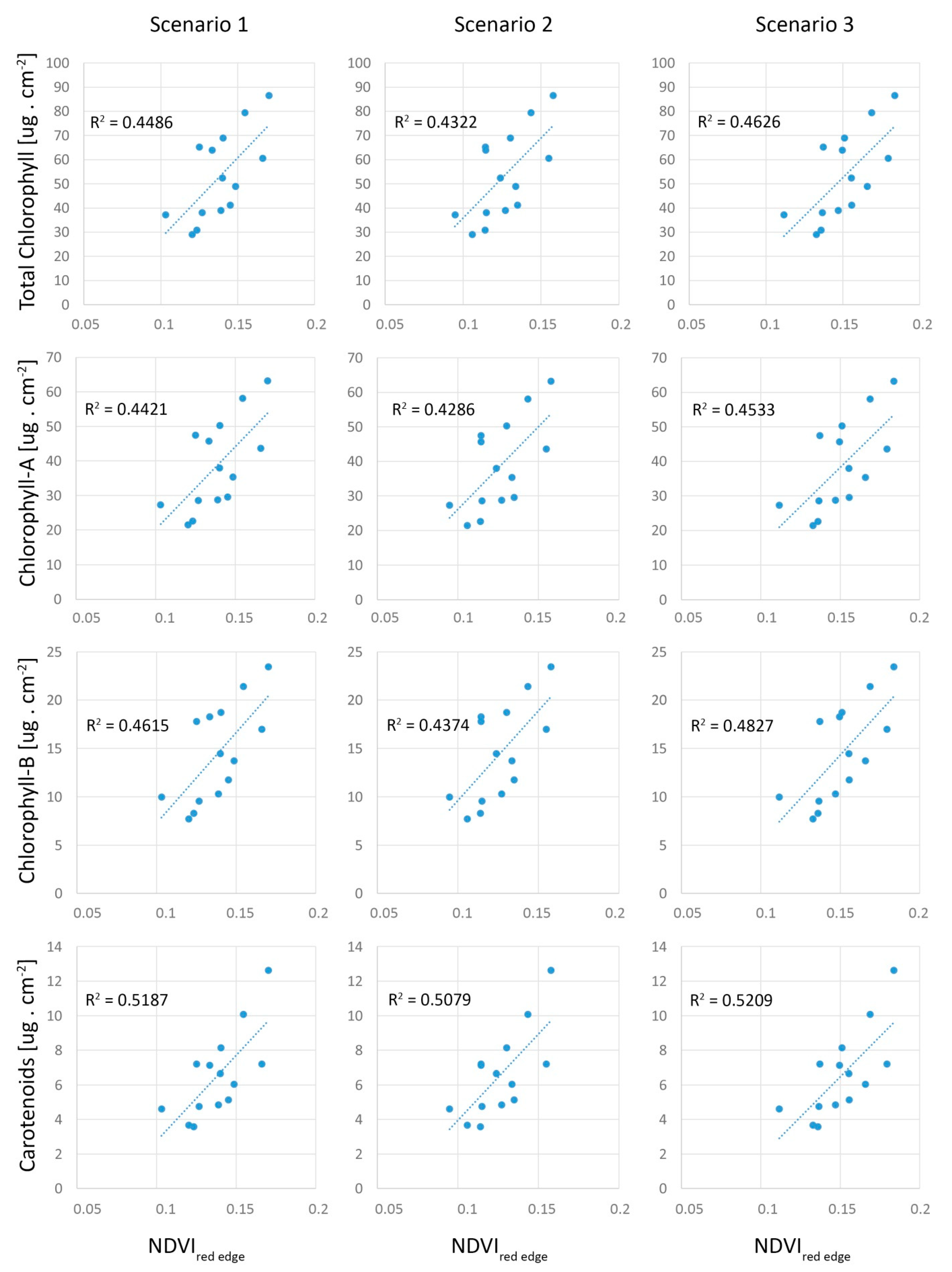
3.5. Relationship between Selected Vegetation Indexes and the Ground Truth

Both of the tested catchment areas were characterized by comparable NDVI_{red edge} values; however, a bigger difference in the NDVI values could be seen between the LYS and PLB catchments (

Table 9. Mean values/Standard deviations of vegetation indices based on Sequoia optical data per evaluated Scenarios for both catchments.

	Catchment	Scenario 1	Scenario 2	Scenario 3
NDVI	Lysina (LYS)	0.831/0.022	0.832/0.022	0.829/0.023
	Pluhův Bor (PLB)	0.782/0.056	0.772/0.055	0.770/0.059
NDVIred edge	Lysina (LYS)	0.138/0.022	0.130/0.019	0.149/0.025
	Pluhův Bor (PLB)	0.140/0.019	0.121/0.018	0.146/0.020

). In the methodological chapter (Section 2.5), three different scenarios were defined to assess the relationship between the spectral indices and photosynthetic pigments: Scenario 1: the whole crown (all pixels); Scenario 2: the top and the higher-illuminated part of the tree crown; and, Scenario 3: the lower-illuminated part of the tree crown. When comparing the results that were obtained for Scenarios 1–3 (Table 9, Figure 11), the NDVI index showed an almost negligible differences among all three Scenarios, while the NDVI_{red edge} index showed minimally larger differences among the defined scenarios.

The linear models were built between the VIs (NDVI and NDVI_{red edge}) and the ground truth (in-situ needle chlorophyll and carotenoid contents). The LYS 1K stand was identified as an outlier, as mentioned in Section 3.3. Besides the significant differences in tree age (Table 2), this stand was also characterized by a much higher tree density (field observations—LAI at LYS 1K = 4.47 in comparison to LYS 2K = 3.58 and LYS 4K = 3.70). High tree density indicated high VIs values; however, it did not correspond with rather low values of chlorophyll content. Therefore, LYS 1K was excluded from the further statistics. As a result, there were nine trees in total from the PLB catchment and six trees from the LYS catchment that were used for this statistical assessment. Three different scenarios were used (Figure 12 and Figure 13), for which the VIs were correlated with the ground truth (laboratory analysis of Chlorophyll a and b and carotenoids) using four different needle age groups too—all needles together included, first year needles included, second year needles included, and four year old needles included, as already described (

Table 10. Coefficients of determination (R²) for NDVI index and the four ground truth needle age groups.

Ground Truth Age Group	Parameter	Scenario 1	Scenario 2	Scenario 3
All needles	Total chlorophyll	0.33284	0.3132	0.34764
	Chlorophyll a	0.31794	0.30137	0.33012
	Chlorophyll b	0.36924	0.34138	0.39117
	Carotenoids	0.31854	0.2931	0.33969
1st year needles	Total chlorophyll	0.03731	0.04066	0.03605
	Chlorophyll a	0.03489	0.03854	0.03333
	Chlorophyll b	0.04373	0.04618	0.04336
	Carotenoids	0.07389	0.0579	0.08686
2nd year needles	Total chlorophyll	0.4801	0.44667	0.49043
	Chlorophyll A	0.47219	0.44141	0.48051
	Chlorophyll B	0.49659	0.45638	0.51224
	Carotenoids	0.48543	0.44873	0.50073
4th year needles	Total chlorophyll	0.21125	0.19238	0.23391
	Chlorophyll a	0.19768	0.18171	0.21753
	Chlorophyll b	0.24389	0.21744	0.27382
	Carotenoids	0.18607	0.16277	0.21334

Legend: .

and

Table 11. Coefficients of determination (R²) for NDVI_{red edge} index, and the four ground truth age groups.

Ground Truth Age Group	Parameter	Scenario 1	Scenario 2	Scenario 3
All needles	Total chlorophyll	0.33424	0.3367	0.32031
	Chlorophyll a	0.32371	0.32902	0.30735
	Chlorophyll b	0.35841	0.35316	0.35132
	Carotenoids	0.37654	0.37009	0.36017
1st year needles	Total chlorophyll	0.03079	0.05179	0.01875
	Chlorophyll a	0.03029	0.05143	0.0181
	Chlorophyll b	0.03195	0.05241	0.0181
	Carotenoids	0.07625	0.09464	0.07331
2nd year needles	Total chlorophyll	0.44861	0.43218	0.46261
	Chlorophyll a	0.44209	0.42862	0.45333
	Chlorophyll b	0.46151	0.43743	0.48268
	Carotenoids	0.51865	0.50788	0.52091
4th year needles	Total chlorophyll	0.2499	0.22732	0.24152
	Chlorophyll a	0.23973	0.22026	0.22884
	Chlorophyll b	0.27252	0.24211	0.27104
	Carotenoids	0.26164	0.23661	0.25304

Legend: .

). A similar pattern was identified, for both Vis. It can be concluded that the results differ significantly depending on what needle age group was used as ground truth. The worst results were obtained when the first year needle group was used (no correlation), followed by the four year old needle group and all age needle group used as ground truth (very weak correlation). On the other hand, for both VIs, the best results were obtained when the second year needle group was used as ground truth.

Assessing the different illumination crown conditions (Scenarios 1–3) in the case that the second year needle group was selected as ground truth (Table 10 and Table 11, Figure 12 and Figure 13), the worst results were surprisingly obtained for Scenario 2, where the top crown part receiving the higher-illumination was assessed, followed by Scenario 1—the whole crown case; the best results were obtained for Scenario 3—where the lower illumination part of the crown was assessed. For the NDVI index, the differences between Scenarios 1–3 are very small, slightly bigger differences could be found for the NDVI_{red edge} index. It can be concluded that the best results were achieved when the second year needle group was used as ground truth together with Scenario 3 for both VIs. Using this setting for the NDVI index, the following R² were obtained for photosynthetic pigments (Table 10): total chlorophyll—R² = 0.49, Chlorophyll a—R² = 0.48, Chlorophyll b—R² = 0.51, and Carotenoids—R² = 0.50. Comparable results were then also obtained for the NDVI_{red edge} index (Table 11): total chlorophyll—R² = 0.46, Chlorophyll a—R² = 0.45, Chlorophyll b—R² = 0.48, and Carotenoids—R² = 0.52. The NDVI index achieved a slightly higher R² for Total chlorophyll, Chlorophyll a and b contents, while NDVI_{red edge} showed slightly better results for Carotenoids.

4. Discussion

Regarding the first part of this analysis—tree height, crown, and top detection—it can be concluded that the obtained results satisfy the requirements of this study, which was basically aimed at identifying individual tree crowns and masking the background and shades. A relatively quick method was employed using Seq DSM and high resolution DEM (DMR 5G), and reliable results were obtained achieving R² = 0.90 and higher between CHM-estimated heights and the in-situ tree measurements for most of the stands, with the exception of PLB 2K (R² = 0.7) (Figure 9). The accuracy of tree-height estimation was comparable or even higher than in the case of Pinus ponderosa forest (R² = 0.71; [36]), where the same multispectral camera was used, although with a different type of UAV. The lower accuracy that was obtained for PLB 2K can be explained by changes happening between the time the in-situ data were collected (2015) and the UAV data acquisition (2018). In the field. it was observed that tree cuts were common in this particular forest stand. It will be interesting to test in the future, if this approach can be further employed or adjusted for estimating the forest aboveground biomass in a similar way as airborne laser scanning has been employed [62].

For both VIs a similar R² was obtained between the index values and the laboratory analysis of photosynthetic pigments, NDVI showed a slightly higher R² for chlorophyll content. while NDVI_{red edge} had the highest R² for carotenoid content. The Red edge is commonly used for detecting vegetation stress [93] and, in this study, it was also a slightly better index to estimate carotenoids—the vegetation stress indicators. The biggest influence on linear models for both was the selection of the needle age group used as a ground truth. As summarized in Table 10 and Table 11, basically the only usable results were obtained when using the second year needle pigment contents. The age-dependence of correlation strength between vegetation indices and measured pigment contents were expectable. However, the absence of a NDVI and NDVI_{red edge} correlation to chlorophyll and carotenoids for the first year needles was highly surprising. Such needles were already fully developed at the date of sampling (August 4-5th), thus the immaturity of needles as a likely reason was excluded. Moreover, first year needles are routinely and successfully used for taking ground truth for a broad range of spectroscopic and remote sensing studies at various scales from leaf- to stand level [89,93,94,95,96,97].

However, in some studies, second year needles, similarly as in this study, also proved to be the best option for predicting needle traits [60,98], although the physiological and optical causes have not been elucidated. The second year needles were also successfully used as ground truth for pigment content estimation from multispectral UAV data in mature Scots spine (Pinus sylvestris) [96]. The authors justified the selection of the second year needles, literally as “avoiding non-representative outliers in current and mature needles” [96]. The absence of correlation between chlorophyll content in first year needles and vegetation indices could be partly related to other interfering needle traits than chlorophyll content itself. Although water has absorption features in near- and shortwave infrared region, it sometimes shows an intercorrelation with chlorophyll content [99] and may influence its prediction from leaf spectral signal. The sampling year 2018 was rather dry and the water content in needles exhibited the opposite (increasing) trend towards older needles in comparison to previous season 2017 (Appendix A: Figure A2). We hypothesize that lower water content in 1st year needles could also negatively influence chlorophyll prediction from NDVI and NDVI_{red edge}. The effect of leaf water content on relationship among vegetation indices and leaf-level functional traits was observed in crops [100,101], however not yet confirmed for conifers.

In addition, this study’s results showed that first year needles exhibited the lowest chlorophyll contents (31–35 ug.cm², Table 4), and it can be hypothesized that such values, in combination with coniferous canopy structure, may be below the detection limit of the Parrot Sequoia multispectral camera. In a maize field case study [102], the authors concluded that hemispherical-conical reflectance factors, NDVI, and the chlorophyll red-edge index derived from the Sequoia sensor exhibit bias for high and low reflective surfaces. In comparison to broadleaf trees, conifer canopy NIR reflectance is generally lower [103] due to needle clustering within shoots and self-shading [104,105], and it is speculated that the needle photosynthetic pigment contents of the first year needles were, in this case, too low to be resolved by the Parrot Sequoia multispectral camera, which has limited spectral resolution and sensitivity as compared to hyperspectral sensors.

In this study, the crown light condition showed to be much less important than the needle age selection as a ground truth. Surprisingly the highest R² for both VIs was achieved when using the less sunlit, lower part of the crown (Scenario 3), followed by Scenario 1 (full crown) and then Scenario 2 (the more sun-lit top part of the crown). It seems that, at such a high spatial resolution, which was achieved when using the UAV platform, the tree structure and needle/branch position can cause these differences. The tree branches of the more sun-lit top part of the crown have a different position; they are shorter and more pointed up, while the less sunlit lower part of the crown has wider and flatter branches, thus the needles have a better position regarding the Sun, flight, and sensor geometry, as shown in Figure A3 (Appendix A). Additionally, the more sunlit top part of the crown is presented by a higher percentage of the first year needles, which were found to be problematic for the reasons that are discussed above. To date, the effect of heterogeneous light conditions within the crown on UAV-based leaf traits modelling was tested on broad leaved apple and pear trees with similar result to those in this study: the full canopy spectra provided, in some cases, more accurate models than only sunlit pixels [106]. The authors suggest that including the signal from the whole crown results in a bigger sample size, which may lead to model improvement. However, it can be concluded that very little is known about this issue and a complex study on reflectance variations regarding the tree/crown structure, needle configuration, and light conditions is still needed. It is also important to emphasize that no study was found to directly compare these results that were conducted on coniferous forest stands. This shows that building quantitative approaches employing Multi-spectral Unmanned Aerial Vehicle (UAV) images is still challenging for coniferous forests, in particular, those of natural origin. The number of the trees studied in this research was limited (18 trees). Follow up research is needed that would allow for extending the number of sampled trees to obtain generalizable results, especially for the regression models.

5. Conclusions

The results show that there is a big potential in using UAVs together with affordable multispectral cameras as a platform for monitoring forest status at a local scale, however, at high resolution. Tree crown delineation and derivation of other parameters, such as tree top and height, which was based on the Canopy Height Model (CHM) obtained from two data sources—digital surface model derived from the Parrot Sequoia camera multispectral images (Seq DSM) and high resolution Digital Elevation Model (DEM: DMR 5G), corresponded well with the in-situ data and it was satisfactory for the purposes of this study. The results of the conducted statistical analysis show that the two tested VIs (NDVI and NDVI_{red edge}) have the potential to assess photosynthetic pigments in Norway spruce forests at a semi-quantitative level; however, the selection of needle-age as a ground truth was revealed to be a very important factor. The only usable results were obtained for linear models when using the second year needle pigment contents as a ground truth.

On the other hand, the illumination conditions of the crown showed to have very little effect on the model’s validity, whereas slightly better results were obtained when assessing the less sunlit lower part of the crown, which is characterized by wider and more flat branches. When compared to the whole crown Scenario, the improvement was very small, and it is proposed that the whole part of the crown be used for simplicity. However, this effect might have a bigger impact on data with a very high spectral resolution (e.g., hyperspectral data), and further systematic research on reflectance variations regarding the tree/crown structure, needle configuration, and light conditions is still needed. No study was found, in which it was possible to directly compare these results conducted on coniferous (Norway spruce) forest stands; this shows that there is also a further need for studies dealing with a quantitative estimation of the biochemical variables of coniferous forests when employing spectral data that were acquired at the UAV platform at a very high spatial resolution.

References

1. Potapov, P.; Yaroshenko, A.; Turubanova, S.; Dubinin, M.; Laestadius, L.; Thies, C.; Aksenov, D.; Egorov, A.; Yesipova, Y.; Glushkov, I. Mapping the World’s Intact Forest Landscapes by Remote Sensing. Ecol. Soc. 2008, 13, 51. [Google Scholar] [CrossRef] [Green Version]
2. Boyd, D.S.; Danson, F.M. Satellite Remote Sensing of Forest Resources: Three Decades of Research Development. Prog. Phys. Geogr. 2005, 29, 1–26. [Google Scholar] [CrossRef]
3. De Vries, W.; Vel, E.; Reinds, G.J.; Deelstra, H.; Klap, J.M.; Leeters, E.; Hendriks, C.M.A.; Kerkvoorden, M.; Landmann, G.; Herkendell, J. Intensive Monitoring of Forest Ecosystems in Europe: 1. Objectives, Set-up and Evaluation Strategy. For. Ecol. Manag. 2003, 174, 77–95. [Google Scholar] [CrossRef]
4. Pause, M.; Schweitzer, C.; Rosenthal, M. In Situ/Remote Sensing Integration to Assess Forest Health—A Review. Remote Sens. 2016, 8, 471. [Google Scholar] [CrossRef] [Green Version]
5. Žibret, G.; Kopačková, V. Comparison of Two Methods for Indirect Measurement of Atmospheric Dust Deposition: Street-Dust Composition and Vegetation-Health Status Derived from Hyperspectral Image Data. Ambio 2019, 48, 423–435. [Google Scholar] [CrossRef]
6. Hruška, J.; Krám, P. Modelling Long-Term Changes in Stream Water and Soil Chemistry in Catchments with Contrasting Vulnerability to Acidification (Lysina and Pluhuv Bor, Czech Republic). Hydrol. Earth Syst. Sci. 2003, 7, 525–539. [Google Scholar] [CrossRef]
7. Švik, M.; Oulehle, F.; Krám, P.; Janoutová, R.; Tajovská, K.; Homolová, L. Landsat-Based Indices Reveal Consistent Recovery of Forested Stream Catchments from Acid Deposition. Remote Sens. 2020, 12, 1944. [Google Scholar] [CrossRef]
8. Fottová, D.; Skořepová, I. Changes in mass element fluxes and their importance for critical loads: GEOMON network, Czech Republic. In Biogeochemical Investigations at Watershed, Landscape, and Regional Scales; Springer: Berlin/Heidelberg, Germany, 1998; pp. 365–376. [Google Scholar]
9. Fottová, D. Trends in Sulphur and Nitrogen Deposition Fluxes in the GEOMON Network, Czech Republic, between 1994 and 2000. Water. Air. Soil Pollut. 2003, 150, 73–87. [Google Scholar] [CrossRef]
10. Oulehle, F.; Chuman, T.; Hruška, J.; Krám, P.; McDowell, W.H.; Myška, O.; Navrátil, T.; Tesař, M. Recovery from Acidification Alters Concentrations and Fluxes of Solutes from Czech Catchments. Biogeochemistry 2017, 132, 251–272. [Google Scholar] [CrossRef]
11. Krám, P.; Hruška, J.; Shanley, J.B. Streamwater Chemistry in Three Contrasting Monolithologic Czech Catchments. Appl. Geochem. 2012, 27, 1854–1863. [Google Scholar] [CrossRef]
12. Navrátil, T.; Kurz, D.; Krám, P.; Hofmeister, J.; Hruška, J. Acidification and Recovery of Soil at a Heavily Impacted Forest Catchment (Lysina, Czech Republic)—SAFE Modeling and Field Results. Ecol. Model. 2007, 205, 464–474. [Google Scholar] [CrossRef]
13. Oulehle, F.; McDowell, W.H.; Aitkenhead-Peterson, J.A.; Krám, P.; Hruška, J.; Navrátil, T.; Buzek, F.; Fottová, D. Long-Term Trends in Stream Nitrate Concentrations and Losses across Watersheds Undergoing Recovery from Acidification in the Czech Republic. Ecosystems 2008, 11, 410–425. [Google Scholar] [CrossRef]
14. dos Santos, A.A.; Junior, J.M.; Araújo, M.S.; Di Martini, D.R.; Tetila, E.C.; Siqueira, H.L.; Aoki, C.; Eltner, A.; Matsubara, E.T.; Pistori, H. Assessment of CNN-Based Methods for Individual Tree Detection on Images Captured by RGB Cameras Attached to UAVs. Sensors 2019, 19, 3595. [Google Scholar] [CrossRef] [Green Version]
15. Fujimoto, A.; Haga, C.; Matsui, T.; Machimura, T.; Hayashi, K.; Sugita, S.; Takagi, H. An End to End Process Development for UAV-SfM Based Forest Monitoring: Individual Tree Detection, Species Classification and Carbon Dynamics Simulation. Forests 2019, 10, 680. [Google Scholar] [CrossRef] [Green Version]
16. Fayad, I.; Baghdadi, N.; Guitet, S.; Bailly, J.-S.; Hérault, B.; Gond, V.; El Hajj, M.; Minh, D.H.T. Aboveground Biomass Mapping in French Guiana by Combining Remote Sensing, Forest Inventories and Environmental Data. Int. J. Appl. Earth Obs. Geoinform. 2016, 52, 502–514. [Google Scholar] [CrossRef] [Green Version]
17. White, J.C.; Coops, N.C.; Wulder, M.A.; Vastaranta, M.; Hilker, T.; Tompalski, P. Remote Sensing Technologies for Enhancing Forest Inventories: A Review. Can. J. Remote Sens. 2016, 42, 619–641. [Google Scholar] [CrossRef] [Green Version]
18. Masek, J.G.; Hayes, D.J.; Hughes, M.J.; Healey, S.P.; Turner, D.P. The Role of Remote Sensing in Process-Scaling Studies of Managed Forest Ecosystems. For. Ecol. Manag. 2015, 355, 109–123. [Google Scholar] [CrossRef] [Green Version]
19. Lausch, A.; Heurich, M.; Gordalla, D.; Dobner, H.-J.; Gwillym-Margianto, S.; Salbach, C. Forecasting Potential Bark Beetle Outbreaks Based on Spruce Forest Vitality Using Hyperspectral Remote-Sensing Techniques at Different Scales. For. Ecol. Manag. 2013, 308, 76–89. [Google Scholar] [CrossRef]
20. Halme, E.; Pellikka, P.; Mõttus, M. Utility of Hyperspectral Compared to Multispectral Remote Sensing Data in Estimating Forest Biomass and Structure Variables in Finnish Boreal Forest. Int. J. Appl. Earth Obs. Geoinform. 2019, 83, 101942. [Google Scholar] [CrossRef]
21. Jarocińska, A.; Białczak, M.; Sławik, Ł. Application of Aerial Hyperspectral Images in Monitoring Tree Biophysical Parameters in Urban Areas. Misc. Geogr. 2018, 22, 56–62. [Google Scholar] [CrossRef] [Green Version]
22. Kopačková, V.; Mišurec, J.; Lhotáková, Z.; Oulehle, F.; Albrechtová, J. Using Multi-Date High Spectral Resolution Data to Assess the Physiological Status of Macroscopically Undamaged Foliage on a Regional Scale. Int. J. Appl. Earth Obs. Geoinform. 2014, 27, 169–186. [Google Scholar] [CrossRef]
23. Machala, M.; Zejdová, L. Forest Mapping Through Object-Based Image Analysis of Multispectral and LiDAR Aerial Data. Eur. J. Remote Sens. 2014, 47, 117–131. [Google Scholar] [CrossRef]
24. Mišurec, J.; Kopačková, V.; Lhotáková, Z.; Campbell, P.; Albrechtová, J. Detection of Spatio-Temporal Changes of Norway Spruce Forest Stands in Ore Mountains Using Landsat Time Series and Airborne Hyperspectral Imagery. Remote Sens. 2016, 8, 92. [Google Scholar] [CrossRef] [Green Version]
25. Lin, Y.; Jiang, M.; Yao, Y.; Zhang, L.; Lin, J. Use of UAV Oblique Imaging for the Detection of Individual Trees in Residential Environments. Urban For. Urban Green. 2015, 14, 404–412. [Google Scholar] [CrossRef]
26. Klein Hentz, Â.M.; Corte, A.P.D.; Péllico Netto, S.; Strager, M.P.; Schoeninger, E.R. Treedetection: Automatic Tree Detection Using UAV-Based Data. Floresta 2018, 48, 393. [Google Scholar] [CrossRef]
27. Candiago, S.; Remondino, F.; De Giglio, M.; Dubbini, M.; Gattelli, M. Evaluating Multispectral Images and Vegetation Indices for Precision Farming Applications from UAV Images. Remote Sens. 2015, 7, 4026–4047. [Google Scholar] [CrossRef] [Green Version]
28. Sona, G.; Passoni, D.; Pinto, L.; Pagliari, D.; Masseroni, D.; Ortuani, B.; Facchi, A. UAV Multispectral Survey to Map Soil and Crop for Precision Farming Applications. ISPRS Int. Arch. Photogramm. Remote Sens. Spat. Inf. Sci. 2016, 1023–1029. [Google Scholar] [CrossRef] [Green Version]
29. Albetis, J.; Duthoit, S.; Guttler, F.; Jacquin, A.; Goulard, M.; Poilvé, H.; Féret, J.-B.; Dedieu, G. Detection of Flavescence Dorée Grapevine Disease Using Unmanned Aerial Vehicle (UAV) Multispectral Imagery. Remote Sens. 2017, 9, 308. [Google Scholar] [CrossRef] [Green Version]
30. Su, J.; Liu, C.; Hu, X.; Xu, X.; Guo, L.; Chen, W.-H. Spatio-Temporal Monitoring of Wheat Yellow Rust Using UAV Multispectral Imagery. Comput. Electron. Agric. 2019, 167, 105035. [Google Scholar] [CrossRef]
31. Singhal, G.; Bansod, B.; Mathew, L.; Goswami, J.; Choudhury, B.U.; Raju, P.L.N. Chlorophyll Estimation Using Multi-Spectral Unmanned Aerial System Based on Machine Learning Techniques. Remote Sens. Appl. Soc. Environ. 2019, 15, 100235. [Google Scholar] [CrossRef]
32. Guo, Y.; Wang, H.; Wu, Z.; Wang, S.; Sun, H.; Senthilnath, J.; Wang, J.; Robin Bryant, C.; Fu, Y. Modified Red Blue Vegetation Index for Chlorophyll Estimation and Yield Prediction of Maize from Visible Images Captured by UAV. Sensors 2020, 20, 5055. [Google Scholar] [CrossRef] [PubMed]
33. Baluja, J.; Diago, M.P.; Balda, P.; Zorer, R.; Meggio, F.; Morales, F.; Tardaguila, J. Assessment of Vineyard Water Status Variability by Thermal and Multispectral Imagery Using an Unmanned Aerial Vehicle (UAV). Irrig. Sci. 2012, 30, 511–522. [Google Scholar] [CrossRef]
34. Turner, D.; Lucieer, A.; Watson, C. Development of an Unmanned Aerial Vehicle (UAV) for Hyper Resolution Vineyard Mapping Based on Visible, Multispectral, and Thermal Imagery. In Proceedings of the 34th International Symposium on Remote Sensing of Environment, Sydney, NSW, Australia, 10–15 April 2011; p. 4. [Google Scholar]
35. Zarco-Tejada, P.J.; Guillén-Climent, M.L.; Hernández-Clemente, R.; Catalina, A.; González, M.R.; Martín, P. Estimating Leaf Carotenoid Content in Vineyards Using High Resolution Hyperspectral Imagery Acquired from an Unmanned Aerial Vehicle (UAV). Agric. For. Meteorol. 2013, 171–172, 281–294. [Google Scholar] [CrossRef] [Green Version]
36. Belmonte, A.; Sankey, T.; Biederman, J.A.; Bradford, J.; Goetz, S.J.; Kolb, T.; Woolley, T. UAV-derived Estimates of Forest Structure to Inform Ponderosa Pine Forest Restoration. Remote Sens. Ecol. Conserv. 2020, 6, 181–197. [Google Scholar] [CrossRef]
37. D’Odorico, P.; Besik, A.; Wong, C.Y.S.; Isabel, N.; Ensminger, I. High-throughput Drone-based Remote Sensing Reliably Tracks Phenology in Thousands of Conifer Seedlings. New Phytol. 2020, 226, 1667–1681. [Google Scholar] [CrossRef] [PubMed]
38. Dash, J.P.; Watt, M.S.; Pearse, G.D.; Heaphy, M.; Dungey, H.S. Assessing Very High Resolution UAV Imagery for Monitoring Forest Health during a Simulated Disease Outbreak. ISPRS J. Photogramm. Remote Sens. 2017, 131, 1–14. [Google Scholar] [CrossRef]
39. Chianucci, F.; Disperati, L.; Guzzi, D.; Bianchini, D.; Nardino, V.; Lastri, C.; Rindinella, A.; Corona, P. Estimation of Canopy Attributes in Beech Forests Using True Colour Digital Images from a Small Fixed-Wing UAV. Int. J. Appl. Earth Obs. Geoinform. 2016, 47, 60–68. [Google Scholar] [CrossRef] [Green Version]
40. Dash, J.; Pearse, G.; Watt, M. UAV Multispectral Imagery Can Complement Satellite Data for Monitoring Forest Health. Remote Sens. 2018, 10, 1216. [Google Scholar] [CrossRef] [Green Version]
41. Minařík, R.; Langhammer, J. Use of a Multispectral UAV Photogrammetry for Detection and Tracking of Forest Disturbance Dynamics. ISPRS Int. Arch. Photogramm. Remote Sens. Spat. Inf. Sci. 2016, 711–718. [Google Scholar] [CrossRef]
42. Franklin, S.E. Pixel- and Object-Based Multispectral Classification of Forest Tree Species from Small Unmanned Aerial Vehicles. J. Unmanned Veh. Syst. 2018, 6, 195–211. [Google Scholar] [CrossRef] [Green Version]
43. Näsi, R.; Honkavaara, E.; Lyytikäinen-Saarenmaa, P.; Blomqvist, M.; Litkey, P.; Hakala, T.; Viljanen, N.; Kantola, T.; Tanhuanpää, T.; Holopainen, M. Using UAV-Based Photogrammetry and Hyperspectral Imaging for Mapping Bark Beetle Damage at Tree-Level. Remote Sens. 2015, 7, 15467–15493. [Google Scholar] [CrossRef] [Green Version]
44. Berveglieri, A.; Tommaselli, A.M.G. Exterior Orientation of Hyperspectral Frame Images Collected with UAV for Forest Applications. ISPRS Int. Arch. Photogramm. Remote Sens. Spat. Inf. Sci. 2016, 40, 45–50. [Google Scholar] [CrossRef] [Green Version]
45. Gallardo-Salazar, J.L.; Pompa-García, M. Detecting Individual Tree Attributes and Multispectral Indices Using Unmanned Aerial Vehicles: Applications in a Pine Clonal Orchard. Remote Sens. 2020, 12, 4144. [Google Scholar] [CrossRef]
46. Lim, Y.S.; La, P.H.; Park, J.S.; Lee, M.H.; Pyeon, M.W.; Kim, J.-I. Calculation of Tree Height and Canopy Crown from Drone Images Using Segmentation. J. Kor. Soc. Survey. Geodesy Photogram. Cartogr. 2015, 33, 605–614. [Google Scholar] [CrossRef] [Green Version]
47. Díaz-Varela, R.; de la Rosa, R.; León, L.; Zarco-Tejada, P. High-Resolution Airborne UAV Imagery to Assess Olive Tree Crown Parameters Using 3D Photo Reconstruction: Application in Breeding Trials. Remote Sens. 2015, 7, 4213–4232. [Google Scholar] [CrossRef] [Green Version]
48. Wu, X.; Shen, X.; Cao, L.; Wang, G.; Cao, F. Assessment of Individual Tree Detection and Canopy Cover Estimation Using Unmanned Aerial Vehicle Based Light Detection and Ranging (UAV-LiDAR) Data in Planted Forests. Remote Sens. 2019, 11, 908. [Google Scholar] [CrossRef] [Green Version]
49. Panagiotidis, D.; Abdollahnejad, A.; Surový, P.; Chiteculo, V. Determining Tree Height and Crown Diameter from High-Resolution UAV Imagery. Int. J. Remote Sens. 2017, 38, 2392–2410. [Google Scholar] [CrossRef]
50. Jaakkola, A.; Hyyppä, J.; Yu, X.; Kukko, A.; Kaartinen, H.; Liang, X.; Hyyppä, H.; Wang, Y. Autonomous Collection of Forest Field Reference—The Outlook and a First Step with UAV Laser Scanning. Remote Sens. 2017, 9, 785. [Google Scholar] [CrossRef] [Green Version]
51. Silva, C.A.; Crookston, N.L.; Hudak, A.T.; Vierling, L.A.; Klauberg, C.; Cardil, A. RLiDAR: LiDAR Data Processing and Visualization; The R Foundation: Vienna, Austria, 2017. [Google Scholar]
52. Cardil, A.; Otsu, K.; Pla, M.; Silva, C.A.; Brotons, L. Quantifying Pine Processionary Moth Defoliation in a Pine-Oak Mixed Forest Using Unmanned Aerial Systems and Multispectral Imagery. PLoS ONE 2019, 14, e0213027. [Google Scholar] [CrossRef]
53. Zaforemska, A.; Xiao, W.; Gaulton, R. Individual Tree Detection from UAV LIDAR Data in a Mixed Species Woodland. ISPRS Int. Arch. Photogramm. Remote Sens. Spat. Inf. Sci. 2019, 657–663. [Google Scholar] [CrossRef] [Green Version]
54. Li, J.; Yang, B.; Cong, Y.; Cao, L.; Fu, X.; Dong, Z. 3D Forest Mapping Using A Low-Cost UAV Laser Scanning System: Investigation and Comparison. Remote Sens. 2019, 11, 717. [Google Scholar] [CrossRef] [Green Version]
55. Kuželka, K.; Slavík, M.; Surový, P. Very High Density Point Clouds from UAV Laser Scanning for Automatic Tree Stem Detection and Direct Diameter Measurement. Remote Sens. 2020, 12, 1236. [Google Scholar] [CrossRef] [Green Version]
56. Picos, J.; Bastos, G.; Míguez, D.; Alonso, L.; Armesto, J. Individual Tree Detection in a Eucalyptus Plantation Using Unmanned Aerial Vehicle (UAV)-LiDAR. Remote Sens. 2020, 12, 885. [Google Scholar] [CrossRef] [Green Version]
57. Pulido, D.; Salas, J.; Rös, M.; Puettmann, K.; Karaman, S. Assessment of Tree Detection Methods in Multispectral Aerial Images. Remote Sens. 2020, 12, 2379. [Google Scholar] [CrossRef]
58. Pleșoianu, A.-I.; Stupariu, M.-S.; Șandric, I.; Pătru-Stupariu, I.; Drăguț, L. Individual Tree-Crown Detection and Species Classification in Very High-Resolution Remote Sensing Imagery Using a Deep Learning Ensemble Model. Remote Sens. 2020, 12, 2426. [Google Scholar] [CrossRef]
59. Fromm, M.; Schubert, M.; Castilla, G.; Linke, J.; McDermid, G. Automated Detection of Conifer Seedlings in Drone Imagery Using Convolutional Neural Networks. Remote Sens. 2019, 11, 2585. [Google Scholar] [CrossRef] [Green Version]
60. Lhotáková, Z.; Kopačková-Strnadová, V.; Oulehle, F.; Homolová, L.; Neuwirthová, E.; Švik, M.; Janoutová, R.; Albrechtová, J. Foliage Biophysical Trait Prediction from Laboratory Spectra in Norway Spruce Is More Affected by Needle Age Than by Site Soil Conditions. Remote Sens. 2021, 13, 391. [Google Scholar] [CrossRef]
61. ČÚZK: Geoportál. Available online: https://geoportal.cuzk.cz/(S(5rmwjwtpueumnrsepeeaarwk))/Default.aspx?head_tab=sekce-00-gp&mode=TextMeta&text=uvod_uvod&menu=01&news=yes&UvodniStrana=yes (accessed on 31 December 2020).
62. Novotný, J.; Navrátilová, B.; Janoutová, R.; Oulehle, F.; Homolová, L. Influence of Site-Specific Conditions on Estimation of Forest above Ground Biomass from Airborne Laser Scanning. Forests 2020, 11, 268. [Google Scholar] [CrossRef] [Green Version]
63. Porra, R.J.; Thompson, W.A.; Kriedemann, P.E. Determination of Accurate Extinction Coefficients and Simultaneous Equations for Assaying Chlorophylls a and b Extracted with Four Different Solvents: Verification of the Concentration of Chlorophyll Standards by Atomic Absorption Spectroscopy. Biochim. Biophys. Acta BBA Bioenerg. 1989, 975, 384–394. [Google Scholar] [CrossRef]
64. Wellburn, A.R. The Spectral Determination of Chlorophylls a and b, as Well as Total Carotenoids, Using Various Solvents with Spectrophotometers of Different Resolution. J. Plant Physiol. 1994, 144, 307–313. [Google Scholar] [CrossRef]
65. DJI—Official Website. Available online: https://www.dji.com (accessed on 30 December 2020).
66. Phantom 4—DJI. Available online: https://www.dji.com/phantom-4 (accessed on 30 December 2020).
67. SenseFly—SenseFly—The Professional’s Mapping Drone. Available online: https://www.sensefly.com/ (accessed on 30 December 2020).
68. Prusa3D—Open-Source 3D Printers from Josef Prusa. Available online: https://www.prusa3d.com/ (accessed on 30 December 2020).
69. Litchi for DJI Mavic/Phantom/Inspire/Spark. Available online: https://flylitchi.com/ (accessed on 31 December 2020).
70. Best Practices: Collecting Data with MicaSense Sensors. Available online: https://support.micasense.com/hc/en-us/articles/224893167-Best-practices-Collecting-Data-with-MicaSense-Sensors (accessed on 31 December 2020).
71. Agisoft Metashape. Available online: https://www.agisoft.com/ (accessed on 31 December 2020).
72. Westoby, M.J.; Brasington, J.; Glasser, N.F.; Hambrey, M.; Reynolds, J.M. ‘Structure-from-Motion’ Photogrammetry: A Low-Cost, Effective Tool for Geoscience Applications. Geomorphology 2012, 179, 300–314. [Google Scholar] [CrossRef] [Green Version]
73. Tutorial (Intermediate Level): Radiometric Calibration Using Reflectance Panelsin PhotoScan Professional 1.4. Available online: https://www.agisoft.com/pdf/PS_1.4_(IL)_Refelctance_Calibration.pdf (accessed on 20 December 2020).
74. Zhao, K.; Popescu, S. Hierarchical Watershed Segmentation of Canopy Height Model for Multi-Scale Forest Inventory. In Proceedings of the ISPRS working group “Laser Scanning 2007 and SilviLaser 2007”, Espoo, Finland, 12–14 September 2007; pp. 436–440. [Google Scholar]
75. Hubacek, M.; Kovarik, V.; Kratochvil, V. Analysis of Influence of Terrain Relief Roughness on DEM Accuracy Generated from LIDAR in the Czech Republic Territory. In Proceedings of the ISPRS—International Archives of the Photogrammetry, Remote Sensing and Spatial Information Sciences, Prague, Czech Republic, 12–19 July 2016; Copernicus GmbH: Göttingen, Germany; Volume XLI-B4, pp. 25–30. [Google Scholar]
76. How Focal Statistics Works—Help|ArcGIS for Desktop. Available online: https://desktop.arcgis.com/en/arcmap/10.3/tools/spatial-analyst-toolbox/how-focal-statistics-works.htm (accessed on 31 December 2020).
77. Xu, N.; Tian, J.; Tian, Q.; Xu, K.; Tang, S. Analysis of Vegetation Red Edge with Different Illuminated/Shaded Canopy Proportions and to Construct Normalized Difference Canopy Shadow Index. Remote Sens. 2019, 11, 1192. [Google Scholar] [CrossRef] [Green Version]
78. Rouse, J.W.; Hass, R.H.; Schell, J.A.; Deering, D.W.; Harlan, J.C. Monitoring the Vernal Advancement and Retrogradation (Green Wave Effect) of Natural Vegetation.; RSC 1978-4; Texas A & M University: College Station, TX, USA, 1974. [Google Scholar]
79. Sharma, L.; Bu, H.; Denton, A.; Franzen, D. Active-Optical Sensors Using Red NDVI Compared to Red Edge NDVI for Prediction of Corn Grain Yield in North Dakota, U.S.A. Sensors 2015, 15, 27832–27853. [Google Scholar] [CrossRef] [PubMed]
80. Gitelson, A.; Merzlyak, M.N. Spectral Reflectance Changes Associated with Autumn Senescence of Aesculus Hippocastanum L. and Acer Platanoides L. Leaves. Spectral Features and Relation to Chlorophyll Estimation. J. Plant Physiol. 1994, 143, 286–292. [Google Scholar] [CrossRef]
81. Sims, D.A.; Gamon, J.A. Relationships between Leaf Pigment Content and Spectral Reflectance across a Wide Range of Species, Leaf Structures and Developmental Stages. Remote Sens. Environ. 2002, 81, 337–354. [Google Scholar] [CrossRef]
82. Chavez, P.S., Jr.; Kwarteng, A.Y. Extracting Spectral Contrast in Landsat Thematic Mapper Image Data Using Selective Principal Component Analysis. Photogramm. Eng. Remote Sens. 1989, 55, 10. [Google Scholar]
83. Mather, P.M.; Koch, M. Computer Processing of Remotely-Sensed Images: An Introduction, 4th ed.; Wiley-Blackwell: Chichester, UK; Hoboken, NJ, USA, 2011; ISBN 978-0-470-74239-6. [Google Scholar]
84. Draper, N.R.; Smith, H. Applied Regression Analysis. In Wiley Series in Probability and Statistics, 1st ed.; Wiley: Hoboken, NJ, USA, 1998; ISBN 978-0-471-17082-2. [Google Scholar]
85. Homolová, L.; Lukeš, P.; Malenovský, Z.; Lhotáková, Z.; Kaplan, V.; Hanuš, J. Measurement Methods and Variability Assessment of the Norway Spruce Total Leaf Area: Implications for Remote Sensing. Trees 2013, 27, 111–121. [Google Scholar] [CrossRef] [Green Version]
86. Krám, P.; Oulehle, F.; Štědrá, V.; Hruška, J.; Shanley, J.B.; Minocha, R.; Traister, E. Geoecology of a Forest Watershed Underlain by Serpentine in Central Europe. Northeast. Nat. 2009, 16, 309–328. [Google Scholar] [CrossRef]
87. O’Neill, A.L.; Kupiec, J.A.; Curran, P.J. Biochemical and Reflectance Variation throughout a Sitka Spruce Canopy. Remote Sens. Environ. 2002, 80, 134–142. [Google Scholar] [CrossRef]
88. Hovi, A.; Raitio, P.; Rautiainen, M. A Spectral Analysis of 25 Boreal Tree Species. Silva Fenn. 2017, 51. [Google Scholar] [CrossRef] [Green Version]
89. Rautiainen, M.; Lukeš, P.; Homolová, L.; Hovi, A.; Pisek, J.; Mõttus, M. Spectral Properties of Coniferous Forests: A Review of In Situ and Laboratory Measurements. Remote Sens. 2018, 10, 207. [Google Scholar] [CrossRef] [Green Version]
90. Wu, Q.; Song, C.; Song, J.; Wang, J.; Chen, S.; Yu, B. Impacts of Leaf Age on Canopy Spectral Signature Variation in Evergreen Chinese Fir Forests. Remote Sens. 2018, 10, 262. [Google Scholar] [CrossRef] [Green Version]
91. Rogers, S.R.; Manning, I.; Livingstone, W. Comparing the Spatial Accuracy of Digital Surface Models from Four Unoccupied Aerial Systems: Photogrammetry Versus LiDAR. Remote Sens. 2020, 12, 2806. [Google Scholar] [CrossRef]
92. Zhang, L.; Sun, X.; Wu, T.; Zhang, H. An analysis of shadow effects on spectral vegetation indexes using a ground-based imaging spectrometer. IEEE Geosci. Remote Sens. Lett. 2015, 12, 2188–2192. [Google Scholar] [CrossRef]
93. Rock, B.N.; Hoshizaki, T.; Miller, J.R. Comparison of in Situ and Airborne Spectral Measurements of the Blue Shift Associated with Forest Decline. Remote Sens. Environ. 1988, 24, 109–127. [Google Scholar] [CrossRef]
94. Campbell, P.K.E.; Rock, B.N.; Martin, M.E.; Neefus, C.D.; Irons, J.R.; Middleton, E.M.; Albrechtova, J. Detection of Initial Damage in Norway Spruce Canopies Using Hyperspectral Airborne Data. Int. J. Remote Sens. 2004, 25, 5557–5584. [Google Scholar] [CrossRef]
95. de Tomás Marín, S.; Novák, M.; Klančnik, K.; Gaberščik, A. Spectral Signatures of Conifer Needles Mainly Depend on Their Physical Traits. Pol. J. Ecol. 2016, 64, 1–13. [Google Scholar] [CrossRef]
96. Misurec, J.; Kopacková, V.; Lhotakova, Z.; Albrechtova, J.; Hanus, J.; Weyermann, J.; Entcheva-Campbell, P. Utilization of Hyperspectral Image Optical Indices to Assess the Norway Spruce Forest Health Status. J. Appl. Remote Sens. 2012, 6, 063545. [Google Scholar] [CrossRef]
97. Hernández-Clemente, R.; Navarro-Cerrillo, R.M.; Zarco-Tejada, P.J. Carotenoid Content Estimation in a Heterogeneous Conifer Forest Using Narrow-Band Indices and PROSPECT+DART Simulations. Remote Sens. Environ. 2012, 127, 298–315. [Google Scholar] [CrossRef]
98. Kováč, D.; Malenovský, Z.; Urban, O.; Špunda, V.; Kalina, J.; Ač, A.; Kaplan, V.; Hanuš, J. Response of Green Reflectance Continuum Removal Index to the Xanthophyll De-Epoxidation Cycle in Norway Spruce Needles. J. Exp. Bot. 2013, 64, 1817–1827. [Google Scholar] [CrossRef] [PubMed] [Green Version]
99. Kokaly, R.F.; Asner, G.P.; Ollinger, S.V.; Martin, M.E.; Wessman, C.A. Characterizing Canopy Biochemistry from Imaging Spectroscopy and Its Application to Ecosystem Studies. Remote Sens. Environ. 2009, 113, S78–S91. [Google Scholar] [CrossRef]
100. Klem, K.; Záhora, J.; Zemek, F.; Trunda, P.; Tůma, I.; Novotná, K.; Hodaňová, K.; Rapantová, B.; Hanuš, J.; Vaříková, J.; et al. Interactive effects of water deficit and nitrogen nutrition on winter wheat. Remote sensing methods for their detection. Agricult. Water Manag. 2018, 210, 171–184. [Google Scholar] [CrossRef]
101. Schlemmer, M.R.; Francis, D.D.; Shanahan, J.F.; Schepers, J.S. Remotely measuring chlorophyll content in corn leaves with differing nitrogen levels and relative water content. Agron. J. 2005, 97, 106–112. [Google Scholar] [CrossRef] [Green Version]
102. Fawcett, D.; Panigada, C.; Tagliabue, G.; Boschetti, M.; Celesti, M.; Evdokimov, A.; Biriukova, K.; Colombo, R.; Miglietta, F.; Rascher, U.; et al. Multi-Scale Evaluation of Drone-Based Multispectral Surface Reflectance and Vegetation Indices in Operational Conditions. Remote Sens. 2020, 12, 514. [Google Scholar] [CrossRef] [Green Version]
103. Ollinger, S.V. Sources of Variability in Canopy Reflectance and the Convergent Properties of Plants: Tansley Review. New Phytol. 2011, 189, 375–394. [Google Scholar] [CrossRef]
104. Cescatti, A.; Zorer, R. Structural Acclimation and Radiation Regime of Silver Fir (Abies Alba Mill.) Shoots along a Light Gradient: Shoot Structure and Radiation Regime. Plant Cell Environ. 2003, 26, 429–442. [Google Scholar] [CrossRef]
105. Kubínová, Z.; Janáček, J.; Lhotáková, Z.; Šprtová, M.; Kubínová, L.; Albrechtová, J. Norway Spruce Needle Size and Cross Section Shape Variability Induced by Irradiance on a Macro- and Microscale and CO2 Concentration. Trees 2018, 32, 231–244. [Google Scholar] [CrossRef]
106. Vanbrabant, Y.; Tits, L.; Delalieux, S.; Pauly, K.; Verjans, W.; Somers, B. Multitemporal Chlorophyll Mapping in Pome Fruit Orchards from Remotely Piloted Aircraft Systems. Remote Sens. 2019, 11, 1468. [Google Scholar] [CrossRef] [Green Version]
Figure 1. Location of the test sites Pluhův Bor and Lysina in the Czech Republic, Europe: (a) the test sites displayed on a map of the Czech Republic; (b) maps of the Lysina and Pluhův Bor catchments with tree stands highlighted; an Orthophoto of the Czech Republic in the background [61].
Remotesensing 13 00705 g001
Figure 2. Unmanned Aerial Vehicle (UAV) equipment used in this study: (a) three-dimensional (3D) models of the mounts designed for the Parrot Sequoia multispectral camera; (b) DJI Phantom 4 quadcopter with attached Parrot Sequoia camera; and, (c) planned flight path in the flylitchi.com web tool.
Remotesensing 13 00705 g002
Figure 3. Workflow used in this study to detect tree height, crown and top.
Remotesensing 13 00705 g003
Figure 4. An example of tree crown detection (tree peaks visualized by green dots): (a) watersheds surrounding treetops (white line) split nearby trees—the borders are highlighted in red; DSM on the background; (b) the height mask (yellow line) cuts one side of the tree crowns in a place with a high altitude difference (red highlight); (c) the shadow mask (orange line) reduces the dark parts of tree crowns and completes the tree crown borders; multispectral imagery from the Parrot Sequoia sensor on the background (false-colour composition: Green, Red, Red edge); and, (d) final result of tree crown detection.
Remotesensing 13 00705 g004
Figure 5. Parrot Sequoia multispectral data processing workflow chart.
Remotesensing 13 00705 g005
Figure 6. Example (LYS 2K) of the UAV survey products used in this study: (a) the RGB orthomosaic obtained from the DJI camera; (b) the multispectral mosaic derived from the Parrot Sequoia sensor (false-colour composition: Green, Red, Red edge); and, (c) the digital surface models (DSM) derived from the Parrot Sequoia multispectral data.
Remotesensing 13 00705 g006
Figure 7. Example of result data from tree peak, height and crown detection process: (a) LYS 1K test location; (b) LYS 2K test location. Green dots represent estimated tree peaks, yellow polygons delineate detected tree crowns and red-line polygons show the three trees at each stand which were sampled for photosynthetic pigment contents. The background image is the Multispectral Parrot Sequoia mosaic (false-colour composition: Green, Red, Red edge).
Remotesensing 13 00705 g007
Figure 8. Tree height distribution visualized by box plots. Blue boxes represent trees detected by the automatic algorithm from UAV-based CHM data (2018) and orange boxes display the distribution of the tree heights measured in-situ in 2015.
Remotesensing 13 00705 g008
Figure 9. Linear regression and coefficients of determination (R2): the CHM-estimated heights of the 20 highest trees at each stand compared to the in-situ data.
Remotesensing 13 00705 g009
Figure 10. Scheme of Tree No. 22 at the PLB 5K stand showing (a) Parrot Sequoia multispectral data in band combination 4-2-1 (NIR, Red, Green) corresponding to Scenario 1; (b) two classes representing Scenario 2 (the top higher-illumination part of the crown) and Scenario 3 (the lower-illumination part of the crown); and, (c) mean reflectance per two illumination scenarios. Vertical bars represent minimum and maximum values for each band and scenario.
Remotesensing 13 00705 g010
Figure 11. Normalized Difference Vegetation Index (NDVI), NDVIred edge: mean value and standard deviation for two illumination Scenarios 2 and 3 (summarized for each catchment area).
Remotesensing 13 00705 g011
Figure 12. Linear regression between NDVI index and second year needles photosynthetic pigment content for Scenarios 1–3.
Remotesensing 13 00705 g012
Figure 13. Linear regression between NDVIred edge index and second year needles’ photosynthetic pigment content for Scenarios 1–3.
Remotesensing 13 00705 g013