Laser Scanning Based Surface Flatness Measurement Using Flat Mirrors for Enhancing Scan Coverage Range


Abstract
1. Introduction
2. Research Background
2.1. Current Practices for Surface Flatness Inspection
2.2. Surface Flatness Inspection Methods Using TLS
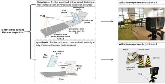
3. Research Hypotheses
4. Experimental Configuration
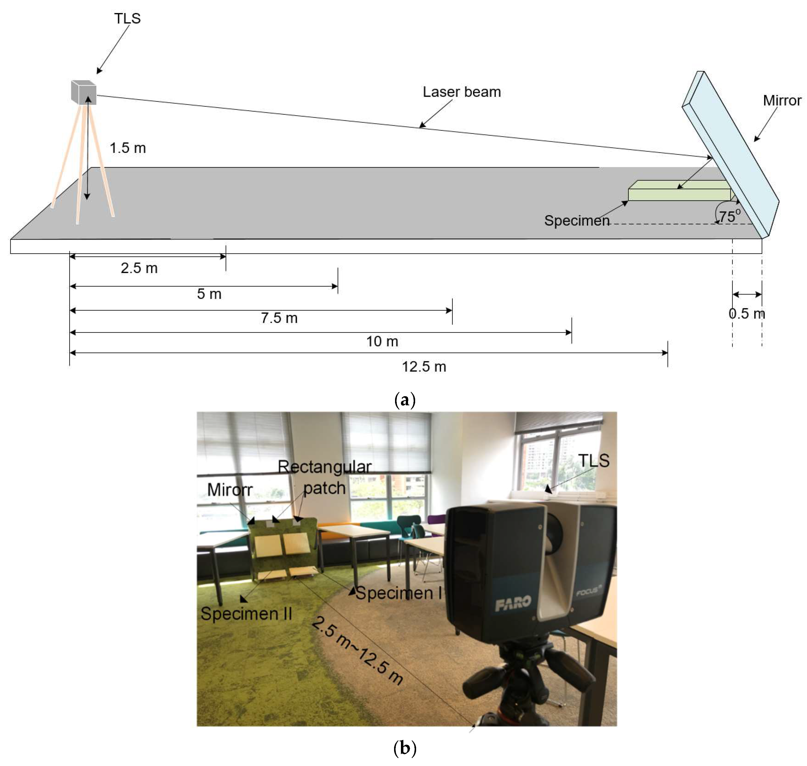
4.1. Experimental Setup
4.2. Data Processing
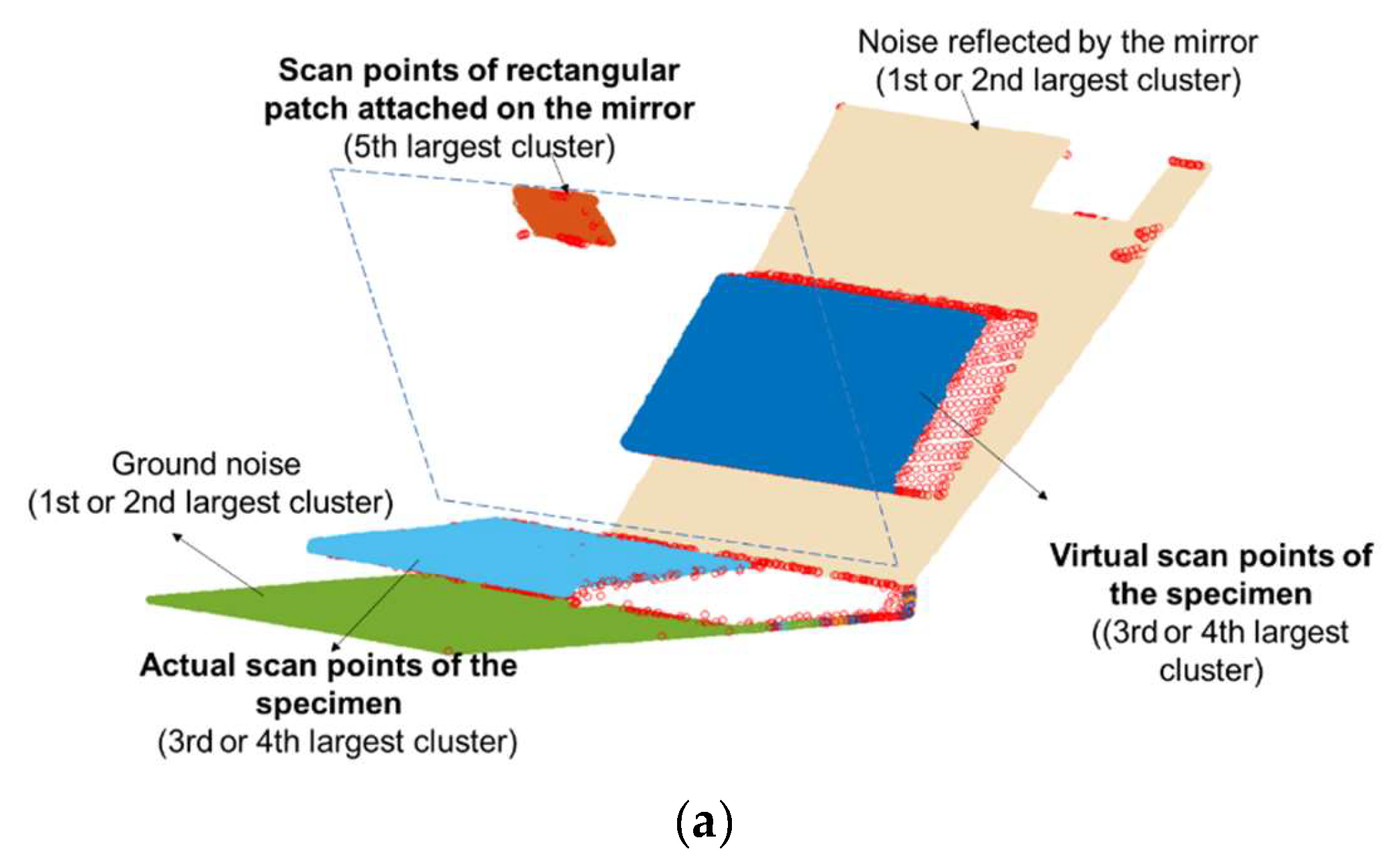
4.2.1. Data Preprocessing
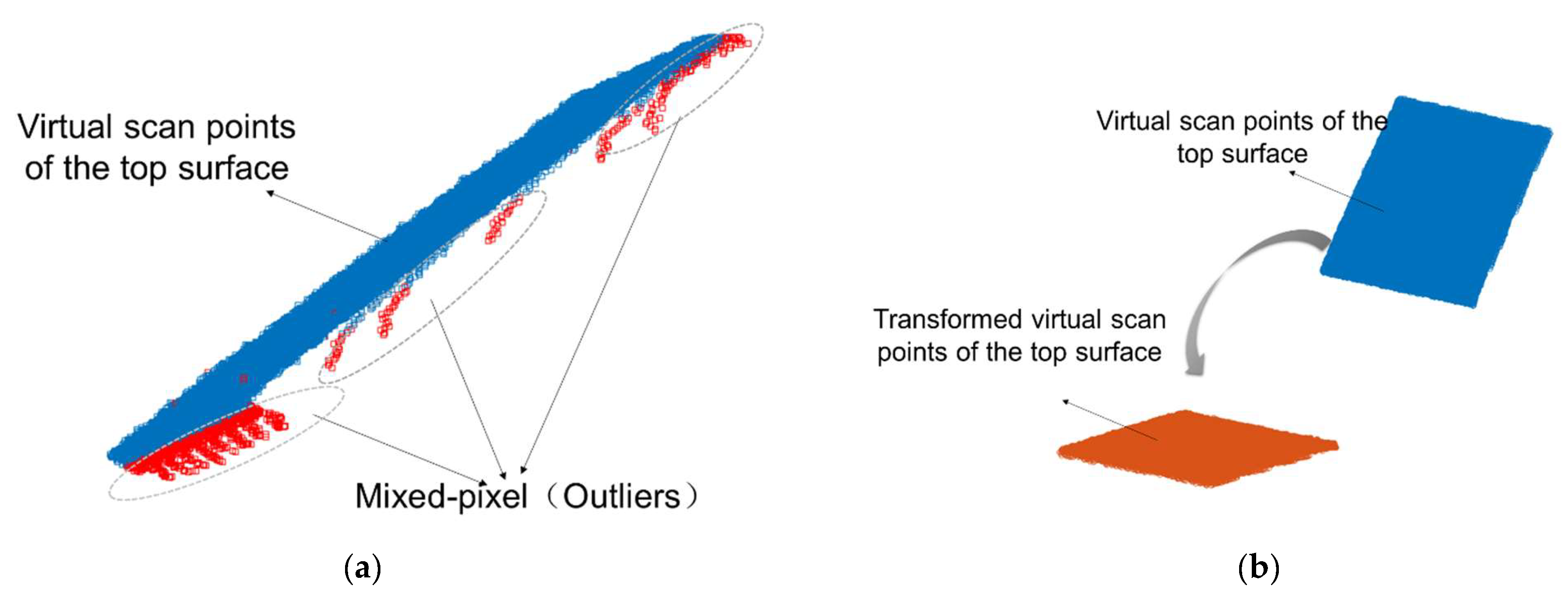
4.2.2. Virtual Scan Points Transformation
4.2.3. Surface Flatness Calculation
5. Results
6. Discussion
6.1. Performance Comparison with Combined Scan Points
6.2. Mirror Location and Mirror Size for Performing Surface Flatness Inspection
7. Conclusions
Author Contributions
Funding
Conflicts of Interest
References
- British Standards Institution (BSI). BS 8204-Screeds, Bases and In Situ Flooring; BSI: London, UK, 2009. [Google Scholar]
- American Concrete Institute (ACI). ACI 117-06-Specifications for Tolerances for Concrete Construction and Materials and Commentary; ACI: Farmington Hills, MI, USA, 2006. [Google Scholar]
- Hieber, D.G.; Wacker, J.M.; Eberhard, M.O.; Stanton, J.F. State-of-the-Art Report on Precast Concrete Systems for Rapid Construction of Bridges. Washington State Transportation Center. (No. WA-RD 594.1); 2005. Available online: https://rosap.ntl.bts.gov. (accessed on 20 August 2020).
- American Concrete Institute (ACI). ACI 302.1R-96 -Guide for Concrete Floor and Slab Construction; ACI: Farmington Hills, MI, USA, 1997. [Google Scholar]
- Shih, N.; Wang, P. Using Point Cloud to Inspect the Construction Quality of Wall Finish. In Proceedings of the 22nd eCAADe Conference, Copenhagen, Denmark, 15–18 September 2004; pp. 573–578. Available online: http://cumincad.scix.net/data/works/att. (accessed on 1 August 2020).
- Li, D.; Liu, J.; Feng, L.; Zhou, Y.; Liu, P.; Chen, Y.F. Terrestrial laser scanning assisted flatness quality assessment for two different types of concrete surfaces. Measurement 2020, 154, 107436. [Google Scholar] [CrossRef]
- American Society for Testing (ASTM). ASTM E 1155-96-Standard Test Method for Determining FF Floor Flatness and FL Floor Levelness Numbers; ASTM: West Conshohocken, PA, USA, 2008. [Google Scholar]
- Bosché, F.; Biotteau, B. Terrestrial laser scanning and continuous wavelet transform for controlling surface flatness in construction—A first investigation. Adv. Eng. Inform. 2015, 29, 591–601. [Google Scholar] [CrossRef]
- Kim, M.-K.; Wang, Q.; Li, H. Non-contact sensing based geometric quality assessment of buildings and civil structures: A review. Autom. Constr. 2019, 100, 163–179. [Google Scholar] [CrossRef]
- Kim, M.-K.; Thedja, J.P.P.; Wang, Q. Automated dimensional quality assessment for formwork and rebar of reinforced concrete components using 3D point cloud data. Autom. Constr. 2020, 112, 103077. [Google Scholar] [CrossRef]
- Kim, M.-K.; Wang, Q.; Yoon, S.; Sohn, H. A mirror-aided laser scanning system for geometric quality inspection of side surfaces of precast concrete elements. Measurement 2019, 141, 420–428. [Google Scholar] [CrossRef]
- Wang, Q.; Tan, Y.; Mei, Z. Computational Methods of Acquisition and Processing of 3D Point Cloud Data for Construction Applications. Arch. Comput. Methods Eng. 2019, 27, 479–499. [Google Scholar] [CrossRef]
- Kim, M.-K.; Sohn, H.; Chang, C.C. Localization and Quantification of Concrete Spalling Defects Using Terrestrial Laser Scanning. J. Comput. Civ. Eng. 2015, 29, 04014086. [Google Scholar] [CrossRef]
- Tang, P.; Huber, D.; Akinci, B. Characterization of Laser Scanners and Algorithms for Detecting Flatness Defects on Concrete Surfaces. J. Comput. Civ. Eng. 2011, 25, 31–42. [Google Scholar] [CrossRef]
- Yoo, M.; Ham, N. Productivity Analysis of Documentation Based on 3D Model in Plant Facility Construction Project. Appl. Sci. 2020, 10, 1126. [Google Scholar] [CrossRef]
- Ham, N.; Lee, S.H. Empirical Study on Structural Safety Diagnosis of Large-Scale Civil Infrastructure Using Laser Scanning and BIM. Sustainability 2018, 10, 4024. [Google Scholar] [CrossRef]
- Erdélyi, J.; Kopáčik, A.; Kyrinovič, P. Spatial Data Analysis for Deformation Monitoring of Bridge Structures. Appl. Sci. 2020, 10, 8731. [Google Scholar] [CrossRef]
- FARO. Faro® Laser Scanner Focus. Available online: https://www.faro.com/ensg/products/construction-bim/faro-laser-scanner-focus (accessed on 20 August 2020).
- Wang, Q.; Kim, M.-K.; Sohn, H.; Cheng, J.C. Surface flatness and distortion inspection of precast concrete elements using laser scanning technology. Smart Struct. Syst. 2016, 18, 601–623. [Google Scholar] [CrossRef]
- Bosché, F.; Guenet, E. Automating surface flatness control using terrestrial laser scanning and building information models. Autom. Constr. 2014, 44, 212–226. [Google Scholar] [CrossRef]
- Puri, N.; Valero, E.; Turkan, Y.; Bosché, F. Assessment of compliance of dimensional tolerances in concrete slabs using TLS data and the 2D continuous wavelet transform. Autom. Constr. 2018, 94, 62–72. [Google Scholar] [CrossRef]
- C. Standard. GB50204-2015-Code for Acceptance of Construction Quality of Concrete Structures; C. Standard: Beijing, China, 2015. [Google Scholar]
- Sinha, S.; Routh, P.S.; Anno, P.D.; Castagna, J.P. Spectral decomposition of seismic data with continuous-wavelet transform. Geophysics 2005, 70, P19–P25. [Google Scholar] [CrossRef]
- ASTM International. ASTM E 1486 -Standard Test Method for Determining Floor Tolerance Using Waviness, Wheel Path, and Levelness Criteria; ASTM: West Conshohocken, PA, USA, 2010. [Google Scholar]
- ZRAPID. ZRAPID SLA 3D Printer. Available online: http://www.zero-tek.com/en/sla880.html (accessed on 1 August 2020).
- Ram, A.; Jalal, S.; Jalal, A.S.; Kumar, M. A Density Based Algorithm for Discovering Density Varied Clusters in Large Spatial Databases. Int. J. Comput. Appl. 2010, 3, 1–4. [Google Scholar] [CrossRef]
- Tang, P.; Akinci, B.; Huber, D. Quantification of edge loss of laser scanned data at spatial discontinuities. Autom. Constr. 2009, 18, 1070–1083. [Google Scholar] [CrossRef]
- Fischler, M.A.; Bolles, R.C. Random Sample Consensus: A Paradigm for Model Fitting with Applications to Image Analysis and Automated Cartography. Read. Comput. Vis. 1987, 24, 726–740. [Google Scholar] [CrossRef]
- Pratt, V. Direct least-squares fitting of algebraic surfaces. ACM SIGGRAPH Comput. Graph. 1987, 21, 145–152. [Google Scholar] [CrossRef]
- He, Y.; Liang, B.; Yang, J.; Li, S.; He, J. An Iterative Closest Points Algorithm for Registration of 3D Laser Scanner Point Clouds with Geometric Features. Sensors 2017, 17, 1862. [Google Scholar] [CrossRef] [PubMed]
- Li, F.; Kim, M.; Li, H. Registration-free 3D point cloud data acquisition technique for as-is BIM generation using rotating flat mirrors. In Proceeding of the 8th International Conference on Construction Engineering and Project Management, Hong Kong, China, 7–8 December 2020; pp. 3–12. Available online: http://www.iccepm2019.com/wp-content/uploads/2020/12/Proceedings-of-ICCEPM-2020.pdf (accessed on 12 December 2020).


| Surface Flatness Classification | Deviations of Elevation | FF Numbers | Thresholds Used for Validation (20% of the Deviations of Elevation) |
|---|---|---|---|
| Conventional | 13 mm | 20 | 2.6 mm |
| Moderately flat | 10 mm | 25 | 2.0 mm |
| Flat | 6 mm | 35 | 1.2 mm |
| Very flat | 5 mm | 45 | 1.0 mm |
| Super flat | 3 mm | 60 | 0.6 mm |
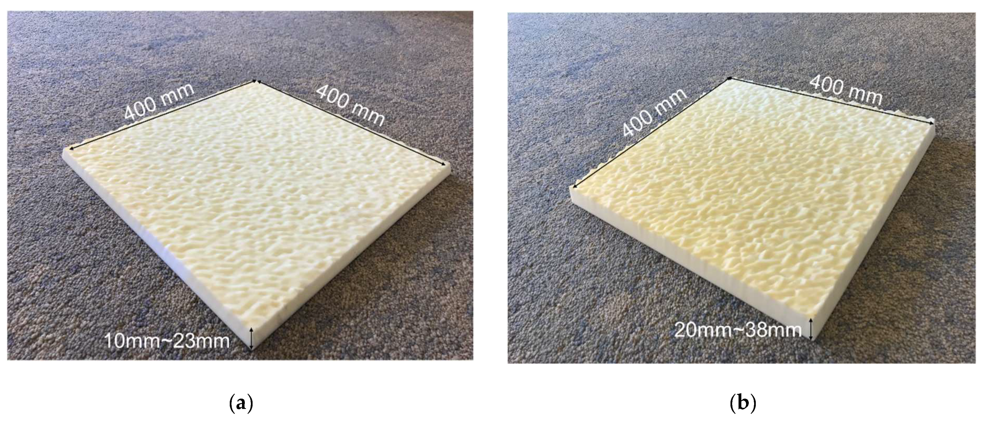
| Items | Size (Length × Width × Height) | FF Numbers |
|---|---|---|
| Specimen I | 400 mm × 400 mm × 10–23 mm | 10.28 |
| Specimen II | 400 mm × 400 mm × 20–38 mm | 21.23 |
| Object | Scanning Distance (Incident Angle) | Estimation Error of FF Numbers Specimen I in Percentage (Data Density: pts/cm2) | Estimation Error of FF Numbers Specimen II in Percentage (Data Density: pts/cm2) | ||
|---|---|---|---|---|---|
| Angular Resolution | Angular Resolution | ||||
| 0.036° | 0.072° | 0.036° | 0.072° | ||
| Virtual scan points | 2.5 m (51°) | 9.5% (87.7) | 13.8% (21.9) | 3.9% (87.2) | 8.4% (21.9) |
| 5 m (43°) | 9.6% (27.0) | 11.1% (6.7) | 4.0% (27.1) | 19.1% (6.7) | |
| 7.5 m (40°) | 18.6% (12.7) | 37.1% (3.2) | 8.9% (12.9) | 11.7% (3.2) | |
| 10 m (38°) | 15.1% (7.3) | 49.0% (1.8) | 19.8% (7.3) | 23.3% (1.8) | |
| 12.5 m (37°) | 31.1% (4.9) | 49.1% (1.2) | 20.9% (4.8) | 37.0% (1.2) | |
| Actual scan points | 2.5 m (70°) | 19.9% (67.3) | 36.1% (16.6) | 4.4% (64.9) | 27.0% (16.6) |
| 5 m (79°) | 82.5% (10.6) | 83.1% (2.7) | 19.8% (10.6) | 19.5% (2.5) | |
| 7.5 m (82°) | 161.4% (3.6) | 140.5% (0.9) | 58.7% (3.3) | 88.4% (0.8) | |
| 10 m (84°) | 211.1% (1.5) | 278.8% (0.4) | 107.3% (1.4) | 143.0% (0.3) | |
| 12.5 m (86°) | 210.3% (0.70) | −0.20 | 155.6% (0.60) | −0.20 | |
| Object | FF Numbers Estimation Error of Specimen I (mm) | FF Numbers Estimation Error of Specimen II (mm) | ||||
|---|---|---|---|---|---|---|
| Angular Resolution | Angular Resolution | |||||
| 0.036° | 0.072° | Ave. | 0.036° | 0.072° | Ave. | |
| Estimation error in percentage | 10.7% | 27.6% | 14.3% | 10.4% | 11.8% | 11.1% |
| Object | Data Density of Specimen I (pts/cm2) | Data Density of Specimen II (pts/cm2) | ||||
|---|---|---|---|---|---|---|
| Angular Resolution | Angular Resolution | |||||
| 0.036° | 0.072° | Ave. | 0.036° | 0.072° | Ave. | |
| Combined scan points | 54.3 | 13.6 | 34.0 | 53.7 | 13.5 | 33.6 |
| Virtual scan points | 33.6 | 8.4 | 21.0 | 33.6 | 8.4 | 21.0 |
| Actual scan points | 20.7 | 5.2 | 13.0 | 20.1 | 5.1 | 12.6 |
| Items | Determined Results | |
|---|---|---|
| Mirror Position I | Mirror Position II | |
| Mirror rotation angle | 68° | 55° |
| Scan coverage | 5.0 m–7.8 m | 7.8 m–10.0 m |
| Scan density | 8.2 pts/cm2 | 11.1 pts/cm2 |
Publisher’s Note: MDPI stays neutral with regard to jurisdictional claims in published maps and institutional affiliations. |
© 2021 by the authors. Licensee MDPI, Basel, Switzerland. This article is an open access article distributed under the terms and conditions of the Creative Commons Attribution (CC BY) license (http://creativecommons.org/licenses/by/4.0/).
Share and Cite
Li, F.; Li, H.; Kim, M.-K.; Lo, K.-C. Laser Scanning Based Surface Flatness Measurement Using Flat Mirrors for Enhancing Scan Coverage Range. Remote Sens. 2021, 13, 714. https://doi.org/10.3390/rs13040714
Li F, Li H, Kim M-K, Lo K-C. Laser Scanning Based Surface Flatness Measurement Using Flat Mirrors for Enhancing Scan Coverage Range. Remote Sensing. 2021; 13(4):714. https://doi.org/10.3390/rs13040714
Chicago/Turabian StyleLi, Fangxin, Heng Li, Min-Koo Kim, and King-Chi Lo. 2021. "Laser Scanning Based Surface Flatness Measurement Using Flat Mirrors for Enhancing Scan Coverage Range" Remote Sensing 13, no. 4: 714. https://doi.org/10.3390/rs13040714
APA StyleLi, F., Li, H., Kim, M.-K., & Lo, K.-C. (2021). Laser Scanning Based Surface Flatness Measurement Using Flat Mirrors for Enhancing Scan Coverage Range. Remote Sensing, 13(4), 714. https://doi.org/10.3390/rs13040714