1. Introduction
Ice caps, ice plugs, or ice dams are often formed in high latitude rivers in winter, which could change the hydraulic, thermal, and geometric boundary conditions of water flow and form a unique ice phenomenon in winter [
1]. Ice plugs or ice dams, i.e., drift ice in the river channel blocking the cross section of water flow, may cause water level rise, inundate farmland houses, damage the coastal hydraulic structures, cause shipping interruption, or cause hydraulic power loss [
2,
3]. Therefore, river ice monitoring is necessary in preparing for potential hazards. Accurate fine-grained ice semantic segmentation is a key technology in the study of river ice monitoring, which can provide more information for ice situation analysis, change trend prediction, and so on.
Many efforts have been spent on studying river ice segmentation based on imaging monitoring. In terms of monitoring, there are typically three kinds, including satellite-based monitoring [
4,
5,
6,
7], shore-based terrestrial monitoring [
8,
9], and UAV (unmanned aerial vehicle)-based aerial monitoring [
10,
11,
12]. The advantage of satellite-based monitoring is that its observation range is very large and it is not limited by national boundaries and geographical conditions. While, it is often hard or costly to realize real-time observation. The revisit period of general satellites like Landsat is often several days. Some satellites with short revisit periods are often expensive or have coarse resolution. Shore-based terrestrial monitoring can observe river ice at any time. But, installing surveillance equipment on the shore is often limited by geographical conditions, especially in mountainous regions. UAV-based aerial monitoring has the advantages of having a wide monitoring range, a fast response speed, and is uneasily disturbed by terrain. It has served as an important supplementary way to monitor river ice. Therefore, this paper focuses on the monitoring of river ice using UAV images.
In terms of ice segmentation methods, they are divided into three categories: Traditional threshold methods, traditional machine learning-based methods, and neural network-based methods. Note that, here we also consider the methods of sea ice segmentation, since they are similar to river ice segmentation to a certain extent.
Traditional threshold methods. The threshold-based segmentation methods use the difference in gray scale of different objects to be extracted from the image, and divide the pixels into several categories by setting appropriate threshold values to achieve the segmentation of different objects. Engram et al. [
6] utilized a threshold approach to distinguish floating ice and bedfast ice using SAR images across Arctic Alaska. Beaton et al. [
7] presented a river coverage segmentation method, in which a threshold technique was adopted to reduce the effectiveness of cloud obstruction and maximize river coverage.
Traditional machine learning-based methods. With the development of machine learning, many methods have been utilized to segment an ice region from images. They can be summarized into two categories, unsupervised and supervised methods. On the part of unsupervised methods, Ren et al. [
13] presented a multi-stage method using k-means clustering for sea ice SAR image segmentation. Dang et al. [
14] presented two methods for SAR sea ice image segmentation: The k-means clustering method and threshold-based segmentation method. The result showed that the k-means clustering method outperformed the threshold-based segmentation method. The former can gain a clear segmentation boundary and complete segmentation region. Chu and Lindenschmidt [
4] classified the river covers into four categories, including smooth rubble ice, intact sheet ice, rough rubble ice, and open water, based on fuzzy k-means clustering with Moderate Resolution Imaging Spectroradiometer (MODIS) and RADARSAT-2 images. On the part of supervised methods, Zhang et al. [
15] presented a CART decision tree method to retrieve sea ice from MODIS images in the Bohai Sea. Romanov [
5] adopted decision tree to detect ice using AVHRR images.
Deep neural network-based methods. In recent years, we have witnessed important advances in image semantic segmentation based on deep neural networks. A new generation of algorithms based on FCN [
16] keeps improving state-of-the-art performance on different benchmarks. Singh et al. [
11] adopted several deep neural network-based semantic segmentation models to segment river ice images into anchor ice, frazil ice, and water, and achieved great outcomes. These models are mainly UNet [
17], SegNet [
18], and DeepLab [
19]. In 2020, we [
12] also designed a semantic segmentation deep convolution neural network, named ICENET, for river ice semantic segmentation. It revealed that applying deep convolutional neural networks into ice detection and fine-grained ice segmentation is promising.
In conclusion, the traditional threshold method directly utilizes the gray-scale differential characteristics of the images and has the advantages of simple calculation and high efficiency. However, an appropriate threshold is hard to be determined and is sensitive to many factors such as noise and brightness. Therefore, this kind of method usually has a poor generalization ability. The traditional machine learning-based methods can achieve good results for tasks in simple scenes, but with images of complex scenes, they are still relatively simple and require manual intervention, which cannot guarantee the segmentation effect. With the popularity of deep learning, semantic segmentation has made great progress. Convolutional neural network-based semantic segmentation methods far exceed traditional methods, under its strong nonlinear fitting ability and learning ability. Hence, the deep neural network-based method is adopted in this paper.
In this paper, we study fine-grained river ice segmentation based on the deep neural network technique. This study is different from the methods mentioned above. It distinguishes shore ice, drift ice, water, and bank, which has an important application significant in river ice monitoring. Therefore, to study it, a UAV image dataset was built. By analysis, this fine-grained river ice segmentation has these characteristics: (1) The scale of river ice varies greatly, ranging from several pixels to thousands of pixels; (2) the appearances of river ice are diverse, even for the same kind; and (3) sometimes, drift ice and shore ice look similar, since they could become each other in some conditions. There characteristics will be analyzed in
Section 2.2. Aiming towards these characteristics, we designed a novel semantic segmentation network structure, which effectively exploits the multilevel features fusion, dual attention module, and new up-sampling strategy to generate high-resolution predictions. Our main contributions are as follows:
A UAV image dataset named NWPU_YRCC2 was built for fine-grained river ice semantic segmentation. All UAV images were collected in the Ningxia–Inner Mongolia reach of the Yellow River, since the ice phenomenon in this reach is very typical and diverse. The dataset consists of 1525 precisely labeled images covering typical river ice images with different characteristics;
A novel network is proposed for fine-grained river ice segmentation, named ICENETv2. In this network, multiscale low-resolution semantic features and high-revolution finer features are effectively fused to generate different scale predictions, since the scale of river ice changes greatly even in the same image. Additionally, we adopt a dual attention module to highlight distinguishable features and use a learnable up-sampling strategy to improve the details of the segmentation and increase the semantic segmentation accuracy of fine-grained river ice;
Compared with DeepLabV3 [
20], PSPNet [
21], RefineNet [
22], and BiseNet [
23], our ICENETv2 has the state-of-the-art performance on the NWPU_YRCC2 dataset. Besides, our ICENETv2 is applied to solve a practical problem, i.e., calculating drift ice cover density, which is one of the most intuitive information for predicting the freeze-up date of a river. By using the predicted fine-grained river ice semantic segmentation map, the drift ice cover density error is only 5.6%. The results show that its performance meets the actual application demand.
3. Proposed Method
We propose a novel semantic segmentation network, named ICENETv2, to deal with the challenges of fine-grained river ice segmentation. ICENETv2 is developed based on our previous ICENET and it differs from ICENET in four main respects. Aiming to extract more multi-scale high-level semantic information, the ratios of the feature maps of Res1, Res2, Res3, and Res4 to the input image are changed from (1/8, 1/16, 1/16, 1/16) to (1/4, 1/8, 1/16, 1/32), respectively. Both position attention and channel attention are adopted to highlight the distinguishable semantic features between drift ice and shore ice. A learnable up-sampling strategy is used to further reconstruct the finer information, since the appearance of drift ice is diverse and sometimes its scale is prone to be small. Finally, a joint loss function is utilized to sufficiently train the network.
In this section, firstly, the network architecture of our ICENETv2 is illustrated, as shown in
Figure 4. Secondly, the four principle sub-modules of ICENETv2, namely attention module, fusion module, sub-pixel upsample module [
28], and the loss function are presented in
Section 3.2,
Section 3.3,
Section 3.4,
Section 3.5 respectively.
3.1. Network Architecture
In fine-grained river ice semantic segmentation, the scales of the drift ice and shore ice vary diversely, ranging from several pixels to hundreds of pixels, even thousands of pixels. The effective fusion of multiscale features can significantly enhance the segmentation precision of multiscale targets. Therefore, inspired by BiseNet, the proposed ICENETv2 also adopts a two-branch architecture, as shown in
Figure 4. The deep branch aims to extract high-level semantic context features, in which a parallel dual attention mechanism combining channel attentive features and positional attentive features is adopted to extract more comprehensive and sufficient semantic features. The shallow branch extracts low-level features that can encode high-resolution finer spatial details. Finally, deep features and shallow features are sufficiently fused to generate prediction. Besides, instead to the commonly used bilinear interpolation, a learnable up-sampling strategy, i.e., sub-pixel method [
28], is utilized to further refine the segmentation detail.
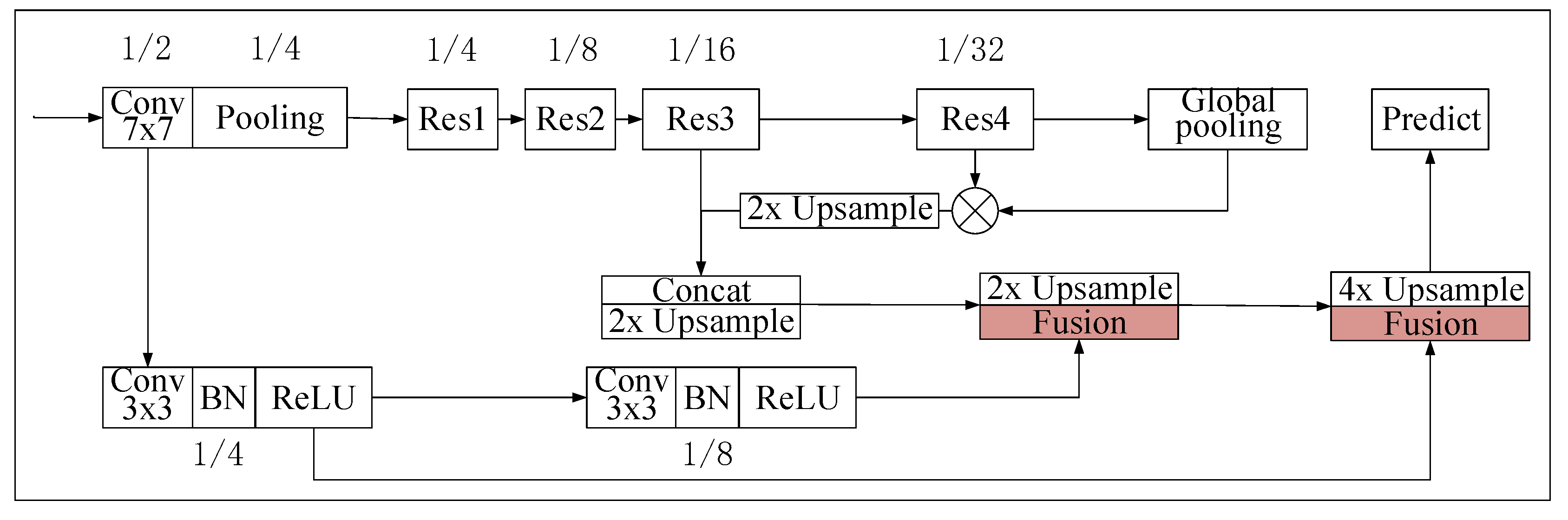
To be specific, the input image is fed into a convolution block, of which stride is 2 and kernel size is 7. Then, in order to acquire semantic context features and detailed finer features, the output features are respectively input into two branches. The deep branch is based on ResNet-101 and consists of four residual blocks, namely Res1, Res2, Res3, and Res4. The four residual blocks are original residual blocks in ResNet-101. The stride of Res1 is 1 and that of the other three blocks is 2. Res3 and Res4 are separately followed by a parallel dual attention module, in which channel attention and positional attention are parallel imposed on the output of the residual block, then the two attentive features are combined by element-wise sum as the output. A global average pooling is performed on the output of Res4 to produce a global contextual vector. Then, the output features of dual attention module after Res4 are weighted by the global contextual vector and the weighted output is up-sampled twice by the sub-pixel method [
28]. Finally, we concatenate the weighted features after up-sampling and output features of the dual attention module after Res3, then up-sample them twofold by sub-pixel to generate multiscale semantic features as the output of the deep branch.
The shallow branch only contains two convolution blocks, of which stride is 2 and kernel size is 3. Therefore, there are two outputs corresponding to the two convolution blocks. The size of the two output feature maps is one-quarter and one-eighth of the input image size, respectively. Since there are many small drift ice blocks in the problem of fine-grained river ice semantic segmentation, the shallow branch is designed to gain two different scales of high-resolution spatial information.
Finally, the fusion module shown in
Figure 5 is adopted to integrate the two branch outputs to generate ultimate prediction. Firstly, the output feature maps of the deep branch and shallow one-eighth resolution output feature maps are fused and up-sampled twice by sub-pixel. Then, the former fusion result and the one-quarter resolution output feature maps of the shallow branch are fused again and 4X up-sampled by the bilinear interpolation, to achieve the final semantic segmentation prediction.
3.2. Attention Model
It is a very common ice phenomenon that drift ice blocks may crash or rub with shore ice, some of which stop at the edge of the shore ice and freeze up to become a new part of shore ice. In this situation, it is not easy to distinguish drift ice and shore ice. Therefore, context information with spatial and semantic distinguishability is required. Inspired by DANet [
29], we adopt a dual-attention module in the deep branch of our model, which contains a channel attention and a positional attention. The channel attention model can integrate the relevant features of all channels, so as to generate global association between channels and obtain stronger specific semantic response ability. The local correlation of spatial information can be learned by positional attention model, and the correlation between features of any position can be used to enhance the expression of their respective features. Then, the fusion of the above two kinds of enhanced attentive features will make the extracted features more effective to distinguish different kinds of objects.
Figure 6a shows the details of the channel attention module. Firstly, four operations, i.e., a global average pooling, a 1 × 1 convolution, a batch normalization, and a sigmoid function, are successively performed on the input feature map
to produce an attentive vector. Then, the attentive vector is used to weigh the input feature map, and the result is element-wise added with the input feature map to generate channel-wise attentive feature
.
The structure of the position attention module is presented in
Figure 6b. Given the input feature map
,
is input into three
convolution blocks to produce three feature maps
,
, and
, where
. Meanwhile,
,
, and
are reshaped to
, where
. Subsequently, we multiply the transpose of
by
, and utilize a softmax operation to produce a positional attention map
. Then, we multiply the transpose of
by
and reshape the result to
. Lastly, the feature
is obtained by element-wise addition between the reshaped result and the feature map
.
3.3. Fusion Module
The outputs of the deep branch and shallow branch represent semantic context information and detailed information, respectively. Both of them can greatly help to process accurate segmentation. To combine these features of two different levels and play to their strengths, an effective feature fusion strategy is required. The feature fusion module in [
23] is adopted, as shown in
Figure 5. Firstly, we concatenate the output features of the deep branch and the shallow branch, then a 1 × 1 convolution, a batch normalization, and a ReLu function is performed on the concatenated feature maps successively. Finally, a sub-module shown in the yellow dotted box, which looks alike to the channel attention module, is calculated to produce the fusion result. The only differences between the sub-module and channel attention module are that batch normalization in the channel attention module is replaced by a ReLu function and a 1 × 1 convolution.
3.4. Sub-Pixel Up-Sampling Module
Sub-pixel up-sampling derives from super resolution research [
28] and has been used in semantic segmentation and other tasks. As shown in
Figure 7, assuming that the input is a low-resolution image or feature map, the sub-pixel up-sampling is to extract the features from the input and finally fuse the extracted features to generate high-resolution (HR) images. Three convolution layers are adopted in detail. After that, the feature maps of channel number
are obtained, in which
r is the magnification factor. Then, through the sub-pixel convolution layer,
channels of each pixel are transformed to a sub-pixel block with size
in the HR image. Finally, the feature map of
is reshaped to a HR map of
. To upsample feature maps with more than one channel, sub-pixel up-sampling strategy is applied to each channel.
3.5. Loss Function
In our model, auxiliary losses are adopted to supervise the training of the proposed network. The main loss is used to supervise the final prediction of the whole ICENETv2. Three particular auxiliary losses are utilized to supervise the outputs of two dual attention modules respectively after Res3 and Res4 and the output of the first fusion model. Categorical cross-entropy loss is adopted as the loss function for these four losses, as shown in Equation (
1). Meanwhile, parameter
is adopted to balance the weight of the main loss and three auxiliary losses, as presented in Equation (
2). The three auxiliary losses share a weight
, since the orders of magnitude of them are the same and they are all utilized to supervise intermediate feature maps without significant difference in importance. We conducted an ablation experiment on three auxiliary losses and an experiment to find a reasonable parameter
. The details refer to
Section 4.3. Finally,
is set to 1 in our subsequent experiments. The joint loss allows the optimizer to optimize the model more conveniently.
where n indicates n classes,
is the truth label and
is the Softmax probability for the
ith class.
where
denotes the hyper-parameter of controlling the relative importance of the three auxiliary loss terms.
is the main loss function.
and
are used to supervise the outputs of two dual attention modules after Res3 or Res4, respectively.
is used to optimize the output of the first fusion.
,
,
, and
are calculated by Equation (
1).
is the joint loss function.
4. Experiments
In this section, firstly, the implementation details of the experiments are described. Secondly, the ablation experimental results performed on NWPU_YRCC2 are illustrated and analyzed. Thirdly, our ICENETv2 model is compared with some state-of-the-art methods. Finally, our model is utilized to solve an actual application, calculating the drift ice cover density.
4.1. Implementation Details
Our models are implemented based on Pytorch. In the training procedure, mini-batch stochastic gradient descent [
30] is adopted, the momentum is initially set to 0.9, and decays by weight
with a batch size of 4. The training time is set to 200 epochs. The overall training time for 200 epochs takes about 30 h on two NVIDIA GeForce GTX 2080Ti cards and the training time per epoch of our model is about 9 minutes. After about 120 trained epochs, our model converges. Our NWPU_YRCC2 dataset contains 1525 annotated images. In the experiments, it is divided into a training set, validation set. and test set at a ratio of 6:2:2, then the segmentation results were colored for better visualization. The NWPU_YRCC dataset contains a total of 814 annotated images, including 570 images for training, 82 images for verification, and 244 images for testing. Note that the test set includes the verification set.
4.2. Evaluation
Pixel accuracy and mean intersection over union are usually adopted to measure the accuracy of semantic segmentation. Therefore, we used these two indicators to calculate and compare the performances of different methods. Assume that there are totally n + 1 categories (from 0 to n) and class 0 indicates a void class or background. is the amount of pixels that belong to class i but were predicted to be class j. is the amount of pixels of class i and were predicted to be class i. When and class i is regarded as positive, and is the number of false positives and false negatives, respectively. PA (pixel accuracy) and MIoU (mean intersection over the union) can be described as follows.
Pixel accuracy (PA). PA, described in Equations (
3), is the ratio of the number of correctly classified pixels to the overall amount of pixels:
Mean intersection over the union (MIoU). IoU is the ratio of the intersection area of the predicted segmentation with the ground truth to the union area of them for one particular class. MIoU is often adopted to measure the accuracy for the segmentation of more than one class. It denotes the average value of the IoUs of all classes. The specific description is shown in Equation (
4):
4.3. Ablation Study
To verify the effect and contribution of three auxiliary losses, we conduct an ablation experiment on them as shown in
Table 2. The network is trained and optimized by one main loss function and two selected auxiliary loss functions at a time. The results show that these three auxiliary losses all contribute to the final semantic segmentation and there is no significant difference in importance among them. These three auxiliary losses share a weight
. To find a reasonable parameter
, we also conducted an experiment shown in
Table 3. It shows that when
, the method performs best. Therefore, we chose
in our subsequent experiments.
To verify the effects of the proposed model and their three principle sub-modules, we conducted another ablation experiment successively adding the channel attention, the position attention, sub-pixel up-sampling, and auxiliary loss to the baseline model.
Table 4 shows the results of these ablation experiments. The first row shows the results of the baseline model, which is depicted in
Figure 8. Compared with ICENETv2, the baseline does not contain the dual attention model and sub-pixel up-sampling model, and its loss only considers the main loss. In
Table 4, ‘CAM’ and ‘PAM’ respectively denotes adding channel attention and position attention after the block Res3 and Res4. ‘CAM + PAM’ means adding both attention modules after the block Res3 and Res4. The notation ’Sub-pixel’ means that part of up-sampling operations are sub-pixel up-sampling shown in
Figure 4. The notation ‘Au_loss’ means that three auxiliary losses are also considered in the loss function.
The experimental results show that MIoU has increased by 2.674% by adding only the position attention module in the baseline model and 3.760% by adding only the channel attention module. When the two attention modules are adopted simultaneously in the baseline model, the MIoU is increased by 4.249%. On this basis, sub-pixel and Au_loss modules are added respectively, and MIoU is improved by 2.449% and 1.922% respectively. When all the sub-modules of the ablation experiment are added to the baseline module, the MIoU achieves 83.435%.
Moreover,
Figure 9 shows some visualization results to demonstrate the effectiveness of the two attention modules. By adding the position attention module or channel attention module to the baseline model, the fine-grained semantic segmentation of drift ice is more accurate and some details and object boundaries are clearer.
4.4. Comparison with the State-of-the-Art
The methods DeepLabV3 [
20], DenseASPP [
31], PSPNet [
21], RefineNet [
22], and BiseNet [
23] have achieved excellent performance on public datasets. They are the representive semantic segmentation methods of the state-of-the-art. Therefore, we compare the proposed ICENETv2 with them on NWPU_YRCC2 and NWPU_YRCC. The comparison results are presented in
Table 5. They demonstrate that the ICENETv2 has a significant improvement in terms of MIoU on NWPU_YRCC2, meanwhile the single-class in terms of IoU for the drift ice is also the highest.
Figure 10 presents some visualization comparison results. We can see that the results of the ICENETv2 have a better segmentation and recognition accuracy of small-scale targets. The experimental results also show that the performance of ICENETv2 on NWPU_YRCC is significantly higher than that of other methods and slightly higher than that of ICENET. This can further verify the effectiveness of ICENETv2 on fine-grained segmentation.
4.5. Application on the Calculation of Drift Ice Cover Density
Drift ice cover density is one of the most important factors in predicting the freeze-up date of river and can provide more information for ice situation analysis. Now manual visual measurement is still adopted to calculate the drift ice cover density in many hydrological stations. This measurement way is greatly affected by human experience, and is usually prone to error. Based on the predicted fine-grained river ice semantic segmentation map, the drift ice cover density can be calculated automatically, as shown in Equation (
5). The Drift_Ice_Num and River_Water_Num in Equation (
5) represents the pixel number of water and drift ice respectively, in the predicted fine-grained river ice semantic segmentation map:
To accurately calculate the drift ice cover density, the UAV lens should be perpendicular to the river surface. At the same time, the bank on both side of the river should be included in the shooting process, so that the bank can be viewed. We selected five typical scenes to verify our calculation, as shown in
Figure 11. The error between the drift ice cover density calculated by the predicted fine-grained river ice semantic segmentation map and that by the label is only 5.6%. This demonstrates that our method is accurate enough to meet actual application requirements.
4.6. Discussion
From the ablation experiments, it can be seen that ICENETv2 is 7.224% higher on MIoU than the baseline model and each sub-module has a certain contribution. The visualization results shown in
Figure 8 also exhibit the improvement effect on the segmentation detail of the attention module and the sub-pixel up-sampling. By adding these sub-modules mentioned above to the baseline model, our ICENETv2 achieved the highest IoU in the drift ice category, reaching 81.127% IoU, indicating that our model is suitable for fine-grained segmentation.
The proposed ICENETv2 is compared on our NWPU_YRCC2 dataset with the state-of-the-art methods, including DeepLabV3 [
20], DenseASPP [
31], PSPNet [
21], RefineNet [
22], and BiseNet [
23]. The experimental results indicate that the proposed method achieves significant improvements over the state-of-the-art methods in terms of mean IoU. Although our method is inspired by BiseNet to some extent, it is carefully designed to adapt the characteristics of fine-grained segmentation. It adopts a new fusion structure to effectively fuse high-level semantic information and low-level finer information, and utilizes dual-attention [
29] to highlight the distinguishable semantic features between drift ice and shore ice. A learnable up-sampling strategy [
28] is used to further reconstruct the finer information, since the appearance of drift ice is diverse and sometimes its scale is prone to be small. In addition it has a joint loss function with three auxiliary losses to sufficiently train the network. These three parts are different from BiseNet. The experimental results on NWPU_YRCC2 can demonstrate our design is effective to the problem of fine-grained ice segmentation. To further illustrate this conclusion, we also compare ICENET and ICENETv2 on both NWPU_YRCC2 and NWPU_YRCC, shown in
Table 5. The performance of ICENETv2 on NWPU_YRCC is slightly higher than that of ICENET, reaching 88.506% MIoU. While, the performance of ICENETv2 on NWPU_YRCC2 is 2.893% higher on MIoU than that of ICENET. This comparison can further verify the effectiveness of our design on fine-grained segmentation.
From the application experiment, we can see that the accuracy of drift ice cover density calculated by the predicted semantic segmentation map is sufficient to meet the requirements of practical applications. This application of semantic segmentation to the calculation of drift ice cover density is very significant and innovative, since the manual visual measurement still adopted by many hydrological stations is inaccurate and error-prone. In the future, we will verify its application in more scenes and further improve the MIoU of the model. Moreover, we will focus on optimizing the code, reducing the computational complexity of their model, and improving the efficiency and speed of semantic segmentation, so that our proposed method can be trained more quickly and be run in lightweight portable computing devices.


 ,
, 


