
Earth Environmental Monitoring Using Multi-Temporal Synthetic Aperture Radar: A Critical Review of Selected Applications


 ,
,  ,
,  ,
,  ,
,  and
and 
Abstract
1. Introduction
2. Classic SAR Multi-Temporal Pre-Processing and Change Detection Approaches
3. Change Detection Using Higher-Level Multi-Temporal Representations
4. Applications
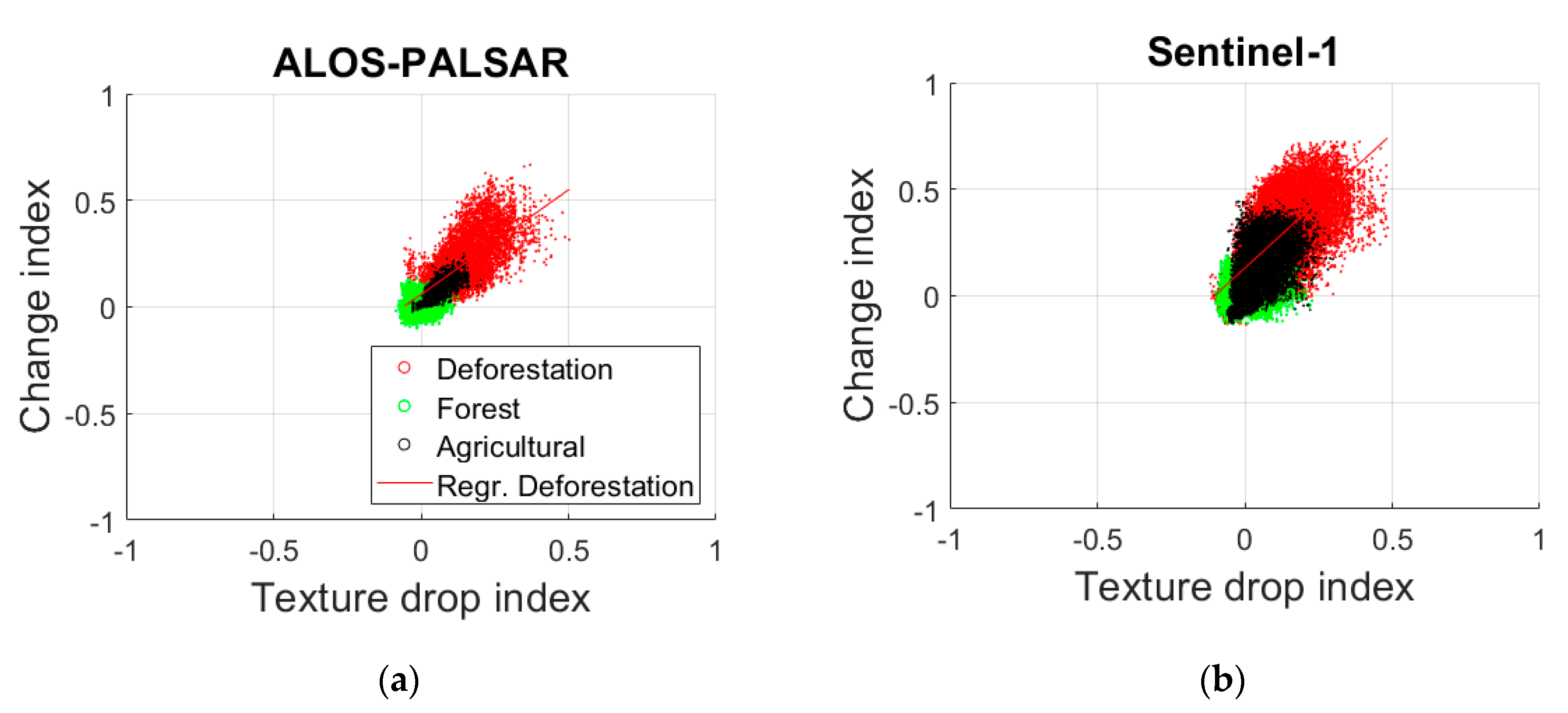
4.1. Forestry
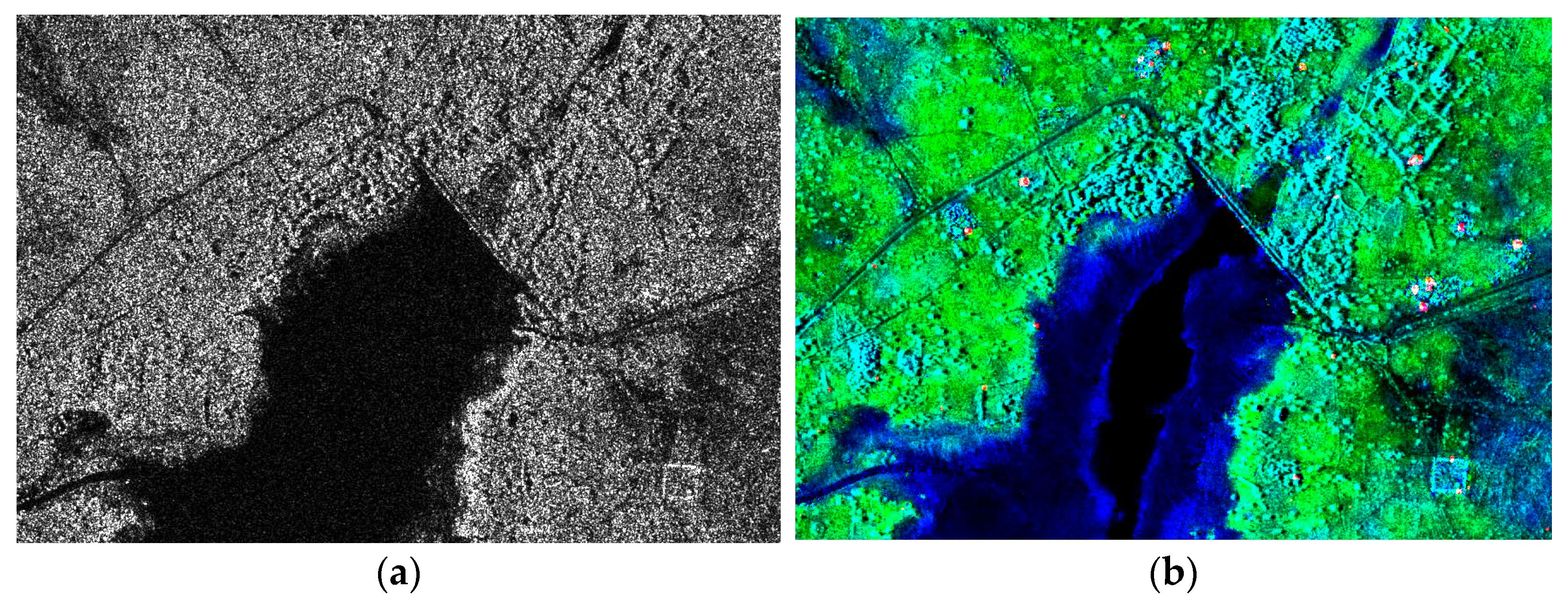
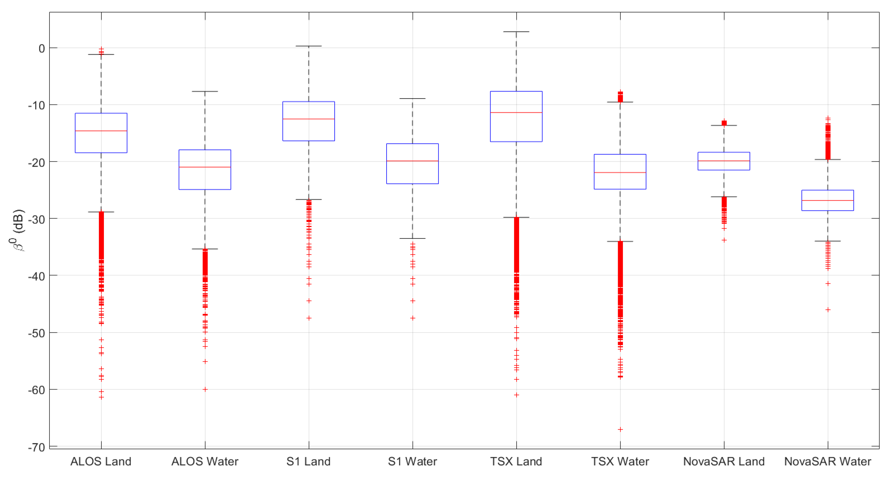
4.2. Water Resources
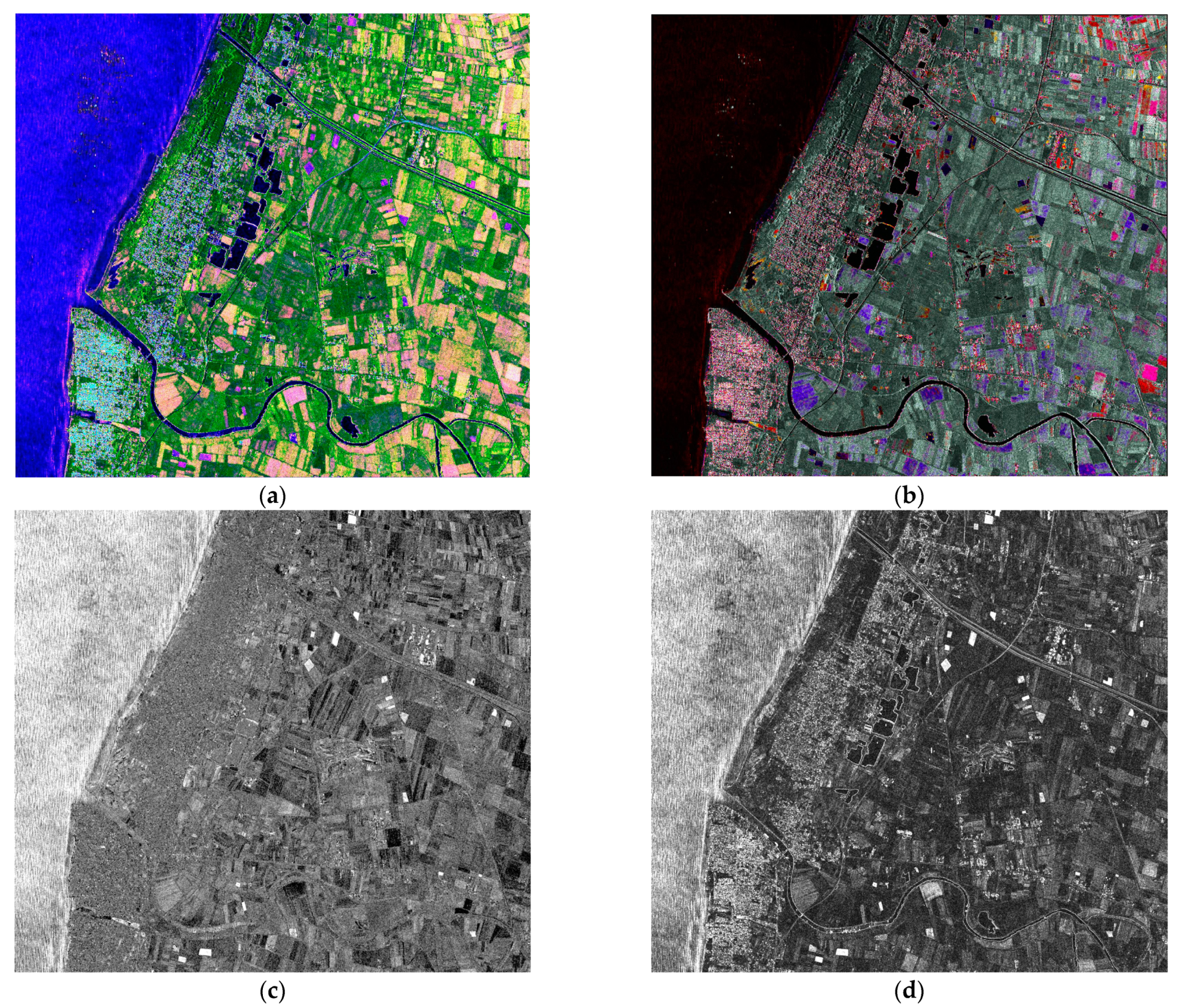
4.3. Flood Mapping
5. Discussion

6. Conclusions
Author Contributions
Funding
Data Availability Statement
Acknowledgments
Conflicts of Interest
References
- Campbell, J.B.; Wynne, R.H. Introduction to Remote Sensing; The Guilford Press: New York, NY, USA, 2011. [Google Scholar]
- Moreira, A.; Prats-Iraola, P.; Younis, M.; Krieger, G.; Hajnsek, I.; Papathanassiou, K.P. A tutorial on synthetic aperture radar. IEEE Geosci. Remote Sens. Mag. 2013, 1, 6–43. [Google Scholar] [CrossRef]
- Srivastava, P.K.; Malhi, R.K.M.; Pandey, P.C.; Akash Anand, P.; Singh, M.K.; Pandey, A.G. Revisiting hyperspectral remote sensing: Origin, processing, applications and way forward. In Hyperspectral Remote Sensing; Pandey, P.C., Srivastava, P.K., Balzter, H., Bhattacharya, B., Petropoulos, G.P., Eds.; Elsevier: Amsterdam, The Netherlands, 2020; pp. 3–21. [Google Scholar]
- Giardino, C.; Bresciani, M.; Braga, F.; Fabbretto, A.; Ghirardi, N.; Pepe, M.; Gianinetto, M.; Colombo, R.; Cogliati, S.; Ghebrehiwot, S.; et al. First Evaluation of PRISMA Level 1 Data for Water Applications. Sensors 2020, 20, 4553. [Google Scholar] [CrossRef]
- Amitrano, D.; Di Martino, G.; Iodice, A.; Riccio, D.; Ruello, G. A New Framework for SAR Multitemporal Data RGB Representation: Rationale and Products. IEEE Trans. Geosci. Remote Sens. 2015, 53, 117–133. [Google Scholar] [CrossRef]
- McFeeters, S.K. The use of the Normalized Difference Water Index (NDWI) in the delineation of open water features. Int. J. Remote Sens. 1996, 17, 1425–1432. [Google Scholar] [CrossRef]
- Carlson, T.C.; Ripley, D.A. On the relationship between NDVI, fractional vegetation cover, and leaf area index. Remote Sens. Environ. 1997, 62, 241–252. [Google Scholar] [CrossRef]
- Di Martino, G.; Iodice, A. Maritime Surveillance with Synthetic Aperture Radar; IET Digital Library: London, UK, 2020; Available online: https://shop.theiet.org/maritime-surveillance-with-synthetic-aperture-radar (accessed on 1 February 2020).
- Lanari, R.; Mora, O.; Manunta, M.; Mallorqui, J.; Berardino, P.; Sansosti, E. A small-baseline approach for investigating deformations on full-resolution differential SAR interferograms. IEEE Trans. Geosci. Remote Sens. 2004, 42, 1377–1386. [Google Scholar] [CrossRef]
- Taubenböck, H.; Esch, T.; Felbier, A.; Wiesner, M.; Roth, A.; Dech, S. Monitoring urbanization in mega cities from space. Remote Sens. Environ. 2012, 117, 162–176. [Google Scholar] [CrossRef]
- Cecinati, F.; Amitrano, D.; Leoncio, L.B.; Walugendo, E.; Guida, R.; Iervolino, P.; Natarajan, S. Exploitation of ESA and NASA Heritage Remote Sensing Data for Monitoring the Heat Island Evolution in Chennai with the Google Earth Engine. In Proceedings of the IEEE Geoscience and Remote Sensing Symposium, Yokohama, Japan, 28 July–2 August 2019; pp. 6328–6331. [Google Scholar]
- Ban, Y.; Jacob, A. Fusion of Multitemporal Spaceborne SAR and Optical Data for Urban Mapping and Urbanization Monitoring. In Multitemporal Remote Sensing. Remote Sensing and Digital Image Processing; Ban, Y., Ed.; Springer: Berlin/Heidelberg, Germany, 2016; Volume 20, ISBN 978-3-319-47035-1. [Google Scholar]
- Bargiel, D.; Herrmann, S. Multi-temporal land-cover classification of agricultural areas in two European regions with high resolution spotlight TerraSAR-X data. Remote Sens. 2011, 3, 859–877. [Google Scholar] [CrossRef]
- Kayabol, K.; Zerubia, J. Unsupervised amplitude and texture classification of SAR images with multinomial latent model. IEEE Trans. Image Process. 2013, 22, 561–572. [Google Scholar] [CrossRef]
- Amitrano, D.; Cecinati, F.; Di Martino, G.; Iodice, A.; Mathieu, P.-P.P.-P.; Riccio, D.; Ruello, G. Multitemporal Level-1β Products: Definitions, Interpretation, and Applications. IEEE Trans. Geosci. Remote Sens. 2016, 54, 6545–6562. [Google Scholar] [CrossRef]
- Di Martire, D.; Paci, M.; Confuorto, P.; Costabile, S.; Guastaferro, F.; Verta, A.; Calcaterra, D. A nation-wide system for landslide mapping and risk management in Italy: The second Not-ordinary Plan of Environmental Remote Sensing. Int. J. Appl. Earth Obs. Geoinf. 2017, 63, 143–157. [Google Scholar] [CrossRef]
- Di Martire, D.; Iglesias, R.; Monells, D.; Centolanza, G.; Sica, S.; Ramondini, M.; Pagano, L.; Mallorqui, J.; Calcaterra, D. Comparison between Differential SAR interferometry and ground measurements data in the displacement monitoring of the earth-dam of Conza della Campania (Italy). Remote Sens. Environ. 2014, 148, 58–69. [Google Scholar] [CrossRef]
- Tapete, D.; Cigna, F. InSAR data for geohazard assessment in UNESCO World Heritage sites: State-of-the-art and perspectives in the Copernicus era. Int. J. Appl. Earth Obs. Geoinf. 2017, 63, 24–32. [Google Scholar] [CrossRef]
- Strozzi, T.; Luckman, A.; Murray, T.; Wegmüller, U.; Werner, C.L. Glacier motion estimation using SAR offset-tracking procedures. IEEE Trans. Geosci. Remote Sens. 2002, 40, 2384–2391. [Google Scholar] [CrossRef]
- Amitrano, D.; Guida, R.; Di Martino, G.; Iodice, A. Glacier monitoring using frequency domain offset tracking applied to sentinel-1 images: A product performance comparison. Remote Sens. 2019, 11, 1322. [Google Scholar] [CrossRef]
- Amitrano, D.; Guida, R.; Dell’Aglio, D.; Di Martino, G.; Di Martire, D.; Iodice, A.; Costantini, M.; Malvarosa, F.; Minati, F. Long-Term Satellite Monitoring of the Slumgullion Landslide Using Space-Borne Synthetic Aperture Radar Sub-Pixel Offset Tracking. Remote Sens. 2019, 11, 369. [Google Scholar] [CrossRef]
- Datcu, M.; Seidel, K. Human-Centered Concepts for Exploration and Understanding of Earth Observation Images. IEEE Trans. Geosci. Remote Sens. 2005, 43, 601–609. [Google Scholar] [CrossRef]
- Madhok, V.; Landgrebe, D.A. A Process Model for Remote Sensing Data Analysis. IEEE Trans. Geosci. Remote Sens. 2002, 40, 680–686. [Google Scholar] [CrossRef]
- Amitrano, D.; Guida, R.; Ruello, G. Multitemporal SAR RGB Processing for Sentinel-1 GRD Products: Methodology and Applications. IEEE J. Sel. Top. Appl. Earth Obs. Remote Sens. 2019, 12, 1497–1507. [Google Scholar] [CrossRef]
- Mendel, J.M. Fuzzy Logic Systems for Engineering: A Tutorial. Proc. IEEE 1995, 83, 345–377. [Google Scholar] [CrossRef]
- Santini, S.; Gupta, A.; Jain, R. Emergent semantics through interaction in image databases. IEEE Trans. Knowl. Data Eng. 2001, 13, 337–351. [Google Scholar] [CrossRef]
- Atkin, A. Peirce’s Theory of Signs; Zalta, E.N., Ed.; The Stanford Encyclopedia of Philosophy: Stanford, CA, USA, 2013; Available online: https://plato.stanford.edu/ (accessed on 2 March 2020).
- Marr, D. Vision; W. H. Freeman: San Francisco, CA, USA, 1982. [Google Scholar]
- Esch, T.; Thiel, M.; Schenk, A.; Roth, A.; Muller, A. Delineation of Urban Footprints From TerraSAR-X Data by Analyzing Speckle Characteristics and Intensity Information. IEEE Trans. Geosci. Remote Sens. 2003, 48, 905–916. [Google Scholar] [CrossRef]
- Freeman, A. SAR Calibration: An Overview. IEEE Trans. Geosci. Remote Sens. 1992, 30, 1107–1121. [Google Scholar] [CrossRef]
- Italian Space Agency. COSMO-SkyMed Mission and Products Description; IEEE: New York, NY, USA, 2019. [Google Scholar]
- Infoterra Radiometric Calibration of TerraSAR-X Data. 2008. Available online: https://www.asi.it/wp-content/uploads/2019/08/COSMO-SkyMed-Mission-and-Products-Description_rev3-2.pdf (accessed on 1 June 2020).
- Torre, A.; Calabrese, D.; Porfilio, M. COSMO-SkyMed: Image quality achievements. In Proceedings of the 5th International Conference on Recent Advances in Space Technologies—RAST2011, Instanbal, Turkey, 9–11 June 2011; pp. 861–864. [Google Scholar]
- Schwerdt, M.; Schmidt, K.; Ramon, N.T.; Klenk, P.; Yague-Martinez, N.; Prats-Iraola, P.; Zink, M.; Geudtner, D. Independent system calibration of Sentinel-1B. Remote Sens. 2017, 9, 511. [Google Scholar] [CrossRef]
- Franceschetti, G.; Lanari, R. Synthetic Aperture Radar Processing; CRC Press: Boca Raton, FL, USA, 1999. [Google Scholar]
- Di Martino, G.; Poderico, M.; Poggi, G.; Riccio, D.; Verdoliva, L. Benchmarking Framework for SAR Despeckling. IEEE Trans. Geosci. Remote Sens. 2014, 52, 1596–1615. [Google Scholar] [CrossRef]
- De Grandi, G.F.; Leysen, M.; Lee, J.S.; Schuler, D. Radar reflectivity estimation using multiple SAR scenes of the same target: Technique and applications. In Proceedings of the IEEE International Geoscience and Remote Sensing Symposium, San Diego, CA, USA, 27 July–1 August 1997; pp. 1047–1050. [Google Scholar]
- Yu, Y.; Acton, S.T. Speckle Reducing Anisotropic Diffusion. IEEE Trans. Image Process. 2002, 11, 1260–1270. [Google Scholar]
- Su, X.; Deledalle, C.; Tupin, F.; Sun, H. Two-Step Multitemporal Nonlocal Means for Synthetic Aperture Radar Images. IEEE Trans. Geosci. Remote Sens. 2014, 52, 6181–6196. [Google Scholar]
- Cozzolino, D.; Verdoliva, L.; Scarpa, G.; Poggi, G. Nonlocal SAR Image Despeckling by Convolutional Neural Networks. In Proceedings of the IEEE International Geoscience and Remote Sensing Symposium, Yokohama, Japan, 28 July–2 August 2019; pp. 5117–5120. [Google Scholar]
- Wang, P.; Zhang, H.; Patel, V.M. SAR Image Despeckling Using a Convolutional Neural Network. IEEE Signal Process. Lett. 2017, 24, 1763–1767. [Google Scholar] [CrossRef]
- Cao, X.; Ji, Y.; Wang, L.; Ji, B.; Jiao, L.; Han, J. SAR image change detection based on deep denoising and CNN. IET Image Process. 2019, 13, 1509–1515. [Google Scholar] [CrossRef]
- Ferraioli, G.; Pascazio, V.; Vitale, S. A Novel Cost Function for Despeckling using Convolutional Neural Networks. In Proceedings of the 2019 Joint Urban Remote Sensing Event (JURSE), Vannes, France, 22–24 May 2019. [Google Scholar]
- Singh, A. Digital change detection techniques using remotely-sensed data. Int. J. Remote Sens. 1989, 10, 989–1003. [Google Scholar] [CrossRef]
- Lu, D.; Mausel, P.; Brondízio, E.; Moran, E. Change detection techniques. Int. J. Remote Sens. 2004, 25, 2365–2407. [Google Scholar] [CrossRef]
- Lee, J.S.; Jurkevich, I. Segmentation of SAR images. IEEE Trans. Geosci. Remote Sens. 1989, 27, 674–680. [Google Scholar] [CrossRef]
- Bruzzone, L.; Prieto, D.F. Automatic analysis of the difference image for unsupervised change detection. IEEE Trans. Geosci. Remote Sens. 2000, 38, 1171–1182. [Google Scholar] [CrossRef]
- Bovolo, F.; Bruzzone, L. The Time Variable in Data Fusion: A Change Detection Perspective. IEEE Geosci. Remote Sens. Mag. 2015, 3, 8–26. [Google Scholar] [CrossRef]
- Rignot, E.J.M.; Zyl, J.J. Change Detection Techniques for ERS-1 SAR Data. IEEE Trans. Geosci. Remote Sens. 1993, 31, 896–906. [Google Scholar] [CrossRef]
- Bazi, Y.; Bruzzone, L.; Melgani, F. An Unsupervised Approach Based on the Generalized Gaussian Model to Automatic Change Detection in Multitemporal SAR Images. IEEE Trans. Geosci. Remote Sens. 2005, 43, 874–887. [Google Scholar] [CrossRef]
- Grover, K.; Quegan, S.; Da Costa Freitas, C. Quantitative estimation of tropical forest cover by SAR. IEEE Trans. Geosci. Remote Sens. 1999, 37, 479–490. [Google Scholar] [CrossRef]
- Bovolo, F.; Bruzzone, L. A Detail-Preserving Scale-Driven Approach to Change Detection in Multitemporal SAR Images. IEEE Trans. Geosci. Remote Sens. 2005, 43, 2963–2972. [Google Scholar] [CrossRef]
- Amitrano, D.; Di Martino, G.; Iodice, A.; Riccio, D.; Ruello, G. Small Reservoirs Extraction in Semiarid Regions Using Multitemporal Synthetic Aperture Radar Images. IEEE J. Sel. Top. Appl. Earth Obs. Remote Sens. 2017, 10, 3482–3492. [Google Scholar] [CrossRef]
- Cian, F.; Marconcini, M.; Ceccato, P. Normalized Difference Flood Index for rapid flood mapping: Taking advantage of EO big data. Remote Sens. Environ. 2018, 209, 712–730. [Google Scholar] [CrossRef]
- Inglada, J.; Mercier, G. A New Statistical Similarity Measure for Change Detection in Multitemporal SAR Images and Its Extension to Multiscale Change Analysis. IEEE Trans. Geosci. Remote Sens. 2007, 45, 1432–1445. [Google Scholar] [CrossRef]
- Aiazzi, B.; Alparone, L.; Baronti, S.; Garzelli, A.; Zoppetti, C. Nonparametric Change Detection in Multitemporal SAR Images Based on Mean-Shift Clustering. IEEE Trans. Geosci. Remote Sens. 2013, 51, 2022–2031. [Google Scholar] [CrossRef]
- Lombardo, P.; Oliver, C.J. Maximum likelihood approach to the detection of changes between multitemporal SAR images. IEE Proc. Radar Sonar Navig. 2001, 148, 200–210. [Google Scholar] [CrossRef]
- Xiong, B.; Chen, J.M.; Kuang, G. A change detection measure based on a likelihood ratio and statistical properties of SAR intensity images. Remote Sens. Lett. 2012, 3, 267–275. [Google Scholar] [CrossRef]
- Su, X.; Deledalle, C.; Tupin, F.; Sun, H. NORCAMA: Change Analysis in SAR Time Series by Likelihood Ratio Change Matrix Clustering. ISPRS J. Photogramm. Remote Sens. 2015, 101, 247–261. [Google Scholar] [CrossRef]
- Conradsen, K.; Nielsen, A.; Schou, J.; Skriver, H. A test statistic in the complex wishart distribution and its application to change detection in polarimetric SAR data. IEEE Trans. Geosci. Remote Sens. 2003, 41, 4–19. [Google Scholar] [CrossRef]
- Otsu, N. A threshold section method from gray-level histograms. IEEE Trans. Syst. Man. Cybern. 1979, 9, 62–66. [Google Scholar] [CrossRef]
- Bazi, Y.; Bruzzone, L.; Melgani, F. Automatic identification of the number and values of decision thresholds in the log-ratio image for change detection in SAR images. IEEE Geosci. Remote Sens. Lett. 2006, 3, 349–353. [Google Scholar] [CrossRef]
- Moser, G.; Serpico, S.B. Generalized Minimum-Error Thresholding for Unsupervised Change Detection From SAR Amplitude Imagery. IEEE Trans. Geosci. Remote Sens. 2006, 44, 2972–2982. [Google Scholar] [CrossRef]
- Zhao, J.; Yang, J.; Lu, Z.; Li, P.; Liu, W.; Yang, L. A novel method of change detection in bi-temporal PolSAR data using a joint-classification classifier based on a similarity measure. Remote Sens. 2017, 9, 846. [Google Scholar] [CrossRef]
- Martinez, J.; Le Toan, T. Mapping of flood dynamics and spatial distribution of vegetation in the Amazon floodplain using multitemporal SAR data. Remote Sens. Environ. 2007, 108, 209–223. [Google Scholar] [CrossRef]
- Bujor, F.; Trouvé, E.; Valet, L.; Nicolas, J.-M.M.; Rudant, J.-P.P. Application of Log-Cumulants to the Detection of Spatiotemporal Discontinuities in Multitemporal SAR Images. IEEE Trans. Geosci. Remote Sens. 2004, 42, 2073–2084. [Google Scholar] [CrossRef]
- Ghamisi, P.; Rasti, B.; Yokoya, N.; Wang, Q.; Hofle, B.; Bruzzone, L.; Bovolo, F.; Chi, M.; Anders, K.; Gloaguen, R.; et al. Multisource and multitemporal data fusion in remote sensing: A comprehensive review of the state of the art. IEEE Geosci. Remote Sens. Mag. 2019, 7, 6–39. [Google Scholar] [CrossRef]
- Pohl, C.; Van Genderen, J.L. Review Article Multisensor Image Fusion in Remote Sensing: Concepts, Methods and Applications. Int. J. Remote Sens. 1998, 19, 823–854, ISBN 0143116982157. [Google Scholar] [CrossRef]
- Lehmann, E.A.; Caccetta, P.A.; Zhou, Z.S.; McNeill, S.J.; Wu, X.; Mitchell, A.L. Joint processing of landsat and ALOS-PALSAR data for forest mapping and monitoring. IEEE Trans. Geosci. Remote Sens. 2012, 50, 55–67. [Google Scholar] [CrossRef]
- Reiche, J.; Verbesselt, J.; Hoekman, D.; Herold, M. Fusing Landsat and SAR time series to detect deforestation in the tropics. Remote Sens. Environ. 2015, 156, 276–293. [Google Scholar] [CrossRef]
- Poulain, V.; Inglada, J.; Spigai, M.; Tourneret, J.Y.; Marthon, P. High-resolution optical and SAR image fusion for building database updating. IEEE Trans. Geosci. Remote Sens. 2011, 49, 2900–2910. [Google Scholar] [CrossRef]
- Smets, P. What is Dempster-Shafer’s model? In Advances in the Dempster-Shafer Theory of Evidence; John Wiley & Sons, Inc.: New York, NY, USA, 1994; pp. 5–34. [Google Scholar]
- Brunner, D.; Lemoine, G.; Bruzzone, L. Earthquake Damage Assessment of Buildings Using VHR Optical and SAR Imagery. IEEE Trans. Geosci. Remote Sens. 2010, 48, 2403–2420. [Google Scholar] [CrossRef]
- Errico, A.; Angelino, C.V.; Cicala, L.; Persechino, G.; Ferrara, C.; Lega, M.; Vallario, A.; Parente, C.; Masi, G.; Gaetano, R.; et al. Detection of environmental hazards through the feature-based fusion of optical and SAR data: A case study in southern Italy. Int. J. Remote Sens. 2015, 36, 3345–3367. [Google Scholar] [CrossRef]
- Polychronaki, A.; Gitas, I.Z.; Veraverbeke, S.; Debien, A. Evaluation of ALOS PALSAR imagery for burned area mapping in greece using object-based classification. Remote Sens. 2013, 5, 5680–5701. [Google Scholar] [CrossRef]
- Blaschke, T. Object based image analysis for remote sensing. ISPRS J. Photogramm. Remote Sens. 2010, 65, 2–16. [Google Scholar] [CrossRef]
- Amitrano, D.; Cecinati, F.; Di Martino, G.; Iodice, A.; Mathieu, P.-P.; Riccio, D.; Ruello, G. Feature Extraction From Multitemporal SAR Images Using Selforganizing Map Clustering and Object-Based Image Analysis. IEEE J. Sel. Top. Appl. Earth Obs. Remote Sens. 2018, 11, 1556–1570. [Google Scholar] [CrossRef]
- Amitrano, D.; Di Martino, G.; Iodice, A.; Riccio, D.; Ruello, G. RGB SAR products: Methods and applications. Eur. J. Remote Sens. 2016, 49, 777–793. [Google Scholar] [CrossRef]
- Salentinig, A.; Gamba, P. A General Framework for Urban Area Extraction Exploiting Multiresolution SAR Data Fusion. IEEE J. Sel. Top. Appl. Earth Obs. Remote Sens. 2016, 9, 2009–2018. [Google Scholar] [CrossRef]
- Landuyt, L.; Van Wesemael, A.; Schumann, G.J.P.; Hostache, R.; Verhoest, N.E.C.; Van Coillie, F.M.B. Flood Mapping Based on Synthetic Aperture Radar: An Assessment of Established Approaches. IEEE Trans. Geosci. Remote Sens. 2019, 57, 722–739. [Google Scholar] [CrossRef]
- Saatchi, S.S.; Soares, J.V.; Alves, D.S. Mapping deforestation and land use in Amazon rainforest by using SIR-C imagery. Remote Sens. Environ. 1997, 59, 191–202. [Google Scholar] [CrossRef]
- Amitrano, D.; Ciervo, F.; Di Martino, G.; Papa, M.N.; Iodice, A.; Koussoube, Y.; Mitidieri, F.; Riccio, D.; Ruello, G. Modeling Watershed Response in Semiarid Regions With High-Resolution Synthetic Aperture Radars. IEEE J. Sel. Top. Appl. Earth Obs. Remote Sens. 2014, 7, 2732–2745. [Google Scholar] [CrossRef]
- Milillo, P.; Fielding, E.J.; Shulz, W.H.; Delbridge, B.; Burgmann, R. COSMO-SkyMed spotlight interferometry over rural areas: The slumgullion landslide in Colorado, USA. IEEE J. Sel. Top. Appl. Earth Obs. Remote Sens. 2014, 7, 2919–2926. [Google Scholar] [CrossRef]
- Wang, C.; Mao, X.; Wang, Q. Landslide displacement monitoring by a fully polarimetric SAR offset tracking method. Remote Sens. 2016, 8, 624. [Google Scholar] [CrossRef]
- Lemos, A.; Shepherd, A.; McMillan, M.; Hogg, A.E.; Hatton, E.; Joughin, I. Ice velocity of Jakobshavn Isbræ, Petermann Glacier, Nioghalvfjerdsfjorden, and Zachariæ Isstrøm, 2015–2017, from Sentinel 1-a/b SAR imagery. Cryosphere 2018, 12, 2087–2097. [Google Scholar] [CrossRef]
- Dellepiane, S.G.; Angiati, E. A New Method for Cross-Normalization and Multitemporal Visualization of SAR Images for the Detection of Flooded Areas. IEEE Trans. Geosci. Remote Sens. 2012, 50, 2765–2779. [Google Scholar] [CrossRef]
- Nakmuenwai, P.; Yamazaki, F.; Liu, W. Multi-Temporal Correlation Method for Damage Assessment of Buildings from High-Resolution SAR Images of the 2013 Typhoon Haiyan. J. Disaster Res. 2016, 11, 577–592. [Google Scholar] [CrossRef]
- Refice, A.; Capolongo, D.; Pasquariello, G.; D’Addabbo, A.; Bovenga, F.; Nutricato, R.; Lovergine, F.P.; Pietranera, L. SAR and InSAR for Flood Monitoring: Examples with COSMO-SkyMed Data. IEEE J. Sel. Top. Appl. Earth Obs. Remote Sens. 2014, 7, 2711–2722. [Google Scholar] [CrossRef]
- Amitrano, D.; Cecinati, F.; Di Martino, G.; Iodice, A.; Mathieu, P.-P.; Riccio, D.; Ruello, G. An end-user-oriented framework for RGB representation of multitemporal SAR images and visual data mining. In Proceedings of the SPIE Remote Sensing, Edinburgh, UK, 26–28 September 2016; Volume 10004. [Google Scholar]
- Alves, E.I.; Andrade, A.I.A.S.S.; Vaz, D.A. A Better View over Titan Drainage Networks Through RGB Fusion of Cassini SAR Images. IEEE Geosci. Remote Sens. Lett. 2018, 15, 414–418. [Google Scholar] [CrossRef]
- Perrou, T.; Garioud, A.; Parcharidis, I. Use of Sentinel-1 imagery for flood management in a reservoir-regulated river basin. Front. Earth Sci. 2018, 12, 506–520. [Google Scholar] [CrossRef]
- Schmitt, M.; Hughes, L.H.; Körner, M.; Zhu, X.X. Colorizing sentinel-1 SAR images using a variational autoencoder conditioned on Sentinel-2 imagery. In Proceedings of the International Archives of the Photogrammetry, Remote Sensing and Spatial Information Sciences, Riva del Garda, Italy, 4–7 June 2018; Volume 42, pp. 1045–1051. [Google Scholar]
- Colin-Koeniguer, E.; Boulch, A.; Trouvé-Peloux, P.; Janez, F. Colored visualization of multitemporal SAR data for change detection: Issues and methods. In Proceedings of the EUSAR 2018, 12th European Conference on Synthetic Aperture Radar, Aachen, Germany, 4–7 June 2018; pp. 1038–1041. [Google Scholar]
- Haralick, R.M.; Shanmugam, K.; Dinstein, I.H. Textural Features for Image Classification. IEEE Trans. Syst. Man Cybern. 1973, SMC-3, 610–621. [Google Scholar] [CrossRef]
- Amitrano, D.; Di Martino, G.; Iodice, A.; Riccio, D.; Ruello, G. Unsupervised Rapid Flood Mapping Using Sentinel-1 GRD SAR Images. IEEE Trans. Geosci. Remote Sens. 2018, 56, 3290–3299. [Google Scholar] [CrossRef]
- Fung, A.K. Scattering from a Vegetation Layer. IEEE Trans. Geosci. Electron. 1979, 17, 1–6. [Google Scholar] [CrossRef]
- Khellaf, A.; Beghdadi, A.; Dupoisot, H. Entropic Contrast Enhancement. IEEE Trans. Med. Imaging 1991, 10, 589–592. [Google Scholar] [CrossRef]
- Jacobson, N.P.; Gupta, M.R.; Cole, J.B. Linear Fusion of Image Sets for Display. IEEE Trans. Geosci. Remote Sens. 2007, 45, 3277–3288. [Google Scholar] [CrossRef]
- Healey, C.G.; Booth, K.S.; Enns, J.T. Visualizing real-time multivariate data using preattentive processing. ACM Trans. Model. Comput. Simul. 1995, 5, 190–221. [Google Scholar] [CrossRef]
- Mitchard, E.T.A. The tropical forest carbon cycle and climate change. Nature 2018, 559, 527–534. [Google Scholar] [CrossRef]
- Waring, R.H.; Running, S.W. Forest Ecosystems Analysis at Multiple Scales; Elsevier: Amsterdam, The Netherlands, 2007; ISBN 9780123706058. [Google Scholar]
- Battaglia, M.; Sands, P.J. Process-based forest productivity models and their application in forest management. For. Ecol. Manag. 1998, 102, 13–32. [Google Scholar] [CrossRef]
- Wolter, P.T.; Mladenoff, D.J.; Host, G.E.; Crow, T.R. Improved forest classification in the northern Lake States using multitemporal Landsat imagery. Photogramm. Eng. Rem. Sens. 1995, 61, 1129–1143. [Google Scholar]
- Holmgren, P.; Thuresson, T. Satellite remote sensing for forestry planning—A review. Scand. J. For. Res. 1998, 13, 90–110. [Google Scholar] [CrossRef]
- Iverson, L.R.; Graham, R.L.; Cook, E.A. Applications of satellite remote sensing to forested ecosystems. Landsc. Ecol. 1989, 3, 131–143. [Google Scholar] [CrossRef]
- Cohen, W.B.; Kushla, J.D.; Ripple, W.J.; Garman, S.L. An introduction to digital methods in remote sensing of forested ecosystems: Focus on the Pacific Northwest, USA. Environ. Manag. 1996, 20, 421–435. [Google Scholar] [CrossRef]
- Goodenough, D.G.; Bhogal, A.S.; Fournier, R.; Hall, R.J.; Iisaka, J.; Leckie, D.; Luther, J.E.; Magnussen, S.; Niemann, O.; Strome, W.M. Earth observation for sustainable development of forests (EOSD). In Proceedings of the IEEE International Geoscience and Remote Sensing Symposium, Seattle, WA, USA, 6–10 July 1998; pp. 57–60. [Google Scholar]
- Landsberg, J.; Gower, S.T. Application of Physiological Ecology to Forest Production; Academic Press: Cambridge, MA, USA, 1996. [Google Scholar]
- Lu, M.; Chen, B.; Liao, X.; Yue, T.; Yue, H.; Ren, S.; Li, X.; Nie, Z.; Xu, B. Forest types classification based on multi-source data fusion. Remote Sens. 2017, 9, 1153. [Google Scholar] [CrossRef]
- Mariotti D’Alessandro, M.; Tebaldini, S. Digital terrain model retrieval in tropical forests through P-Band SAR tomography. IEEE Trans. Geosci. Remote Sens. 2019, 57, 6774–6781. [Google Scholar] [CrossRef]
- Jha, C.S.; Goparaju, L.; Tripathi, A.; Gharai, B.; Raghubanshi, A.S.; Singh, J.S. Forest fragmentation and its impact on species diversity: An analysis using remote sensing and GIS. Biodivers. Conserv. 2005, 14, 1681–1698. [Google Scholar] [CrossRef]
- Chen, G.; Meentemeyer, R. Remote Sensing of Forest Damage by Diseases and Insects. In Remote Sensing for Sustainability; Weng, Q., Ed.; CRC Press: Boca Raton, FL, USA, 2016; pp. 145–162. [Google Scholar]
- Sunar, F.; Oezkan, C. Forest fire analysis with remote sensing data. Int. J. Remote Sens. 2001, 22, 2265–2277. [Google Scholar] [CrossRef]
- Aguilar, A. Remote Sensing of Forest Regeneration in Highland Tropical Forests. GIScience Remote Sens. 2005, 42, 66–79. [Google Scholar] [CrossRef]
- Tanase, M.A.; de la Riva, J.; Santoro, M.; Pérez-Cabello, F.; Kasischke, E. Sensitivity of SAR data to post-fire forest regrowth in Mediterranean and boreal forests. Remote Sens. Environ. 2011, 115, 2075–2085. [Google Scholar] [CrossRef]
- Kurvonen, L.; Pulliainen, J.T.; Hallikainen, M.T. Retrieval of Biomass in Boreal Forests from Multitemporal ERS-1 and JERS-1 SAR Images. IEEE Trans. Geosci. Remote Sens. 1999, 37, 198–205. [Google Scholar] [CrossRef]
- Kennedy, R.E.; Yang, Z.; Cohen, W.B. Detecting trends in forest disturbance and recovery using yearly Landsat time series: 1. LandTrendr—Temporal segmentation algorithms. Remote Sens. Environ. 2010, 114, 2897–2910. [Google Scholar] [CrossRef]
- Hansen, M.C.; Shimabukuro, Y.E.; Potapov, P.; Pittman, K. Comparing annual MODIS and PRODES forest cover change data for advancing monitoring of Brazilian forest cover. Remote Sens. Environ. 2008, 112, 3784–3793. [Google Scholar] [CrossRef]
- Diniz, C.G.; de Almeida Souza, A.A.; Santos, D.C.; Dias, M.C.; da Luz, N.C.; de Moraes, D.R.V.; Maia, J.S.A.; Gomes, A.R.; da Silva Narvaes, I.; Valeriano, D.M.; et al. DETER-B: The New Amazon Near Real-Time Deforestation Detection System. IEEE J. Sel. Top. Appl. Earth Obs. Remote Sens. 2015, 8, 3619–3628. [Google Scholar] [CrossRef]
- Hansen, M.C.; Krylov, A.; Tyukavina, A.; Potapov, P.V.; Turubanova, S.; Zutta, B.; Ifo, S.; Margono, B.; Stolle, F.; Moore, R. Humid tropical forest disturbance alerts using Landsat data. Environ. Res. Lett. 2016, 11, 034008. [Google Scholar] [CrossRef]
- Hansen, M.C.; Potapov, P.V.V.; Moore, R.; Hancher, M.; Turubanova, S.A.; Tyukavina, A.; Thau, D.; Stehman, S.V.; Goetz, S.J.; Loveland, T.R.; et al. High-Resolution Global Maps of 21st-Century Forest Cover Change. Science 2013, 850, 850–854. [Google Scholar] [CrossRef] [PubMed]
- Wylie, D.P.; Jackson, D.L.; Menzel, W.P.; Bates, J.J. Global cloud cover trends inferred from two decades of HIRS observations. J. Clim. 2005, 18, 3021–3031. [Google Scholar] [CrossRef]
- Sannier, C.; McRoberts, R.E.; Fichet, L.V. Suitability of Global Forest Change data to report forest cover estimates at national level in Gabon. Remote Sens. Environ. 2016, 173, 326–338. [Google Scholar] [CrossRef]
- Cunningham, D.; Cunningham, P.; Fagan, M.E. Identifying biases in global tree cover products: A case study in Costa Rica. Forests 2019, 10, 853. [Google Scholar] [CrossRef]
- Ulaby, F.T.; Long, D.G. Microwave Radar and Radiometric Remote Sensing; The University of Michigan Press: Ann Arbor, MI, USA, 2014. [Google Scholar]
- Hoekman, D.H. Radar backscattering of forest stands. Int. J. Remote Sens. 1985, 6, 325–343. [Google Scholar] [CrossRef]
- Westman, W.E.; Paris, J.F. Detecting forest structure and biomass with C-band multipolarization radar: Physical model and field tests. Remote Sens. Environ. 1987, 22, 249–269. [Google Scholar] [CrossRef]
- Richards, J.A.; Sun, G.; Simonett, D.S. L-Band Radar Backscatter Modeling of Forest Stands. IEEE Trans. Geosci. Remote Sens. 1987, GE-25, 487–498. [Google Scholar] [CrossRef]
- Rignot, E.J.M.; Williams, C.L.; Viereck, L.A. Mapping of Forest Types in Alaskan Boreal Forests Using SAR Imagery. IEEE Trans. Geosci. Remote Sens. 1994, 32, 1051–1059. [Google Scholar] [CrossRef]
- Ranson, K.J.; Saatchi, S.; Sun, G. Boreal Forest Ecosystem Characterization with SIR-C/XSAR. IEEE Trans. Geosci. Remote Sens. 1995, 33, 867–876. [Google Scholar] [CrossRef]
- Ranson, K.J.; Sun, G. An Evaluation of AIRSAR and SIR-C/X-SAR Images for Mapping Northern Forest Attributes in Maine, USA. Remote Sens. Environ. 1995, 59, 202–223. [Google Scholar] [CrossRef]
- Pierce, L.E.; Bergen, K.M.; Dobson, M.C.; Ulaby, F.T. Multitemporal land-cover classification using SIR-C/X-SAR imagery. Remote Sens. Environ. 1998, 64, 20–33. [Google Scholar] [CrossRef]
- Ortiz, S.M.; Breidenbach, J.; Knuth, R.; Kändler, G. The influence of DEM quality on mapping accuracy of coniferous- and deciduous-dominated forest using TerraSAR-X images. Remote Sens. 2012, 4, 661–681. [Google Scholar] [CrossRef]
- Saatchi, S.S.; Rignot, E. Classification of Boreal forest cover types using SAR images. Remote Sens. Environ. 1997, 60, 270–281. [Google Scholar] [CrossRef]
- Fassnacht, F.E.; Latifi, H.; Stereńczak, K.; Modzelewska, A.; Lefsky, M.; Waser, L.T.; Straub, C.; Ghosh, A. Review of studies on tree species classification from remotely sensed data. Remote Sens. Environ. 2016, 186, 64–87. [Google Scholar] [CrossRef]
- Shimada, M.; Itoh, T.; Motooka, T.; Watanabe, M.; Shiraishi, T.; Thapa, R.; Lucas, R. New global forest/non-forest maps from ALOS PALSAR data (2007–2010). Remote Sens. Environ. 2014, 155, 13–31. [Google Scholar] [CrossRef]
- Mermoz, S.; Le Toan, T. Forest disturbances and regrowth assessment using ALOS PALSAR data from 2007 to 2010 in Vietnam, Cambodia and Lao PDR. Remote Sens. 2016, 8, 271. [Google Scholar] [CrossRef]
- Lei, Y.; Lucas, R.; Siqueira, P.; Schmidt, M.; Treuhaft, R. Detection of forest disturbance with spaceborne repeat-pass SAR interferometry. IEEE Trans. Geosci. Remote Sens. 2018, 56, 2424–2439. [Google Scholar] [CrossRef]
- Almeida-Filho, R.; Rosenqvist, A.; Shimabukuro, Y.E.; Silva-Gomez, R. Detecting deforestation with multitemporal L-band SAR imagery: A case study in western Brazilian Amazônia. Int. J. Remote Sens. 2007, 28, 1383–1390. [Google Scholar] [CrossRef]
- Watanabe, M.; Koyama, C.N.; Hayashi, M.; Nagatani, I.; Shimada, M. Early-stage deforestation detection in the tropics with L-band SAR. IEEE J. Sel. Top. Appl. Earth Obs. Remote Sens. 2018, 11, 2127–2133. [Google Scholar] [CrossRef]
- Ryan, C.M.; Hill, T.; Woollen, E.; Ghee, C.; Mitchard, E.; Cassells, G.; Grace, J.; Woodhouse, I.H.; Williams, M. Quantifying small-scale deforestation and forest degradation in African woodlands using radar imagery. Glob. Chang. Biol. 2012, 18, 243–257. [Google Scholar] [CrossRef]
- Almeida-Filho, R.; Shimabukuro, Y.E.; Rosenqvist, A.; Sánchez, G.A. Using dual-polarized ALOS PALSAR data for detecting new fronts of deforestation in the Brazilian Amazônia. Int. J. Remote Sens. 2009, 30, 3735–3743. [Google Scholar] [CrossRef]
- Motohka, T.; Shimada, M.; Uryu, Y.; Setiabudi, B. Using time series PALSAR gamma nought mosaics for automatic detection of tropical deforestation: A test study in Riau, Indonesia. Remote Sens. Environ. 2014, 155, 79–88. [Google Scholar] [CrossRef]
- Santoro, M.; Fransson, J.E.S.; Eriksson, L.E.B.; Ulander, L.M.H. Clear-Cut Detection in Swedish Boreal Forest Using Multi-Temporal ALOS PALSAR Backscatter Data. IEEE J. Sel. Top. Appl. Earth Obs. Remote Sens. 2010, 3, 618–631. [Google Scholar] [CrossRef]
- Joshi, N.P.; Mitchard, E.T.A.; Schumacher, J.; Johannsen, V.K.; Saatchi, S.; Fensholt, R. L-Band SAR Backscatter Related to Forest Cover, Height and Aboveground Biomass at Multiple Spatial Scales across Denmark. Remote Sens. 2015, 7, 4442–4472. [Google Scholar] [CrossRef]
- Whittle, M.; Quegan, S.; Uryu, Y.; Stüewe, M.; Yulianto, K. Detection of tropical deforestation using ALOS-PALSAR: A Sumatran case study. Remote Sens. Environ. 2012, 124, 83–98. [Google Scholar] [CrossRef]
- Walker, W.S.; Kellndorfer, J.M.; Kirsch, K.M.; Stickler, C.M.; Nepstad, D.C.; Stickler, C.M.; Nepstad, D.C. Large-Area Classification and Mapping of Forest and Land Cover in the Brazilian Amazon: A Comparative Analysis of ALOS/PALSAR and Landsat Data Sources. IEEE J. Sel. Top. Appl. Earth Obs. Remote Sens. 2010, 3, 594–604. [Google Scholar] [CrossRef]
- Reiche, J.; Souzax, C.M.; Hoekman, D.H.; Verbesselt, J.; Persaud, H.; Herold, M. Feature level fusion of multi-temporal ALOS PALSAR and Landsat data for mapping and monitoring of tropical deforestation and forest degradation. IEEE J. Sel. Top. Appl. Earth Obs. Remote Sens. 2013, 6, 2159–2173. [Google Scholar] [CrossRef]
- Wegmüller, U.; Werner, C.L. SAR Interferometric Signatures of Forest. IEEE Trans. Geosci. Remote Sens. 1995, 33, 1153–1161. [Google Scholar] [CrossRef]
- Quegan, S.; Le Toan, T.; Yu, J.J.; Ribbes, F.; Floury, N.; Le Toan, T.; Yu, J.J.; Ribbes, F.; Floury, N. Multitemporal ERS SAR analysis applied to forest mapping. IEEE Trans. Geosci. Remote Sens. 2000, 38, 741–753. [Google Scholar] [CrossRef]
- Hoekman, D. Monitoring Tropical Peat Swamp Deforestation and Hydrological Dynamics by ASAR and PALSAR. In Geoscience and Remote Sensing; Ho, P.-G., Ed.; IntechOpen: London, UK, 2009. [Google Scholar]
- Bouvet, A.; Mermoz, S.; Ballère, M.; Koleck, T.; Le Toan, T. Use of the SAR Shadowing Effect for Deforestation Detection with Sentinel-1 Time Series. Remote Sens. 2018, 10, 1250. [Google Scholar] [CrossRef]
- Lohberger, S.; Stängel, M.; Atwood, E.C.; Siegert, F. Spatial evaluation of Indonesia’s 2015 fire-affected area and estimated carbon emissions using Sentinel-1. Glob. Chang. Biol. 2018, 24, 644–654. [Google Scholar] [CrossRef]
- Reiche, J.; Hamunyela, E.; Verbesselt, J.; Hoekman, D.; Herold, M. Improving near-real time deforestation monitoring in tropical dry forests by combining dense Sentinel-1 time series with Landsat and ALOS-2 PALSAR-2. Remote Sens. Environ. 2018, 204, 147–161. [Google Scholar] [CrossRef]
- Sica, F.; Pulella, A.; Rizzoli, P.; Aerospace, G.; Straße, M. Forest Classification and Deforestation Mapping By Means of Sentinel-1. In Proceedings of the IGARSS 2019—2019 IEEE International Geoscience and Remote Sensing Symposium, Yokohama, Japan, 28 July–2 August 2019; pp. 2635–2638. [Google Scholar]
- Schlund, M.; von Poncet, F.; Hoekman, D.H.; Kuntz, S.; Schmullius, C. Importance of bistatic SAR features from TanDEM-X for forest mapping and monitoring. Remote Sens. Environ. 2014, 151, 16–26. [Google Scholar] [CrossRef]
- Martone, M.; Rizzoli, P.; Wecklich, C.; González, C.; Bueso-Bello, J.L.; Valdo, P.; Schulze, D.; Zink, M.; Krieger, G.; Moreira, A. The global forest/non-forest map from TanDEM-X interferometric SAR data. Remote Sens. Environ. 2018, 205, 352–373. [Google Scholar] [CrossRef]
- Bird, R.; Whittaker, P.; Stern, B.; Angli, N.; Cohen, M.; Guida, R. NovaSAR-S a low cost approach to sar applications, synthetic aperture radar. In Proceedings of the IEEE 2013 Asia-Pacific Conference on Synthetic Aperture Radar (APSAR), Tsukuba, Japan, 23–27 September 2013. [Google Scholar]
- Ningthoujam, R.K.; Tansey, K.; Balzter, H.; Morrison, K.; Johnson, S.C.M.; Gerard, F.; George, C.; Burbidge, G.; Doody, S.; Veck, N.; et al. Mapping forest cover and forest cover change with airborne S-band radar. Remote Sens. 2016, 8, 577. [Google Scholar] [CrossRef]
- Sun, G.; Ranson, K.J. Radar modelling of forest spatial patterns. Int. J. Remote Sens. 1998, 19, 1769–1791. [Google Scholar] [CrossRef]
- Kuplich, T.M.; Curran, P.J.; Atkinson, P.M. Relating SAR image texture to the biomass of regenerating tropical forests. Int. J. Remote Sens. 2005, 26, 4829–4854. [Google Scholar] [CrossRef]
- Englhart, S.; Keuck, V.; Siegert, F. Modeling aboveground biomass in tropical forests using multi-frequency SAR data-A comparison of methods. IEEE J. Sel. Top. Appl. Earth Obs. Remote Sens. 2012, 5, 298–306. [Google Scholar] [CrossRef]
- Yu, Y.; Saatchi, S. Sensitivity of L-band SAR backscatter to aboveground biomass of global forests. Remote Sens. 2016, 8, 522. [Google Scholar] [CrossRef]
- Mermoz, S.; Réjou-Méchain, M.; Villard, L.; Le Toan, T.; Rossi, V.; Gourlet-Fleury, S. Decrease of L-band SAR backscatter with biomass of dense forests. Remote Sens. Environ. 2015, 159, 307–317. [Google Scholar] [CrossRef]
- Cartus, O.; Santoro, M.; Kellndorfer, J. Mapping forest aboveground biomass in the Northeastern United States with ALOS PALSAR dual-polarization L-band. Remote Sens. Environ. 2012, 124, 466–478. [Google Scholar] [CrossRef]
- Lucas, R.; Bunting, P.; Clewley, D.; Armston, J.; Fairfax, R.; Fensham, R.; Accad, A.; Kelley, J.; Laidlaw, M.; Eyre, T.; et al. An Evaluation of the ALOS PALSAR L-Band Backscatter—Above Ground Biomass Relationship Queensland, Australia: Impacts of Surface Moisture Condition and Vegetation Structure. IEEE J. Sel. Top. Appl. Earth Obs. Remote Sens. 2010, 3, 576–593. [Google Scholar] [CrossRef]
- Neumann, M.; Saatchi, S.S.; Ulander, L.M.H.; Fransson, J.E.S. Assessing performance of L- and P-band polarimetric interferometric SAR data in estimating boreal forest above-ground biomass. IEEE Trans. Geosci. Remote Sens. 2012, 50, 714–726. [Google Scholar] [CrossRef]
- Luckman, A.; Baker, J.; Kuplich, T.M.; Corina da Costa, F.Y.; Alejandro, C.F. A study of the relationship between radar backscatter and regenerating tropical forest biomass for spaceborne SAR instruments. Remote Sens. Environ. 1997, 60, 1–13. [Google Scholar] [CrossRef]
- Berninger, A.; Lohberger, S.; Stängel, M.; Siegert, F. SAR-based estimation of above-ground biomass and its changes in tropical forests of Kalimantan using L- and C-band. Remote Sens. 2018, 10, 831. [Google Scholar] [CrossRef]
- Laurin, G.V.; Balling, J.; Corona, P.; Mattioli, W.; Papale, D.; Puletti, N.; Rizzo, M.; Truckenbrodt, J.; Urban, M. Above-ground biomass prediction prediction by Sentinel-1 multitemporal data in central Italy with inetgration of ALOS2 and Sentinel. J. Appl. Remote Sens. 2018, 12, 16008. [Google Scholar] [CrossRef]
- Ningthoujam, R.K.; Balzter, H.; Tansey, K.; Morrison, K.; Johnson, S.C.M.; Gerard, F.; George, C.; Malhi, Y.; Burbidge, G.; Doody, S.; et al. Airborne S-band SAR for forest biophysical retrieval in temperate mixed forests of the UK. Remote Sens. 2016, 8, 609. [Google Scholar] [CrossRef]
- Ningthoujam, R.K.; Balzter, H.; Tansey, K.; Feldpausch, T.R.; Mitchard, E.T.A.; Wani, A.A.; Joshi, P.K. Relationships of S-band radar backscatter and forest aboveground biomass in different forest types. Remote Sens. 2017, 9, 1116. [Google Scholar] [CrossRef]
- Ulaby, F.T.; Sarabandi, K.; Mcdonald, K.; Whitt, M.; Dobson, M.C. Michigan microwave canopy scattering model. Int. J. Remote Sens. 1990, 11, 1223–1253. [Google Scholar] [CrossRef]
- Yatabe, S.M.; Leckie, D.G. Clearcut and forest-type discrimination in satellite SAR imagery. Can. J. Remote Sens. 1995, 21, 455–467. [Google Scholar] [CrossRef]
- Fransson, J.E.S.; Walter, F.; Olsson, H. Identification of clear felled areas using Spot P and Almaz-1 SAR data. Int. J. Remote Sens. 1999, 20, 3583–3593. [Google Scholar] [CrossRef]
- Imhoff, M.L. Radar backscatter and biomass saturation: Ramifications for global biomass inventory. IEEE Trans. Geosci. Remote Sens. 1995, 33, 511–518. [Google Scholar] [CrossRef]
- Lucas, R.M.; Cronin, N.; Lee, A.; Moghaddam, M.; Witte, C.; Tickle, P. Empirical relationships between AIRSAR backscatter and LiDAR-derived forest biomass, Queensland, Australia. Remote Sens. Environ. 2006, 100, 407–425. [Google Scholar] [CrossRef]
- Santoro, M.; Eriksson, L.; Askne, J.; Schmullius, C. Assessment of stand-wise stem volume retrieval in boreal forest from JERS-1 L-band SAR backscatter. Int. J. Remote Sens. 2006, 27, 3425–3454. [Google Scholar] [CrossRef]
- Tanase, M.A.; Kennedy, R.; Aponte, C. Fire severity estimation from space: A comparison of active and passive sensors and their synergy for different forest types. Int. J. Wildl. Fire 2015, 24, 1062–1075. [Google Scholar] [CrossRef]
- Chuvieco, E.; Mouillot, F.; van der Werf, G.R.; San Miguel, J.; Tanasse, M.; Koutsias, N.; García, M.; Yebra, M.; Padilla, M.; Gitas, I.; et al. Historical background and current developments for mapping burned area from satellite Earth observation. Remote Sens. Environ. 2019, 225, 45–64. [Google Scholar] [CrossRef]
- Kasischke, E.S.; Bourgeau-Chavez, L.L.; Johnstone, J.F. Assessing spatial and temporal variations in surface soil moisture in fire-disturbed black spruce forests in Interior Alaska using spaceborne synthetic aperture radar imagery—Implications for post-fire tree recruitment. Remote Sens. Environ. 2007, 108, 42–58. [Google Scholar] [CrossRef]
- Siegert, F.; Ruecker, G. Use of multitemporal ERS-2 SAR images for identification of burned scars in south-east Asian tropical rainforest. Int. J. Remote Sens. 2000, 21, 831–837. [Google Scholar] [CrossRef]
- Siegert, F.; Hoffmann, A.A. The 1998 Forest Fires in East Kalimantan (Indonesia): A Quantitative Evaluation Using High Resolution, Multitemporal ERS-2 SAR Images and NOAA-AVHRR Hotspot Data. Remote Sens. Environ. 1998, 72, 64–77. [Google Scholar] [CrossRef]
- Kalogirou, V.; Ferrazzoli, P.; Vecchia, A.D.; Foumelis, M. On the SAR backscatter of burned forests: A model-based study in C-band, over burned pine canopies. IEEE Trans. Geosci. Remote Sens. 2014, 52, 6205–6215. [Google Scholar] [CrossRef]
- Tanase, M.A.; Santoro, M.; Wegmüller, U.; de la Riva, J.; Pérez-Cabello, F. Properties of X-, C- and L-band repeat-pass interferometric SAR coherence in Mediterranean pine forests affected by fires. Remote Sens. Environ. 2010, 114, 2182–2194. [Google Scholar] [CrossRef]
- Bourgeau-Chavez, L.L.; Harrell, P.A.; Kasischke, E.S.; French, N.H.F. The detection and mapping of Alaskan wildfires using a spaceborne imaging radar system. Int. J. Remote Sens. 1997, 18, 355–373. [Google Scholar] [CrossRef]
- Bourgeau-Chavez, L.L.; Kasischke, E.S.; Brunzell, S.; Mudd, J.P. Mapping fire scars in global boreal forests using imaging radar data. Int. J. Remote Sens. 2002, 23, 4211–4234. [Google Scholar] [CrossRef]
- Huang, S.; Siegert, F. Backscatter change on fire scars in Siberian boreal forests in ENVISAT ASAR wide-swath images. IEEE Geosci. Remote Sens. Lett. 2006, 3, 154–158. [Google Scholar] [CrossRef]
- Rignot, E.; Despain, D.G.; Holecz, F. The 1988 Yellowstone fires observed by imaging radars. In Proceedings of the Joint Fire Sciences Conference and Workshop, Boise, Idaho, 15–17 June 1999; pp. 1–9. Available online: https://minerva-access.unimelb.edu.au/bitstream/handle/11343/55488/LTM_SAR%20paper.pdf?sequence=1 (accessed on 3 January 2020).
- Menges, C.H.; Bartolo, R.E.; Bell, D.; Hill, G.J.E. The effect of savanna fires on SAR backscatter in northern Australia. Int. J. Remote Sens. 2004, 25, 4857–4871. [Google Scholar] [CrossRef]
- Imperatore, P.; Azar, R.; Calo, F.; Stroppiana, D.; Brivio, P.A.; Lanari, R.; Pepe, A. Effect of the Vegetation Fire on Backscattering: An Investigation Based on Sentinel-1 Observations. IEEE J. Sel. Top. Appl. Earth Obs. Remote Sens. 2017, 10, 4478–4492. [Google Scholar] [CrossRef]
- Tanase, M.A.; Santoro, M.; De La Riva, J.; Pérez-Cabello, F.; Le Toan, T. Sensitivity of X-, C-, and L-band SAR backscatter to burn severity in Mediterranean pine forests. IEEE Trans. Geosci. Remote Sens. 2010, 48, 3663–3675. [Google Scholar] [CrossRef]
- GImeno, M.; San Miguel-Ayanz, J.; Schmuck, G. Identification of burnt areas in Mediterranean forest environments from ERS-2 SAR time series. Int. J. Remote Sens. 2004, 25, 4873–4888. [Google Scholar] [CrossRef]
- United Nations. The United Nations World Water Development Report 2019—Leaving No One Behind; United Nations: New York, NY, USA, 2019. [Google Scholar]
- Burek, P.; Satoh, Y.; Fischer, G.; Kahil, M.T.; Scherzer, A.; Tramberend, S.; Nava, L.F.; Wada, Y.; Eisner, S.; Flörke, M.; et al. Water Futures and Solution: Fast Track Initiative (Final Report); IIASA Working Paper: Laxenburg, Austria, 2016. [Google Scholar]
- Heim, R.R. A review of twentieth-century drought indices used in the United States. Bull. Am. Meteorol. Soc. 2002, 83, 1149–1165. [Google Scholar] [CrossRef]
- Karpatne, A.; Khandelwal, A.; Chen, X.; Mithal, V.; Faghmous, J.; Kumar, V. Global monitoring of inland water dynamics: State-of-theart, challenges, and opportunities. In Computational Sustainabilit; Lässig, J., Kersting, K., Morik, K., Eds.; Springer: Berlin/Heidelberg, Germany, 2016; pp. 121–147. [Google Scholar]
- Huang, C.; Chen, Y.; Zhang, S.; Wu, J. Detecting, Extracting, and Monitoring Surface Water From Space Using Optical Sensors: A Review. Rev. Geophys. 2018, 56, 333–360. [Google Scholar] [CrossRef]
- Boelee, E.; Cecchi, P.; Kone, A. Health Impacts of Small Reservoirs in Burkina Faso; Sri Lanka: Colombo, Sri Lanka, 2009. [Google Scholar]
- Choi, M.; Jacobs, J.M.; Anderson, M.C.; Bosch, D.D. Evaluation of drought indices via remotely sensed data with hydrological variables. J. Hydrol. 2013, 476, 265–273. [Google Scholar] [CrossRef]
- Aghakouchak, A.; Farahmand, A.; Melton, F.S.; Teixeira, J.; Anderson, M.C.; Wardlow, B.D.; Hain, C.R. Remote sensing of drought: Progress, challenges. Rev. Geophys. 2015, 53, 1–29. [Google Scholar] [CrossRef]
- Herndon, K.; Muench, R.; Cherrington, E.; Griffin, R. An Assessment of Surface Water Detection Methods for Water Resource Management in the Nigerien Sahel. Sensors 2020, 20, 431. [Google Scholar] [CrossRef]
- Donchyts, G.; Baart, F.; Winsemius, H.; Gorelick, N.; Kwadijk, J.; Van De Giesen, N. Earth’s surface water change over the past 30 years. Nat. Clim. Chang. 2016, 6, 810–813. [Google Scholar] [CrossRef]
- Gorelick, N.; Hancher, M.; Dixon, M.; Ilyushchenko, S.; Thau, D.; Moore, R. Google Earth Engine: Planetary-scale geospatial analysis for everyone. Remote Sens. Environ. 2017, 202, 18–27. [Google Scholar] [CrossRef]
- Trewavas, A. Malthus foiled again and again. Nature 2002, 418, 668–670. [Google Scholar] [CrossRef] [PubMed]
- Arledler, A.; Castracane, P.; Marin, A.; Mica, S.; Pace, G.; Quartulli, M.; Vaglio Laurin, G.; Alfari, I.; Trebossen, H. Detecting water bodies and water related features in the Niger basin area by SAR data: The ESA TIGER WADE project. In Application of Satellite Remote Sensing to Support Water Resources Management in Africa: Results from the TIGER Initiative; IHP-VII Technical Documents in Hydrology; UNESCO: Paris, France, 2010. [Google Scholar]
- Annor, F.O.; van De Giesen, N.; Liebe, J.R. Monitoring of Small Reservoirs Storage Using ENVISAT ASAR and SPOT Imagery in the Upper East Region of Ghana. In Application of Satellite Remote Sensing to Support Water Resources Management in Africa: Results from the TIGER Initiative; IHP-VII Technical Documents in Hydrology; UNESCO: Paris, France, 2010. [Google Scholar]
- Amitrano, D.; Di Martino, G.; Iodice, A.; Ruello, G.; Ciervo, F.; Papa, M.N.; Koussoube, Y. Effectiveness of high-resolution SAR for water resource management in low- income semi-arid countries. Int. J. Remote Sens. 2014, 35, 70–88. [Google Scholar] [CrossRef]
- Amitrano, D.; Di Martino, G.; Iodice, A.; Mitidieri, F.; Papa, M.N.; Riccio, D.; Ruello, G. Sentinel-1 for Monitoring Reservoirs: A Performance Analysis. Remote Sens. 2014, 6, 10676–10693. [Google Scholar] [CrossRef]
- Liebe, J.R.; van De Giesen, N.; Andreini, M.; Steenhuis, T.S.; Walter, M.T. Suitability and Limitations of ENVISAT ASAR for Monitoring Small Reservoirs in a Semiarid Area. IEEE Trans. Geosci. Remote Sens. 2009, 47, 1536–1547. [Google Scholar] [CrossRef]
- Annor, F.O.; van De Giesen, N.; Liebe, J.R.; van de Zaag, P.; Tilmant, a.; Odai, S.N. Delineation of small reservoirs using radar imagery in a semi-arid environment: A case study in the upper east region of Ghana. Phys. Chem. Earth, Parts A/B/C 2009, 34, 309–315. [Google Scholar] [CrossRef]
- Eilander, D.; Annor, F.O.; Iannini, L.; van De Giesen, N. Remotely Sensed Monitoring of Small Reservoir Dynamics: A Bayesian Approach. Remote Sens. 2014, 6, 1191–1210. [Google Scholar] [CrossRef]
- Heine, I.; Francke, T.; Rogass, C.; Medeiros, P.H.A.; Bronstert, A.; Foerster, S. Monitoring seasonal changes in the water surface areas of reservoirs using TerraSAR-X time series data in semiarid northeastern Brazil. IEEE J. Sel. Top. Appl. Earth Obs. Remote Sens. 2014, 7, 3190–3199. [Google Scholar] [CrossRef]
- Baghdadi, N.; Zribi, M.; Loumagne, C.; Ansart, P.; Anguela, T.P. Analysis of TerraSAR-X data and their sensitivity to soil surface parameters over bare agricultural fields. Remote Sens. Environ. 2008, 112, 4370–4379. [Google Scholar] [CrossRef]
- Franceschetti, G.; Riccio, D. Scattering, Natural Surfaces, and Fractals; Academic Press: Burlington, MA, USA, 2007. [Google Scholar]
- Zheng, B.; Campbell, J.B.; Serbin, G.; Daughtry, C.S.T.; McNairn, H.; Pacheco, A. Remote Sensing of Tillage Status. In Land Resources Monitoring, Modeling, and Mapping with Remote Sensing; Thenkabail, P.S., Ed.; CRC Press: Boca Raton, FL, USA, 2016. [Google Scholar]
- Perez-saez, J.; Mande, T.; Rinaldo, A. Space and time predictions of schistosomiasis snail host population dynamics across hydrologic regimes in Burkina Faso. Geospat. Health 2019, 14, 796. [Google Scholar] [CrossRef]
- Rosen, P.A.; Hensley, S.; Joughin, I.R.; Li, F.K.; Madsen, S.N.; Rodriguer, E.; Goldstein, R.M. Synthetic aperture radar interferometry. Proc. IEEE 2000, 88, 333–382. [Google Scholar] [CrossRef]
- Ponce, V.M.; Hawkins, R.H. Runoff curve number: Has it reached maturity? J. Hydrol. Eng. 1996, 1, 11–19. [Google Scholar] [CrossRef]
- Zhang, S.; Foerster, S.; Medeiros, P.; de Araújo, J.C.; Motagh, M.; Waske, B. Bathymetric survey of water reservoirs in north-eastern Brazil based on TanDEM-X satellite data. Sci. Total Environ. 2016, 571, 575–593. [Google Scholar] [CrossRef] [PubMed]
- Vanthof, V.; Kelly, R. Water storage estimation in ungauged small reservoirs with the TanDEM-X DEM and multi-source satellite observations. Remote Sens. Environ. 2019, 235, 111437. [Google Scholar] [CrossRef]
- Liebe, J.R.; van De Giesen, N.; Andreini, M. Estimation of small reservoir storage capacities in semi-arid environment: A case study in the Upper East Region of Ghana. Phys. Chem. Earth. Parts A/B/C 2005, 30, 448–454. [Google Scholar] [CrossRef]
- Warren, A.; Batterbury, S.; Osbahr, H. Soil erosion in the West African Sahel: A review and an application of a “local political ecology” approach in South West Niger. Glob. Environ. Chang. 2001, 11, 79–95. [Google Scholar] [CrossRef]
- Grimaldi, S.; Angeluccetti, I.V.; Coviello, V.; Vezza, P. Cost-effectiveness of soil and water conservation measures on the catchement sediment budget—The Laaba watershed case study, Burkina Faso. Land Degrad. Dev. 2013, 26, 737–747. [Google Scholar]
- Prasad, N.R.; Garg, V.; Thakur, P.K. Role of SAR data in water body mapping and reservoir sedimentation assessment. ISPRS Ann. Photogramm. Remote Sens. Spat. Inf. Sci. 2018, 4, 151–158. [Google Scholar] [CrossRef]
- United Nations Office for Disaster Risk Reduction. Economic Lossess, Poverty & Disasters 1998–2017; Centre for Research on the Epidemiology of Disasters, CRED: Brussels, Belgium, 2017. [Google Scholar]
- Garcia-Pintado, J.; Mason, D.C.; Dance, S.L.; Cloke, H.L.; Neal, J.C.; Freer, J.; Bates, P.D. Satellite-supported flood forecasting in river networks: A real case study. J. Hydrol. 2015, 523, 706–724. [Google Scholar] [CrossRef]
- Ulaby, F.T.; Batlivala, P.P.; Dobson, M.C. Microwave Backscatter Dependence on Surface Roughness, Soil Moisture, and Soil Texture: Part I—Bare Soil. IEEE Trans. Geosci. Electron. 1978, 16, 286–295. [Google Scholar] [CrossRef]
- de Leeuw, J.; Vrieling, A.; Shee, A.; Atzberger, C.; Hadgu, K.M.; Biradar, C.M.; Keah, H.; Turvey, C. The potential and uptake of remote sensing in insurance: A review. Remote Sens. 2014, 6, 10888–10912. [Google Scholar] [CrossRef]
- Mitidieri, F.; Papa, M.N.; Amitrano, D.; Ruello, G. River morphology monitoring using multitemporal sar data: Preliminary results. Eur. J. Remote Sens. 2016, 49, 889–898. [Google Scholar] [CrossRef]
- Hostache, R.; Chini, M.; Giustarini, L.; Neal, J.C.; Kavetski, D.; Wood, M.; Corato, G.; Pelich, R.; Matgen, P. Near-Real-Time Assimilation of SAR-Derived Flood Maps for Improving Flood Forecasts. Water Res. 2018, 54, 5516–5535. [Google Scholar] [CrossRef]
- Martinis, S.; Kuenzer, C.; Wendleder, A.; Huth, J.; Twele, A.; Roth, A.; Dech, S. Comparing four operational SAR-based water and flood detection approaches. Int. J. Remote Sens. 2014, 36, 3519–3543. [Google Scholar] [CrossRef]
- Long, S.; Fatoyimbo, T.E.; Policelli, F. Flood extent mapping for Namibia using change detection and thresholding with. Environ. Res. Lett. 2014, 9, 035002. [Google Scholar] [CrossRef]
- Notti, D.; Giordan, D.; Cal, F.; Pepe, A.; Zucca, F.; Galve, J.P. Potential and Limitations of Open Satellite Data for Flood Mapping. Remote Sens. 2018, 10, 1673. [Google Scholar] [CrossRef]
- Bovolo, F.; Bruzzone, L. A Split-Based Approach to Unsupervised Change Detection in Large-Size Multitemporal Images: Application to Tsunami-Damage Assessment. IEEE Trans. Geosci. Remote Sens. 2007, 45, 1658–1670. [Google Scholar] [CrossRef]
- Chini, M.; Hostache, R.; Giustarini, L.; Matgen, P. A hierarchical split-based approach for parametric thresholding of SAR images: Flood inundation as a test case. IEEE Trans. Geosci. Remote Sens. 2017, 55, 6975–6988. [Google Scholar] [CrossRef]
- Li, Y.; Martinis, S.; Wieland, M.; Schlaffer, S.; Natsuaki, R. Urban flood mapping using SAR intensity and interferometric coherence via Bayesian network fusion. Remote Sens. 2019, 11, 2231. [Google Scholar] [CrossRef]
- D’Addabbo, A.; Refice, A.; Lovergine, F.P.; Pasquariello, G. DAFNE: A Matlab toolbox for Bayesian multi-source remote sensing and ancillary data fusion, with application to flood mapping. Comput. Geosci. 2017, 112, 64–75. [Google Scholar] [CrossRef]
- D’Addabbo, A.; Refice, A.; Pasquariello, G.; Lovergine, F.P.; Capolongo, D.; Manfreda, S. A Bayesian Network for Flood Detection Combining SAR Imagery and Ancillary Data. IEEE Trans. Geosci. Remote Sens. 2016, 54, 3612–3625. [Google Scholar] [CrossRef]
- Dasgupta, A.; Grimaldi, S.; Ramsankaran, R.A.A.J.; Pauwels, V.R.N.; Walker, J.P. Towards operational SAR-based flood mapping using neuro-fuzzy texture-based approaches. Remote Sens. Environ. 2018, 215, 313–329. [Google Scholar] [CrossRef]
- Liu, Z.; Li, G.; Mercier, G.; He, Y.; Pan, Q. Change Detection in Heterogenous Remote Sensing Images via Homogeneous Pixel Transformation. IEEE Trans. Image Process. 2018, 27, 1822–1834. [Google Scholar] [CrossRef]
- Benoudjit, A.; Guida, R. A novel fully automated mapping of the flood extent on sar images using a supervised classifier. Remote Sens. 2019, 11, 779. [Google Scholar] [CrossRef]
- Gong, M.; Zhao, J.; Liu, J.; Miao, Q.; Jiao, L. Change Detection in Synthetic Aperture Radar Images Based on Deep Neural Networks. IEEE Trans. Neural Netw. Learn. Syst. 2016, 27, 125–138. [Google Scholar] [CrossRef]
- Li, Y.; Peng, C.; Chen, Y.; Jiao, L.; Zhou, L.; Shang, R. A Deep Learning Method for Change Detection in Synthetic Aperture Radar Images. IEEE Trans. Geosci. Remote Sens. 2019, 57, 5751–5763. [Google Scholar] [CrossRef]
- Geng, J.; Ma, X.; Zhou, X.; Wang, H. Saliency-Guided Deep Neural Networks for SAR Image Change Detection. IEEE Trans. Geosci. Remote Sens. 2019, 57, 7365–7377. [Google Scholar] [CrossRef]
- Schumann, G.J.P.; Moller, D.K. Microwave remote sensing of flood inundation. Phys. Chem. Earth 2015, 83–84, 84–95. [Google Scholar] [CrossRef]
- Pulvirenti, L.; Chini, M.; Pierdicca, N.; Boni, G. Use of SAR data for detecting floodwater in urban and agricultural areas: The role of the interferometric coherence. IEEE Trans. Geosci. Remote Sens. 2016, 54, 1532–1544. [Google Scholar] [CrossRef]
- Iervolino, P.; Guida, R.; Iodice, A.; Riccio, D. Flooding water depth estimation with high-resolution SAR. IEEE Trans. Geosci. Remote Sens. 2015, 53, 2295–2307. [Google Scholar] [CrossRef]
- Chini, M.; Pulvirenti, L.; Pierdicca, N. Analysis and Interpretation of the COSMO-SkyMed Observations of the 2011 Japan Tsunami. IEEE Geosci. Remote Sens. Lett. 2012, 9, 467–471. [Google Scholar] [CrossRef]
- Chini, M.; Pelich, R.; Pulvirenti, L.; Pierdicca, N.; Hostache, R.; Matgen, P. Sentinel-1 InSAR Coherence to Detect Floodwater in Urban Areas: Houston and Hurricane Harvey as A Test Case. Remote Sens. 2019, 11, 107. [Google Scholar] [CrossRef]
- Li, Y.; Martinis, S.; Wieland, M. Urban flood mapping with an active self-learning convolutional neural network based on TerraSAR-X intensity and interferometric coherence. ISPRS J. Photogramm. Remote Sens. 2019, 152, 178–191. [Google Scholar] [CrossRef]
- Pulvirenti, L.; Pierdicca, N.; Boni, G.; Fiorini, M.; Rudari, R. Flood damage assessment through multitemporal COSMO-SkyMed data and hydrodynamic models: The Albania 2010 case study. IEEE J. Sel. Top. Appl. Earth Obs. Remote Sens. 2014, 7, 2848–2855. [Google Scholar] [CrossRef]
- Hostache, R.; Matgen, P.; Schumann, G.; Puech, C.; Hoffmann, L.; Pfister, L. Water level estimation and reduction of hydraulic model calibration uncertainties using satellite SAR images of floods. IEEE Trans. Geosci. Remote Sens. 2009, 47, 431–441. [Google Scholar] [CrossRef]
- Hoque, M.A.A.; Tasfia, S.; Ahmed, N.; Pradhan, B. Assessing spatial flood vulnerability at Kalapara Upazila in Bangladesh using an analytic hierarchy process. Sensors 2019, 19, 1302. [Google Scholar] [CrossRef] [PubMed]
- European Commission. Copernicus Market. Report February 2019; European Commission: Brussels, Belgium, 2019. [Google Scholar]
- European Space Agency. Copernicus in Action Fostering User Uptake of EO Services through the Copernicus Masters and the Space App Camps; European Space Agency: Paris, France, 2016. [Google Scholar]
- Sozzi, M.; Marinello, F.; Pezzuolo, A.; Sartori, L. Benchmark of Satellites Image Services for Precision Agricultural Use. In Proceedings of the European Conference on Agricultural Engineering, Wageningen, The Netherlands, 8–12 July 2018. [Google Scholar]
- Mikes, S.; Haindl, M.; Scarpa, G.; Gaetano, R. Benchmarking of Remote Sensing Segmentation Methods. IEEE J. Sel. Top. Appl. Earth Obs. Remote Sens. 2015, 8, 2240–2248. [Google Scholar] [CrossRef]
- Yokoya, N.; Ghamisi, P.; Xia, J.; Sukhanov, S.; Heremans, R.; Tankoyeu, I.; Bechtel, B.; Le Saux, B.; Moser, G.; Tuia, D. Open Data for Global Multimodal Land Use Classification: Outcome of the 2017 IEEE GRSS Data Fusion Contest. IEEE J. Sel. Top. Appl. Earth Obs. Remote Sens. 2018, 11, 1363–1377. [Google Scholar] [CrossRef]
- Pacifici, F.; Del Frate, F.; Emery, W.J.; Gamba, P.; Chanussot, J. Urban Mapping Using Coarse SAR and Optical Data: Outcome of the 2007 GRSS Data Fusion Contest. IEEE Geosci. Remote Sens. Lett. 2008, 5, 331–335. [Google Scholar] [CrossRef]
- Xie, Z.; Chen, Y.; Lu, D.; Li, G.; Chen, E. Classification of land cover, forest, and tree species classes with Ziyuan-3 multispectral and stereo data. Remote Sens. 2019, 11, 164. [Google Scholar] [CrossRef]
- Space-Tec. European Earth Observation and Copernicus Midstream Market. Study; Space-Tec: Brussels, Belgium, 2013. [Google Scholar]
- Denis, G.; Claverie, A.; Pasco, X.; Darnis, J.P.; de Maupeou, B.; Lafaye, M.; Morel, E. Towards disruptions in Earth observation? New Earth Observation systems and markets evolution: Possible scenarios and impacts. Acta Astronaut. 2017, 137, 415–433. [Google Scholar] [CrossRef]
- Northern Sky Research. Satellite-Based Earth Observation, 10th ed.; Northern Sky Research: Cambridge, MA, USA, 2018. [Google Scholar]


| Methodology | Selected Works | Application |
|---|---|---|
| Log-ratio | Rignot and van Zyl, 1993 [49], Bazi et al., 2005 [50], Bruzzone et al., 2006 [52], Bazi et al., 2006 [62] | General purpose |
| Multi-temporal normalized band ratio | Amitrano et al., 2017 [53], Cian et al., 2018 [54] | Flood mapping |
| Information theoretical similarity | Inglada and Mercier, 2007 [55], Aiazzi et al., 2013 [56], Su et al., 2015 [59], Conradsen et al., 2003 [60] | General purpose |
| Fully multi-temporal change indicators | Martinez and Le Toan, 2007 [65], Bujor et al., 2004 [66], Lombardo and Oliver, 2001 [57] | General purpose |
| Multi-sensor data fusion | Poulain et al. 2011 [71], Brunner et al., 2010 [73] | Urban areas |
| Polychronaki et al., 2013 [75], Reiche et al., 2015 [70] | Forestry | |
| Object-based processing | Amitrano et al., 2018 [77] | Water resources |
| Bi-temporal higher-level representations | Amitrano et al. 2015 [5], Amitrano et al. 2019 [24] | General purpose |
| Dellepiane and Angiati, 2012 [86], Refice et al., 2014 [88] | Flood mapping | |
| Fully multi-temporal higher-level representations | Amitrano et al., 2016 [15], Colin-Koneniguer et al., 2018 [93] | General purpose |
| Application | Selected Works | Methodology | Data Exploited |
|---|---|---|---|
| Forest type classification | Ranson et al., 1995 [130], Ranson and Sun, 1995 [131], Pierce et al., 1998 [132] | Backscattering analysis | C-band |
| Deforestation | Mermoz and LeToan, 2016 [137], Almeida-Filho et al., 2007 [139], Joshi et al., 2015 [145], Motohka et al., 2014 [143] | Change detection | L-band cross-pol eventually coupled with co-pol |
| Lehmann et al., 2012 [69], Reiche et al., 2015 [70], 2013 [148], 2018 [154] | L-band SAR and MS data fusion | ||
| Biomass estimation | Mermoz et al., 2015 [164], Cartus et al., 2012 [165], Lucas et al., 2010 [166], Yu and Saatchi, 2016 [163] | Backscattering analysis | L-band SAR, cross-pol |
| Forest fires detection | Tanase et al., 2010 [185,192], Kalogirou et al., 2014 [184], Imperatore et al., 2017 [191] | C- and L-band SAR, co- and/or cross-pol |
| Simulation Parameter | Terrain | Water |
|---|---|---|
| ε/ε0 | 4 | 40 |
| σ [S/m] | 0.001 | 1 |
| H | 0.75 | 0.8 |
| s [m1−H] | 0.05 | 0.02 |
| Application | Selected Works | Methodology | Data Exploited |
|---|---|---|---|
| Flood mapping | Gong et al. [243], 2016; Li et al., 2019 [244], Geng et al., 2019 [245] | Deep learning | SAR short wavelength (X-, C-band), co-pol |
| Notti et al., 2018 [234], Bovolo and Bruzzone, 2007 [235], Chini et al., 2017 [236] | Thresholding | ||
| Amitrano et al., 2018 [95], Dasgupta et al. [240] | Fuzzy systems | ||
| Amitrano et al., 2019 [24] | Semantic clustering | ||
| D’Addabbo et al., 2017 [238], 2016 [239], Li et al., 2019 [237] | Bayes networks | ||
| Chini et al., 2019 [250], 2012 [249], Pulvirenti et al., 2016 [247], Li et al., 2019 [251], | Coherent change detection | ||
| Benoudjit and Guida, 2019 [242], Liu et al., 2018 [241] | Multisensor data fusion | X-, C-band SAR and MS | |
| Reservoirs mapping | Amitrano et al., 2017 [53], 2014, [82], Heine et al., 2014 [213] | Thresholding | SAR short wavelength (X-, C-band), co-pol, high-resolution |
| Amitrano et al., 2018 [77] | Object-based | ||
| Reservoirs bathymetry | Amitrano et al., 2014 [82], Zhang et al., 2016 [220] | Regression analysis | |
| Liebe et al., 2005 [222] | Field surveys | ||
| Vanthof and Kelly, 2019 [221] | Multi-source remote sensing data | ||
| Reservoir sedimentation | Amitrano et al., 2014, [208], Prasad et al., 2018 [225] | DEM analysis | SAR short wavelength and DEM |
| Sensor | Product Type | Swath | Resolution | Price Per Image |
|---|---|---|---|---|
| TerraSAR-X Tandem-X Paz | Spotlight | Up to 10 × 10 km2 | Up to 0.25 m | EUR 2125–3475 |
| Stripmap | 30 × 50 km2 | Up to 3 m | EUR 1475 | |
| ScanSAR | Up to 270 × 200 km2 | Up to 18.5 m | EUR 875 | |
| COSMO-SkyMed | Spotlight | 10 × 10 km2 | Up to 0.9 m | EUR 650 |
| Stripmap | 40 × 40 km2 | Up to 2.6 m | EUR 300 | |
| ScanSAR | Up to 200 × 200 km2 | Up to 13.5 m × 23 m | ||
| RADARSAT-2 | Spotlight | Up to 5 × 20 km2 | Up to 1 m | EUR ≈ 3500 − 3900 |
| Stripmap | Up to 125 × 125 km2 | Up to 3 m | EUR ≈ 2700 − 5050 | |
| ScanSAR | Up to 500 × 500 km2 | Up to 25 m | EUR ≈ 2350 | |
| ALOS-2 | Spotlight | 10 × 10 km2 | Up to 1 m × 3 m | EUR ≈ 3200 |
| Stripmap | Up to 70 × 70 km2 | Up to 3 m | EUR ≈ 1900 | |
| ScanSAR | Up to 355 × 490 km2 | Up to 44.2 m × 56.7 m | EUR ≈ 650 |
Publisher’s Note: MDPI stays neutral with regard to jurisdictional claims in published maps and institutional affiliations. |
© 2021 by the authors. Licensee MDPI, Basel, Switzerland. This article is an open access article distributed under the terms and conditions of the Creative Commons Attribution (CC BY) license (http://creativecommons.org/licenses/by/4.0/).
Share and Cite
Amitrano, D.; Di Martino, G.; Guida, R.; Iervolino, P.; Iodice, A.; Papa, M.N.; Riccio, D.; Ruello, G. Earth Environmental Monitoring Using Multi-Temporal Synthetic Aperture Radar: A Critical Review of Selected Applications. Remote Sens. 2021, 13, 604. https://doi.org/10.3390/rs13040604
Amitrano D, Di Martino G, Guida R, Iervolino P, Iodice A, Papa MN, Riccio D, Ruello G. Earth Environmental Monitoring Using Multi-Temporal Synthetic Aperture Radar: A Critical Review of Selected Applications. Remote Sensing. 2021; 13(4):604. https://doi.org/10.3390/rs13040604
Chicago/Turabian StyleAmitrano, Donato, Gerardo Di Martino, Raffaella Guida, Pasquale Iervolino, Antonio Iodice, Maria Nicolina Papa, Daniele Riccio, and Giuseppe Ruello. 2021. "Earth Environmental Monitoring Using Multi-Temporal Synthetic Aperture Radar: A Critical Review of Selected Applications" Remote Sensing 13, no. 4: 604. https://doi.org/10.3390/rs13040604
APA StyleAmitrano, D., Di Martino, G., Guida, R., Iervolino, P., Iodice, A., Papa, M. N., Riccio, D., & Ruello, G. (2021). Earth Environmental Monitoring Using Multi-Temporal Synthetic Aperture Radar: A Critical Review of Selected Applications. Remote Sensing, 13(4), 604. https://doi.org/10.3390/rs13040604