MultEYE: Monitoring System for Real-Time Vehicle Detection, Tracking and Speed Estimation from UAV Imagery on Edge-Computing Platforms

Abstract

We present MultEYE, a traffic monitoring system that can detect, track, and estimate the velocity of vehicles in a sequence of aerial images. The presented solution has been optimized to execute these tasks in real-time on an embedded computer installed on an Unmanned Aerial Vehicle (UAV). In order to overcome the limitation of existing object detection architectures related to accuracy and computational overhead, a multi-task learning methodology was employed by adding a segmentation head to an object detector backbone resulting in the MultEYE object detection architecture. On a custom dataset, it achieved 4.8% higher mean Average Precision (mAP) score, while being 91.4% faster than the state-of-the-art model and while being able to generalize to different real-world traffic scenes. Dedicated object tracking and speed estimation algorithms have been then optimized to track reliably objects from an UAV with limited computational effort. Different strategies to combine object detection, tracking, and speed estimation are discussed, too. From our experiments, the optimized detector runs at an average frame-rate of up to 29 frames per second (FPS) on frame resolution 512 × 320 on a Nvidia Xavier NX board, while the optimally combined detector, tracker and speed estimator pipeline achieves speeds of up to 33 FPS on an image of resolution 3072 × 1728. To our knowledge, the MultEYE system is one of the first traffic monitoring systems that was specifically designed and optimized for an UAV platform under real-world constraints.

1. Introduction

Due to increasing traffic numbers, traffic loads, and aging infrastructures, traffic monitoring has become a central point of focus in infrastructure management to ensure driver-safety and efficient management. Traffic monitoring is characterized by multi-level interactions between vehicles and the local road infrastructure where real-time situational awareness plays a fundamental role. Traditionally, traffic surveillance relied solely on the presence of patrol police personnel. Since the past decade, an increased number of automated solutions for traffic monitoring have been adopted. In-situ technology, such as embedded magnetometers, inductive detector loops, or closed-circuit television (CCTV), are used to monitor traffic load and traffic flow [1]. Vision-based systems in combination with image and video processing technologies are becoming increasingly popular, partly thanks to the surge of deep learning frameworks. The advantage of these automated solutions is that they can operate day and night without human intervention, operate at large scales, require minimal maintenance once installed, and are less prone to human bias. Despite the advantages of vision-based solutions and their proven effectiveness for traffic monitoring and law enforcement, large-scale use of such systems is often unattainable due to the high costs and the limited view of each camera [2].

Unmanned Aerial Vehicles (UAVs) exhibit advantages that give them the potential to monitor traffic in a scalable manner. They are low cost, easily deployed and transported, can fly at various altitudes, have a uniform scale, and can observe objects from various angles. UAVs are used in various low altitude remote sensing-based applications, such as crop-health monitoring, forest cover estimation, tree crown extraction, and disaster management [3,4,5,6,7,8]. Most interesting, different typologies of UAVs have different advantages that are beneficial to the traffic-monitoring domain. Fixed-wing UAVs are able to fly along linear distances for an extended period, thus allowing for efficient traffic monitoring in peak hours. The ability to hover and approach objects closely has made quadcopter UAVs fit to inspect the structural health of static objects, such as pavement surfaces or bridges [9,10,11]. Building on these developments, swarm technologies are also becoming increasingly promising. For example, Elloumi [12] investigated and compared how to monitor effectively traffic using a swarm of UAVs or a single UAV. Despite these advances, local legislation often does not allow practical implementation of these researches by prohibiting UAVs to fly over roads that are in use to protect drivers’ safety [13]. Therefore, practical implementation has to be guided by a strong collaboration between local legislative bodies and enforcers. An example of such a collaboration was seen in 2015, when the Dutch ministry for infrastructure development successfully demonstrated the use of drones for traffic monitoring [14]. Using three drones, 30 square km were monitored for traffic approaching and leaving a festival area. This demonstration proved that an aerial system could cover a larger area at a fraction of the price of ground-based camera systems.

Similar to the aforementioned experiment in the Netherlands, UAV obtained traffic data is generally interpreted by humans who watch the video feed in real-time. Considering how this can introduce biases, it is time-inefficient and requires a number of trained personnel, UAV-based traffic monitoring could benefit from automated approaches. In this regard, many pieces of research towards automated traffic monitoring using convolutional neural nets (CNN) and UAV data can be already found [15,16,17]. These methods involve vehicle detection to identify the location of each instance of vehicles seen by the camera on board the UAV. The detection is then used as initialization for a tracker algorithm that tracks the detected vehicles through a sequence of image or video frames in order to extract the motion information out of each of the vehicles tracked. This motion information can be used to further estimate speed, traffic density, or detect anomalous events on the road.

Most proposed solutions for UAV-based monitoring rely on reliable data communications by streaming data to the ground station for processing. Such implementations can fail when large amount of data has to be relayed over long distances. Analyzing data on-board the UAV is, therefore, favorable. Moreover, most of the proposed solutions are designed to perform their best on curated benchmark datasets and erroneously assume that the developed algorithms are ready to use on aerial platforms. However, the architecture computational load and size are limiting factors. On-board units have constrained processing load, processing power, and memory, thus preventing most architectures from being applied to real-world scenarios on aerial platforms [18]. For these reasons, as of yet, no robust traffic monitoring system from UAV has been deployed. Thus, there is a need to design such a system that performs reliably in real-world scenarios while maintaining real-time processing speed on an aerial platform.

Deep learning-based object detection—in this case, vehicle detection—is the most important module for traffic monitoring applications. Traditionally, object detectors, such as Faster Region-based CNN and RetinaNet, are two-stage detectors, i.e., first regions are proposed using a region-proposal network and afterwards regions are selected [19,20]. They have seen much success in remote sensing applications; however, they cannot run on on-board units due to their high performance requirements. One-stage detectors, such as the well-known “You Only Look Once (YOLO)”, are much better suited for this kind of applications because they execute both steps at once [21]. In Kwan [22], as an example, YOLO has been applied to detect and track vehicles under low illumination conditions using low-quality videos. For traffic monitoring applications, however, high quality data is preferable because they can offer more solutions besides only detecting and tracking, such as classification. Nonetheless, the detection accuracy of one-stage detectors suffers when the objects of interest are of smaller scale [23].

A multi-task learning methodology can offer a solution for the low accuracies obtained by one-stage detectors while still offering a downsized architecture, fit to be applied on on-board devices [24]. This learning methodology improves performance by training one or more related tasks [24]. By sharing feature layers during training between both tasks, related and complementary information is passed on between the two branches, leading to higher performance for a single or both tasks. Multi-task learning has been applied in natural language processing or speech recognition [25,26]. In computer vision, multi-task learning has often been applied to boost the performance of object detection and semantic segmentation tasks [27].

Considering the need for a scalable traffic-monitoring framework that can be deployed on on-board units, we designed a lightweight vehicle detection, tracking and speed estimation system that can run real-time on an aerial surveillance platform. The main contributions of this research are threefold. First, we present a novel multi-task learning architecture to boost the performance of a computationally light vehicle detector that is robust to scale and view changes in aerial images. The designed algorithm is a multi-tasked implementation of YOLO and ENet; therefore, it is named Multi-task Entwined YOLO and ENet or MultEYE [28,29]: this architecture gives the name to the whole monitoring system presented in this paper. Second, we present a novel vehicle tracking and speed estimation methodology for a moving camera when extrinsic camera parameters are not available. Finally, we present an implementation methodology that enables fast execution on an embedded platform.

This work takes a significant step towards the development of an operational UAV monitoring system by designing the system under realistic conditions. Moreover, although the system was initially conceived for traffic monitoring, the flexible multi-task architecture and training scheme could be adapted to other fields of monitoring, such as wildlife, crowd, or fire monitoring.

Related work can be found in Section 2; the MultEYE system is described in Section 3; the results and the discussion, including those from the validation tests, are presented in Section 4; the conclusion can be found in Section 5.

2. Related Work

2.1. State-of-the-Art Semantic Segmentation

Segmentation plays an important role in many applications seen today, including medical imaging analysis (tissue volume measurement, tumor identification), autonomous vehicles (ego-lane extraction, pedestrian detection), video surveillance, and augmented reality [30,31,32,33,34]. In recent years, with widespread availability and accessibility of higher computational power, deep learning algorithms enabled the development of segmentation algorithms that significantly outperformed its handcrafted-feature-based predecessors. Fully Convolutional Networks (FCNs) were popularized in the field of semantic segmentation with the introduction of skip-connections [35]. These were used to merge final feature layers of a network with a similarly sized initial feature layer in order to preserve features that may had been lost in the encoding process. This resulted in a healthy mixture of fine and coarse details in the segmentation map and boosted performance. FCNs propelled to the top of standard benchmark challenges, like PASCAL Visual Object Classes (VOC) and NYUDv2 [36,37].

However, despite its popularity and effectiveness, traditional FCNs had major drawbacks [35]: (1) they were not light enough to be implemented on an embedded platform, (2) they could not perform real-time segmentation, and (3) they did not process the global context information efficiently. There were many efforts to overcome these limitations of standard FCNs. A few of these methods include encoder-decoder, image-pyramid, spatial pyramid pooling, and atrous convolutions. The encoder-decoder type of network architecture uses an encoder and convolution layers to reduce the spatial dimensionality of features into the latent space. The decoder recovers the features encoded in the latent space by using deconvolution layers. Popular examples of such architecture include SegNet, UNet, and RefineNet [38,39,40]. More recently, atrous convolutions in the decoder are being used to recover spatial features while using less parameters and minimum computations, making their deployment interesting on computationally constrained devices [41]. Atrous convolutions have gained in popularity in many papers in the field of real-time segmentation, such as in the DeepLab family of networks, Multi-scale context aggregation, Hybrid dilated convolution, densely connected Atrous Spatial Pyramid Pooling (DenseASPP), and the ENet [29,42,43,44,45].

2.2. State-of-the-Art Object Detection

Object detection in the context of remote sensing mostly relied on two-stage object detectors and other computationally heavy methods that focused on a high degree of accuracy. These methods generally carried out three major steps: (1) candidate region proposals, (2) feature extraction, and (3) object classification. Famous object detection algorithms that use this approach include Region-based CNN (R-CNN), Faster R-CNN, and EfficientDet [46,47,48].

Several studies towards the usage of two-stage detectors for vehicle detection in aerial images were carried out and showed to be capable in detecting vehicles at low scales [49,50,51]. However, the usage of the two-stage detectors entailed that the processing cannot be done in real-time on an edge-computing device. One-stage detectors, like Single Shot Multi-box Detector (SSD) [52] and You Only Look Once (YOLO) [21], have been applied to low-latency object detection applications on edge devices. However, their use in vehicle detection on aerial images was not fruitful due to the bad localization performance when the target objects have small sizes. This problem was partly solved in the latest edition of these one-stage detectors.

The latest version of YOLO, YOLOv4, is considered the state-of-the-art real-time object detector [28]. The combined usage of various features categorized into methods that either improved the accuracy of detections or improved the inference speed, both resulting in better and faster performances than previous networks.

2.3. Multi-Task Learning

Multi-task learning is a method employed to improve learning efficiency and prediction accuracy by learning multiple objectives from a shared representation [24]. Recent research showed that combining two related tasks together could boost the accuracy of both tasks simultaneously by the use of multi-task loss functions. As stated earlier, multi-task learning could be used to improve object detection performance with the help of semantic segmentation.

Semantic segmentation aids object detection because it improves category recognition, location accuracy and context embedding. Human visual cognition is dependent on edges and boundaries [53,54]. In the setting of scene understanding, objects (e.g., car, pedestrian, tree, etc.) and background artifacts (e.g., sky, grass, water, etc.) differ in the fact that the former has well defined boundaries within an image frame while the latter does not. Moreover, a clear and well-established visual boundary is what defines an instance of an object. However, objects with special characteristics may result in incorrect or low location accuracy. Semantic segmentation clearly distinguishes edges, boundaries, and instances and, therefore, improves category recognition or localization accuracy. Finally, most objects in a scene have standard surrounding backgrounds. For example, cars are mostly found on a road and never in the sky. The contextual understanding of an object improves object confidence accuracy.

Two multi-task training methodologies could be used to improve detections by simultaneously learning segmentation. The first methodology makes use of segmentation to extract fixed features that are integrated into the detection branch [55,56,57]. Though this method is easy to implement, a major drawback is the heavy computation cost during inference. Although only the detection is of interest during inference, the segmentation branch still needs to be executed.

The second training methodology overcomes this drawback by introducing a segmentation head on top of the detection framework that can be decoupled during inference, as long as there are no regularization connections between the segmentation and detection heads. Therefore, the detection speed of the detector will not be affected as the computations required for calculating the segmentation map is no longer needed. Because the network is trained with a multi-task loss function, the input to the network produces two or more outputs each with its own loss function [56,58]. During back-propagation, the optimizer tries to strike a balance between minimizing all the loss functions. This results in a sort of competition between the parameters in the multi-task backbone that are shared between the tasks. The similarities between the tasks can reduce the search space of the parameters in the backbone, which is especially beneficial when the tasks are related.

2.4. Multi-Object Tracking

Object tracking in a sequence of visual data is commonly known as Visual Object Tracking (VOT). Object tracking has been a focal point and has inspired many pieces of research in the past years due to the challenges faced by large variations in viewpoint, illuminations and occlusion [59]. VOT tracking is broadly classified into two categories based on the number of objects tracked in the sequence: Single-Object Tracker (SOT) and Multi-Object Tracker (MOT). Kalmann and Particle filtering methods have been employed widely for SOT tasks. Accurate object tracking could be achieved by considering the object speed and position of motion [60,61]. Bolchinski [62] proposed a simple Intersection over Union (IoU) based object matching extracting positional information from overlapping frames. This resulted in very fast tracking; however, the accuracy of this method suffered when used for complex objects or in difficult scenes. A similar position based tracking method, the Simple Online and Real-time Tracking (SORT) algorithm, gained popularity as an online tracker that allowed the tracker to learn simultaneously the features of the object while performing the tracking task [63]. The accuracy and precision of SORT outperformed the traditional IoU based methods but had the tendency to produce more false positives. DeepSORT partially solved this issue by introducing dependency on the detection results and the bounding box coordinates [64]. Another method, recurrent Neural Networks (RNNs), used a combination of features, motion and affinity information which showed promising tracking performance [65]. Here, deep learning methods are used for MOT for both object detection by using appearance information for re-identifying the detected object in the subsequent frames. Other deep learning based trackers relying on Correlation Filters (CF) showed greater performance accuracy when compared to peers using keypoint matching [66]. Multi-Domain Network (MDN) made use of the multi-task learning methodology to improve its tracking performances in different domains [67]. While the shared layers were trained in an offline fashion, the domain-specific layers were trained online. This resulted in a highly accurate, albeit, slow, tracking system. Generic Object Tracking Using Regression Networks (GOTURN) was an algorithm designed to improve the tracking speed while preserving the accuracy of tracking [68]. The CNN layers of GOTURN were pre-trained on sequences images and video frames with bounding box annotations. These weights were frozen and used during inference without online training. Finally, the Minimum Output Sum of Squared Error (MOSSE) tracker was an algorithm that used estimated correlation filters to approximate the maximum likelihood of the object’s location. It was observed to run multi-object tracking at high frame rates [69]. The use of correlation filters enabled the algorithm to efficiently deal with problems of rotation, scale, morphing and occlusions relative to the traditional methods. Further details on the MOSSE based tracking can be found in Section 4.3.

2.5. Vehicle Speed Estimation

Generally, visual speed estimation is carried out by tracking the objects through sequential frames. The displacement of the objects in pixels per second is subsequently converted to an inertial frame of reference using the camera’s estimated pose. Speed estimation of tracked objects is often considered a sub-task when compared to object detection and tracking as it involves only the conversion of the speed of the bounding boxes across the frames to inertial frame. Therefore, it has been a neglected field in most traffic monitoring research pieces. The rise of vehicle speed estimation can be traced back to the beginning of the rise of computer vision applications for traffic monitoring. Most of the early methods involve using cameras mounted on road infrastructures that monitor and track vehicles [70,71]. The drawback of these methods is that they do not need to consider dynamic environments because the camera is fixed, which is not true for UAV platforms. Dynamic environments were addressed by Li [72], where they estimated the vehicle velocities from UAV video using motion compensations and priors. However, the method was tailor made for nadir view video frames and ran at a low frame rate on a graphical processing unit (GPU) accelerated main-frame; therefore, it cannot be directly applied to our task of vehicle speed estimation from UAV platforms where the view is in oblique and where system needs to operate in real-time several frames per second.

3. Methodology

In this section, we describe the system design choices that were made, the data that was used, and the experiments that were carried out.

3.1. System Design

The pipeline of the proposed system consists of a multi-task neural network to detect vehicles in aerial images, an object tracker to preserve object identity through the frame sequences and a vehicle speed estimation algorithm that predicts the speed of the tracked objects. The multi-task vehicle detection architecture was designed in a modular fashion, separating the backbone, detection head, and segmentation head. The object tracking algorithm was designed by adapting an existing tracking algorithm [69]. The vehicle speed algorithm was designed using a parametric approach that makes use of on-board navigation information and adds few constraints considered realistic for road monitoring applications. These three elements are concatenated: vehicles are initially depicted by the detection algorithms and tracked by the second algorithm. Once the vehicle is tracked, the speed can be computed by using the estimation algorithm. As shown in Section 4, different strategies can be adopted to combine these elements and make the complete pipeline more efficient.

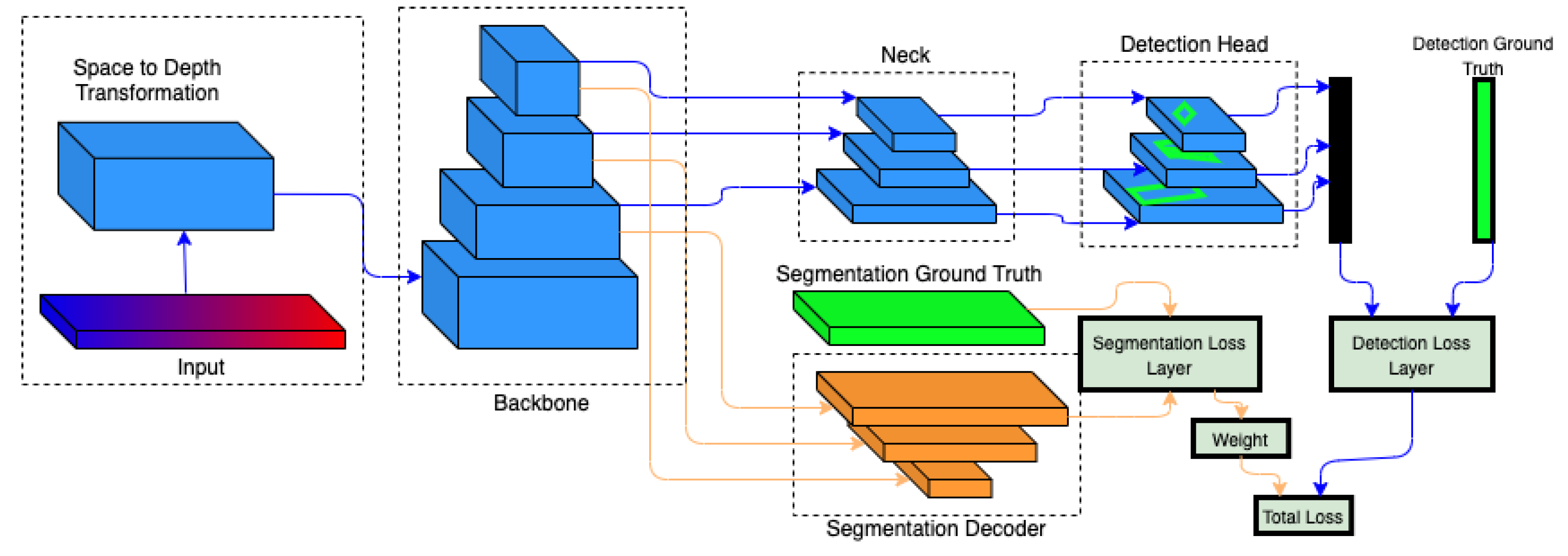
3.1.1. Vehicle Detection Architecture

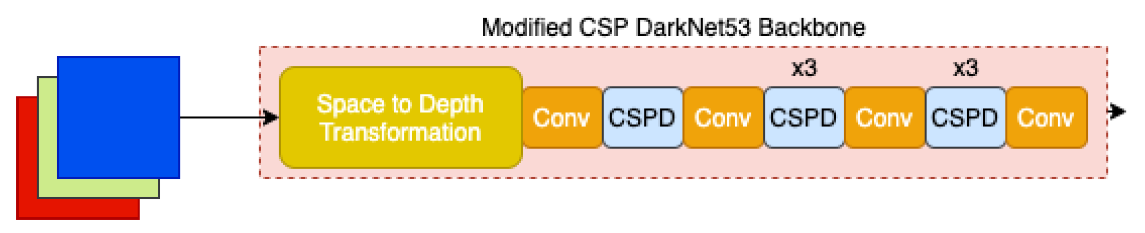
MulEYE’s multi-task vehicle detection architecture is composed of a backbone (where parameters are shared between the object detection and semantic segmentation tasks), the segmentation head, and the detection head. The complete architecture is shown in Figure 1. The design process started with finding a segmentation head that balanced computational speed and accuracy. Afterwards, an object detection task head was designed to provide maximum accuracy while still managing real-time performance. Finally, a backbone was chosen that as its main attribute improved vehicle detections, considering how this task was most important for the system goal.

Backbone

The CPSDarkNet53 was presented as one of the most important contributions of the YOLOv4 paper [28] due to the efficiency and processing boosted by Cross-stage partial connections (CSPs) inspired by CSPNet [73]. CSPs respected the variability of the gradients by integrating feature maps from the beginning and the end of a network stage, reducing computations by 20% without any detrimental effect on the accuracy.

However, the throughput of the original Darknet implementation of YOLOv4 on edge computational devices was low compared to the throughput on a GPU enabled desktop. Therefore, we modified the CPSDarkNet53 backbone architecture to make it shallower. In the proposed implementation, the number of CSP Bottleneck and Convolutional blocks was reduced and placed in an alternating way to optimize speed and accuracy of the standard and bottleneck layers [74]. This resulted in a lighter backbone version that was roughly 1/4th the size of the original: CSPDarkNet53 (Lite). More details on these blocks can be found in Bochkovskiy [28].

The reduced number of bottleneck layers increased the size of the latent space. This could affect the detection process, limiting the efficency in the encoding of features. This issue was ameliorated by adding a Space-to-Depth layer [74] to transform the input image to a lower spatial dimension while increasing the depth, to be fed into the light backbone. This module was inspired by the input procedure described in Ridnik [74] where this transformation efficiently reduced the input dimensions at the initial layers and improved the GPU inference throughput. The Space-to-depth layer transformed data from the form $[b,h,w,c]$ to $[b,h/2,w/2,4c]$, where b is the batch size, h is the height of the images, w is width, and c is the number of channels of the image. This was followed by a simple $1\times 1$ convolutional layer to match the channel depth of the network. In Ridnik [74], this transformation resulted in a 0.1% increase in accuracy and 4.2% increase in computational speed.

Figure 2 shows the schematic architecture of the CSPDarknet53(Lite) backbone, while details on the architecture can be found in

Table 1. The architecture of the CSPDarknet53(Lite) backbone with an added space-to-depth layer. CSP = cross-stage partial connection (CSP).

Name	Times Repeated	Filter Size
Input	1	-
Space-to-Depth	1	64
Conv	1	128
BottleneckCSP	1	128
Conv	1	256
BottleneckCSP	3	256
Conv	1	512
BottleneckCSP	3	512
Conv	1	1024

.

Semantic Segmentation Head

ENet [29] was chosen for the segmentation head because of its lightweight decoder. The original ENet was modified to adapt the expanded latent space due to the atrous convolutions used by the original ENet backbone. The decoder required additional layers in order to efficiently scale up the features. Skip-connections from the backbone were used to capture smaller scale features from the initial layers. These modifications resulted in a modified ENet, as summarized in

Table 2. The architecture of the modified ENet for semantic segmentation. Two additional bottleneck modules were introduced in stage 4 of the decoder, along with 3 skip-connections from the encoder. The additional modules are highlighted in blue.

Name	Type	Output Size
CSPDarkNet53 (Lite)	Backbone/Encoder	$16\times 16\times 576$
bottleneck4.0	upsampling	$32\times 32\times 256$
Concatenate	skip-connection from backbone	$32\times 32\times 544$
bottleneck4.1	upsampling	$64\times 64\times 128$
bottleneck4.2	upsampling	$128\times 128\times 64$
Concatenate	skip-connection from backbone	$128\times 128\times 136$
bottleneck4.3		$128\times 128\times 64$
bottleneck4.4		$128\times 128\times 64$
bottleneck5.0	upsampling	$256\times 256\times 16$
Concatenate	skip-connection from backbone	$256\times 256\times 32$
bottleneck5.1		$256\times 256\times 16$
Transposed Convolution		$512\times 512\times C$

. The main modifications made to the original ENet decoder architecture were:

• Two additional up-sampling bottleneck modules were implemented in the decoder (Table 2, bottlenecks 4.1 and 4.2) to compensate for the increase in the latent space dimensionality due to the lack of dilated convolutions in the CPSDarknet53 (Lite) backbone.
• Three skip-connections were implemented to link the backbone to the outputs of bottlenecks 4.0, 4.2, and 5.0, respectively, and to ease the learning of smaller scale features, similar as to the ones used in UNet [39].

Vehicle Detection Head

The vehicle detection head of the multi-task network was retained from the neck and head of the YOLOv4 [28] architecture without any modifications. The complete detection head consists of two parts: the YOLOv4 neck and the YOLOv3 head. The neck consists of the Path-Aggregation Network (PANet) [75] and the Spatial Pyramid Pooling (SPP) [76] modules. The function of the neck is to combine features of various scales that are generated in the different levels of the backbone. This is done by attaching an SPP module to the backbone in order to increase the receptive field and to choose the most important features from the backbone. These features are then aggregated by a PANet module.

The YOLO head, similar as to the one used by YOLOv3 [21], generated detections from the multi-level aggregated features generated by PANet. The PANet generated features of size 13 × 13, 26 × 26, and 52 × 52. The head divided these features into a grid of 9 cells each. Anchor boxes were then assigned to each grid cell in each level. Nine different anchor boxes were defined, each with its own aspect ratio with each feature level being assigned three anchor boxes. The anchor boxes that were closest to the ground truth were retained and the rest were discarded during inference by a process called non-maximum suppression.

Vehicle Detection Loss

MultEYE’s vehicle detection architecture was trained by combining the losses of each individual task. Unlike the loss calculation of single-task networks, the loss was calculated as additional layers: the segmentation loss and the detection loss layers. The losses of each task were combined and the architecture’ output was a combined loss, which was minimized during the training. The architecture accepted the training image as the input while the detection ground truth and the corresponding segmentation ground truth were passed to the network to calculate the corresponding losses. The strength of this architecture lies in the fact that the ground truth and loss layers were stripped from the architecture during inference (Figure 1). In this way, the size of the vehicle detection architecture was reduced significantly and, therefore, optimized for deployment on an edge-computing device.

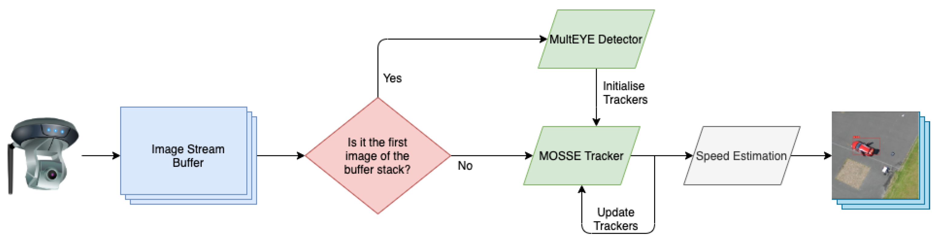
3.1.2. Vehicle Tracking—Minimum Output Sum of Squared Error (MOSSE)

The detections from the MultEYE vehicle detection network are used to initialize the object tracking algorithm. The Minimum Output Sum of Squared Error (MOSSE) algorithm was used for object tracking because of its ability to estimate the location of the tracked object at high computational speeds and accuracies using correlation filters [69]. MOSSE used the first two frames to initialize. The area enclosed by the bounding box of a detection was cropped from the first frame of the sequence and subsequently used as the template for initialization. This template was first transformed using a natural logarithmic transformation to reduce lighting effects and for contrast enhancement. Next, the template was expressed in its frequency domain by finding its Discrete Fourier Transform (DFT). Once the DFT was generated, a synthetic target was generated to be used in the initialization of the tracker and for updating the filter during tracking. This synthetic target contained a Gaussian peak centered at the object in the template (see Figure 3). With the Fourier transform and the synthetic target extracted, the MOSSE filter was initialized using the following formula [69]:

$$H^{*}=\frac{{\sum }_i{G}_i\odot F_i^{*}}{{\sum }_i{F}_i\odot F_i^{*}+ϵ},$$

(1)

where $H^{*}$ is the complex conjugate of the filter; $F_i$ and $G_i$ are the fourier transform and the synthetically generated target of the template in the $ith$ frame, respectively; and $F_i^{*}$ is the complex conjugate of $F_i$. The symbol ⊙ denotes an element-wise multiplication. Once the filter was initialized, the tracking filters could be estimated using the following formula [69]:

$$\begin{gathered} N_i=\eta \left(G_i,\odot ,F_i^{*}\right)+(1-\eta )N_{i-1} \\ {D}_i=\eta \left(F_i,\odot ,F_i^{*},+,ϵ\right)+(1-\eta )D_{i-1}. \\ {H}_i^{*}=\frac{D_i}{N_i} \end{gathered}$$

(2)

The term $\eta$ represents the learning rate, which ranges from 0 to 1. Once $H_i^{*}$ (the MOSSE filter of $ith$ frame) was determined, the position of the new object was determined by element-wise multiplication of the MOSSE filter with the cropped and transformed tracking window (Equation (3)).

$$G=H^{*}\odot F.$$

(3)

The tracking performance was further boosted by using a higher number of training samples or initialization frames. This was achieved by increasing the number of initialization frames by applying for example other transformations to the image in addition to the normalization and logarithmic transformation [69]. In this case, scale, translation and rotation transformation were performed using the following equations.

$$\left[\begin{array}{c}u\hfill \\ v\hfill \\ 1\hfill \end{array}\right]=\left[\begin{array}{ccc}1\hfill & 0\hfill & t_x\hfill \\ 0\hfill & 1\hfill & t_y\hfill \\ 0\hfill & 0\hfill & 1\hfill \end{array}\right]\left[\begin{array}{ccc}cos\left(\theta \right)\hfill & -sin\left(\theta \right)\hfill & 0\hfill \\ sin\left(\theta \right)\hfill & cos\left(\theta \right)\hfill & 0\hfill \\ 0\hfill & 0\hfill & 1\hfill \end{array}\right]\left[\begin{array}{ccc}1\hfill & 0\hfill & -t_x\hfill \\ 0\hfill & 1\hfill & -t_y\hfill \\ 0\hfill & 0\hfill & 1\hfill \end{array}\right],\left[\begin{array}{c}x\hfill \\ y\hfill \\ 0\hfill \end{array}\right]$$

(4)

$$\left[\begin{array}{c}u\hfill \\ v\hfill \\ 1\hfill \end{array}\right]=\left[\begin{array}{ccc}1\hfill & 0\hfill & t_x\hfill \\ 0\hfill & 1\hfill & t_y\hfill \\ 0\hfill & 0\hfill & 1\hfill \end{array}\right]\left[\begin{array}{ccc}s\hfill & 0\hfill & 0\hfill \\ 0\hfill & s\hfill & 0\hfill \\ 0\hfill & 0\hfill & 1\hfill \end{array}\right]\left[\begin{array}{ccc}1\hfill & 0\hfill & -t_x\hfill \\ 0\hfill & 1\hfill & -t_y\hfill \\ 0\hfill & 0\hfill & 1\hfill \end{array}\right]\left[\begin{array}{c}x\hfill \\ y\hfill \\ 0\hfill \end{array}\right],$$

(5)

where u and v are the coordinates of the new pixel, and x and y that of the old pixel. The symbols $t_x$ and $t_y$ represents the distance of the center of the image from the x and y axis, respectively, while the rotation angle and the scale is represented by $\theta$ and s, respectively.

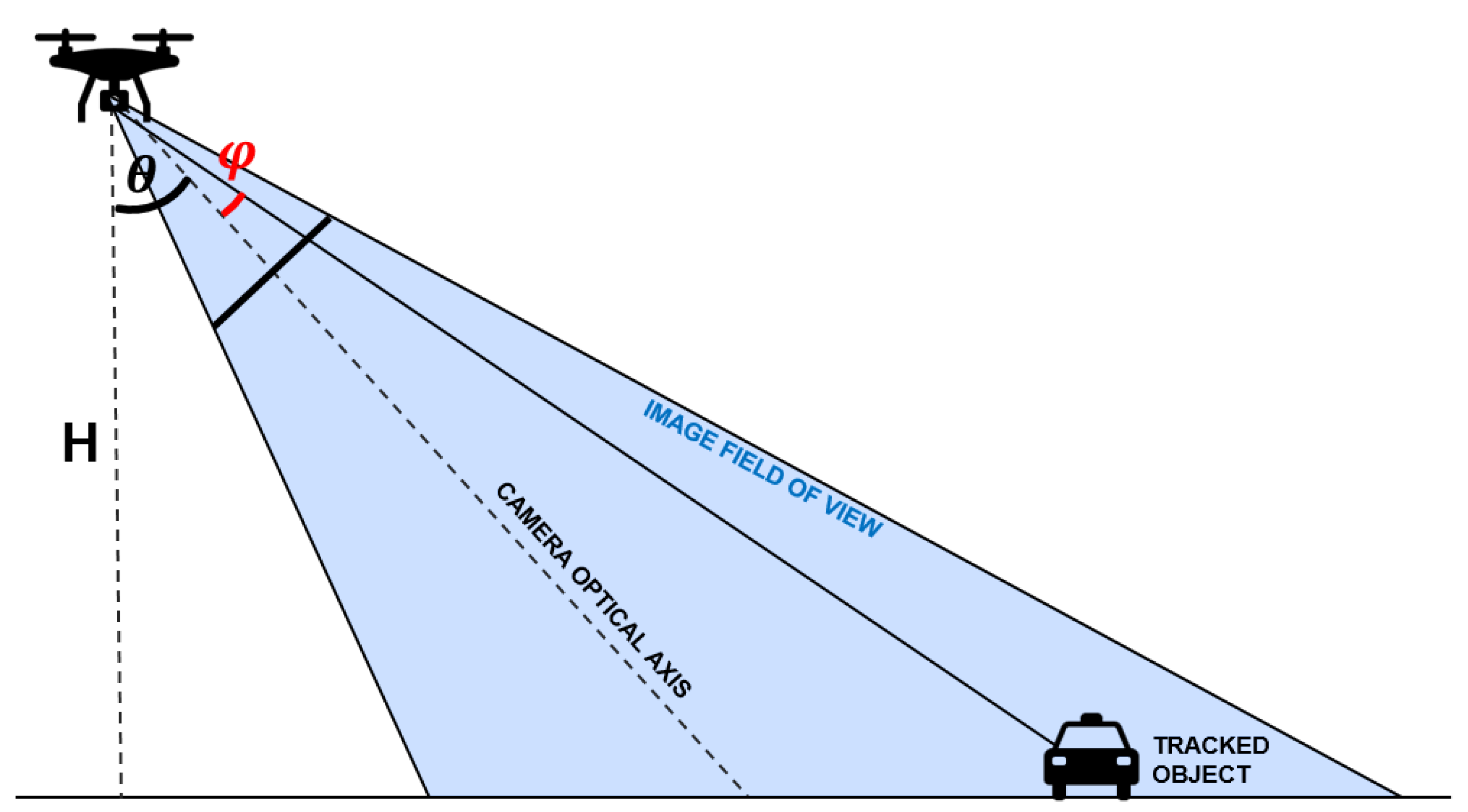
3.1.3. Speed Estimation

Tracking was important for vehicle speed estimation because the tracker preserved the identity of the object through two or more frames. Although the relative displacement of the object in two consecutive frames could be estimated easily, its transformation into the object space (i.e., world coordinate system) to estimate the object speed required additional steps, as well as the knowledge of two parameters: the Ground Sampling Distance (GSD) and the UAV’s velocity vector. The GSD corresponds to the size of a single pixel in the object space. For nadir views, the GSD can be considered constant throughout the image, whereas, for an oblique view, the GSD changes more significantly across the image. The calculation of the GSD on-board an UAV requires intrinsic camera parameters (see Equation (6)), as well as basic flight information (such as altitude, position, and camera angle), which could be retrieved by the on-board processing unit from the autopilot. Figure 4 depicts a scheme of the parameters involved in the GSD for oblique views.

In particular, the GSD for a nadir image could be estimated as follows:

$$GSD=\frac{H\times S_w}{F},$$

(6)

where H is the flight altitude in meters, $S_w$ is width of the pixel in the camera sensor, and F is the focal length. For oblique images, the nadir GSD could be used to calculate the corresponding oblique GSD at the certain tilt angle by multiplying this value by the GSD Rate as described in Equation (7):

$$GS{D}_{Rate}=\frac{1}{cos(\theta +\varphi )},$$

(7)

where $\theta$ is the camera tilt (referred to the optical axis). $\varphi$ describes the angular position of the pixel in the image: it is zero in correspondence of the optical axis of the camera, while it can have positive or negative values for the other pixels, as shown in Figure 4.

Assuming that the UAV and the tracked object are flown in a parallel trajectory, which is usually a good approximation for road monitoring, the speed of the detected vehicle could be formulated in the following way:

$$V=\frac{|{\overrightarrow{D}}_{UAV}-({\overrightarrow{D}}_{box}\times GSD\times GS{D}_{Rate})|}{f},$$

(8)

where ${\overrightarrow{D}}_{box}$ defines the displacement in pixels of the tracked object, while ${\overrightarrow{D}}_{UAV}$ (expressed in meters) is given by the position difference of the UAV retrieved from the on-board GNSS in a certain f interval.

3.2. Data

Given the aims of our work, available datasets should fulfil the following requirements:

• Altitude: images needed to be captured between 20 m and 150 m flight height to mimic UAV acquisitions [77].
• Number of Classes: the higher the number of classes, the greater the contextual awareness the object detector could learn. A minimum of five annotated classes was, therefore, needed. This eliminated datasets with only segmented road and/or buildings.
• Viewing Angle: to ensure drivers safety, UAV’s are currently not allowed to fly directly over the road but only alongside roads [77]. This essentially rendered all orthographic-only image datasets unusable to our application. Only images depicting the scene in a rough isometric view would be used.

These constraints depleted an already scarce pool of candidate datasets, reducing it to few multi-class segmentation datasets. For object detection, we used the Aeroscapes dataset [78] and collected additional UAV data of vehicles using a fixed wing UAV for further testing purposes. Vehicle tracking and speed estimation were assessed using the Karlsruhe Institute for Technology Aerial Image Sequences (KIT AIS) dataset [79]. Additional UAV data of bike riders, used as a proxy for vehicles, were collected to have ground-truth values. These datasets are further described below.

3.2.1. Vehicle Detection and Segmentation Dataset

The Aeroscapes dataset is an aerial semantic segmentation benchmark dataset that was collected using a DJI Phantom 3 fleet of drones between the altitudes of 5 and 50 m [78]. The dataset consisted of 3269 720p non-sequential images and their respective 11 class annotations. The dataset was split in the ratio of 70:20:10 as training, validation and testing datasets resulting in 2288 training samples, 654 validation samples and 327 test samples, respectively. No dataset including both multi-class semantic segmentation and vehicle detection annotations was available. Therefore, the Aeroscapes dataset was annotated for instances of vehicle class to train the object detector using the existing multi-class segmentation pixel-wise annotations.

MultEYE was designed to be implemented on an UAV flying at a higher altitude range compared to the ones used to collect the Aeroscapes dataset. Moreover, the Aeroscapes scenes were often not representative for large-scale traffic monitoring tasks as it contained scenes of static (parked) cars or cars moving in a small infrastructure network. Therefore, an additional set of images was captured by a fixed-wing UAV equipped with a Sensefly SODA camera. These images were used to increase the size of the test dataset and to evaluate the efficacy of the model. This SODA dataset contained 52 images taken at 30, 60, and 120 m altitudes at 5472 × 3648 resolution to investigate the performance using different GSD. The images were manually annotated.

Both datasets were prepared for training by resizing, normalizing and encoding them. The Aeroscapes images were resized from the original size of 1280 × 720 pixels to 512 × 512 pixels to reduce computational effort during training. On the opposite end, the SODA dataset was processed using a sliding window to splice large images to smaller chunks, preserving the GSD. Finally, all the images were normalized and one-hot-encoded by applying a color mask to each of the colors corresponding to their respective class and extracting a binary image for each of the classes.

3.2.2. Vehicle Tracking and Speed Estimation Dataset

The multi-object tracking was trained on a custom dataset with 100 image sequences derived from the KIT AIS Dataset [79]. The image sequences were captured 0.33 s apart with an average of 14 targets to track throughout the 100 images. There was no movement of the camera frame and none of the targets in the image was occluded from the point of their appearance in the sequence and their eventual exit from the frame of observation. The vehicle initialization was manually annotated so that the potential errors caused by an object detector did not influence the performance evaluation of the tracker.

For the speed estimation task, it was decided to detect and track bicycles instead of cars to ease the data collection step. Cars would have required a larger area to cover by the UAV and to cordon-off roads, making this experiment unpractical. Bicycles provided an easy alternative to cars to prove the speed methodology without any change to the model architecture and hence throughput speed. The captured dataset comprises six videos gathered at two locations using a DJI Phantom 4 UAV. The videos show cyclists cycling their bikes at different speeds. To acquire these videos, 10 participants were asked to ride their bicycles on a pre-defined stretch of road at a constant speed of their choice while using an app-based speed tracker to help themselves maintain this chosen speed and to use this information as ground truth in the testing phase. While the participants performed the circuit, the UAV was flown parallel to the predefined route at different altitudes. The essential flight data, such as GPS location, altitude, and camera angle, were logged for each frame of the captured video. Each video was then sampled at five frames per second to generate six corresponding image sequences.

3.3. Experiments

3.3.1. Vehicle Detection

The training strategy used for the multi-task training was similar to the one employed for the standard object detection problems by first coarsely, and afterwards fine-tuning the backbone and the different segmentation heads. To train the architecture coarsely, the backbone was initialized with pre-trained ImageNet weights [80]. While freezing the initialized backbone, only the detection head and the segmentation decoder were trained for 20 epochs. This ensured that the gradients did not explode or output high losses. Afterwards the backbone was unfrozen and the complete network was fine-tuned using a batch size of 4 for 250 epochs. The Tversky Loss for segmentation, the Generalized Intersection over Union (gIoU), for vehicle location and the Focal loss for vehicle confidence were used in combination with an ADAM optimizer [20,81,82]. Training was done on a workstation with an Intel Xeon Processor and a 12 GB NVIDIA Titan Xp GPU.

The trained vehicle detection network was evaluated against the test set of Aeroscapes and the SODA dataset by calculating the mean Average Precision (mAP) at a threshold level of 50%, meaning that the predicted bounding box and the ground truth overlap at least for 50%. The network was compared with different state of the art models that claimed real-time, >20 frames per second (FPS), performance. As explained in Section 3.1.1, before the evaluation, the network was stripped off the segmentation layers in order to retain the speed of the object detector.

3.3.2. Vehicle Tracking and Speed Estimation

The MOSSE tracker was evaluated using the KIT AIS Dataset. In practice, the output bounding boxes generated by the object detector were used to initialize the multi-object tracker on the input image. However, the annotated dataset was used in the evaluation to ensure that the errors in detection did not affect the tracking results. Therefore, the dataset with the images and their bounding boxes were fed to a mixture of classical and state-of-the-art tracking algorithms. The generated object positions were then compared with the ground truth obtained from the dataset. The evaluation metrics used for the trackers are Multi-object Tracking Accuracy (MOTA), Multi-object Tracking Precision (MOTP) and the Average Framerate [83]. MOTA is calculated using the following formula:

$$MOTA=1-\frac{{\sum }_t\left(m_t,+,f,p_t,+,m,m,e_t\right)}{{\sum }_t{g}_t},$$

(9)

where $m_t,f{p}_t$, and $mm{e}_t$ are the number of initialization misses, false positives, and mismatches, respectively, of time t, while $g_t$ is the number of ground truth instances at time t.

The MOTP is given by:

$$MOTP=\frac{{\sum }_{i,t}{d}_{i,t}}{{\sum }_t{c}_t}.$$

(10)

This formula essentially describes the ratio of the cumulative sum of position errors to the total number of detections. The Average Framerate is calculated as the sum of processing rate in frames/second for 100 frames divided by 100.

The speed estimation methodology was investigated using the bicycle dataset. The bicycle detector was trained using the same steps described in Section 3.3.1, except now the annotations were done on bicycle pixels instead of cars. This resulted in an object detection model for bicycle detection. Afterwards, for each sequence of images, the speed of the visible cyclists was computed. Ideally, two tracked image frames were enough to make an estimation of the vehicle speed; however, the average of eight tracked frames was used to filter the errors induced by outliers, while assuming constant speed. Longer sub-sequences would not make sense from an application point of view as vehicles tend to have variable speeds through the sequence and new vehicles entering the frame could not be initialized by the detector. The speed estimations were evaluated against the ground truth by calculating the average error over the complete sequence.

3.3.3. Inference on Jetson Xavier NX

To gain insight into the practicality of the designed system, we benchmarked the whole inference pipeline on an edge-computing device. Specifically, we investigated (1) the detection inference speed at different power usage settings and image sizes, (2) the combined vehicle detection, tracking and speed estimation at different power usages and images sizes, and (3) the optimization of image streaming. The datasets used for these experiments consisted of the bicycle dataset as it had information for detection, tracking and speed estimation, all of which need to be benchmarked on the Jetson Xavier NX board.

We used NVIDIA’s Jetson Xavier NX to benchmark the performance of MultEYE. The Jetson Xavier NX has six central processing units (CPUs) cores and a GPU with 384 CUDA cores. The board runs in two power modes, 10- or 15-Watt mode, which affect the inference speed, too. The difference in power modes correspond to the difference in number of processes parallelized by the GPU. Maximum throughput is achieved using 15 W mode. Apart from the GPU, the board also has 6 CPU cores which can be used to parallelize other processes.

The vehicle detection architecture was designed to work on two CPU cores and all CUDA cores in order to perform at its best. First, we investigated how the inference speed of the vehicle detection architecture was affected when run at a 10- and 15-Watt mode using different image resolutions. The input image resolutions were set at 512 × 230, 1024 × 1152 and 3072 × 1728.

Algorithms that run on CPU rarely show any significant difference in performance speed across devices. However, it is very insightful to monitor the performances of CPU based algorithms for vehicle tracking and speed estimation combined with object detection algorithms (running on GPU) on the embedded platform. The inference time needed for these three tasks, together using different image resolutions, was investigated to identify potential bottlenecks.

An additional test on data streaming was then performed to optimize the frame-rate of processed images. The performances reported in the other tests were achieved under the assumption that each image must go through the complete pipeline. However, this is not strictly necessary when multiple images of the same sequence are streamed in real-time (Figure 5). In this case, only the first image of the stack can be processed by the MultEYE detector, which initializes the MOSSE tracker for each of the vehicles, while the other images in the sequence can be directly fed sequentially into the tracker algorithm to estimate the speed. In this test, it was assessed how this strategy affected the processed frame-rate using sequences of 10 images with 3072 × 1728 pixels resolution.

4. Results & Discussion

4.1. Vehicle Detection

From the performed tests, MultEYE’s object detector achieved higher mAP then other state-of-the-art methods, showing that an auxiliary task (segmentation) improved the performance of the main task (detection). In particular, the implemented network yielded higher mAP values, despite having a relatively low number of parameters at one of the best frame-rates. These findings are reflected in

Table 3. Comparison of the MultEYE’s object detection network with other state-of-the-art models evaluated on a combination of 10% set of Aeroscapes and SODA Dataset images resized at 512 × 512 (except the SSD network that was trained with 300 × 300 resolution). The evaluation was benchmarked on a single NVIDIA Titan Xp GPU.

Model	Backbone	[email protected]%	No. of Parameters (M)	FPS
MultEYE	CSPDarkNet53(Lite)	0.834	12.4	43.5
YOLOv4 [28]	CSPDarkNet53 (Lite)	0.8073	12.4	43.88
	CSPDarkNet53 [28]	0.8172	37.3	31.19
	EfficientNet(B1) [84]	0.824	58.6	22.72
	MobileNetV3 [85]	0.746	19.13	41.5
	MobileNetV3Small [85]	0.694	11.6	57.13
TinyYOLOv4 (Custom)	EfficientNet (B1) [84]	0.7082	27.42	37.2
	MobileNetV3 Small [85]	0.6733	5.41	110.11
YOLOv3 [86]	Xception [87]	0.7625	42.53	20.8
SSD [52] (300 × 300)	VGG16 [88]	0.7739	24.0	39
	MobileNetV3 [85]	0.7156	9.6	59.3
Faster RCNN [19]	VGG 16 [88]	0.7910	71.93	6.62

.

The influence of segmentation to learn features of the object of interest was further analyzed. Figure 6 depicts the activation in the first channel of one of the final convolutional layer output of the backbone. It could be observed that the single task backbone activation (Figure 6b) was noisier than the same learned with a multi-task methodology (Figure 6c), while multi-task seemed to be able to detect the presence of vehicles in a sharper way. This could be explained by the implicit data augmentation capability of the multi-task process that learned how to ignore the noise of the single tasks and generalized this learnt information in a robust and efficient manner.

This was especially evident in the results achieved with the SODA dataset, which was characterized by a larger variability in the image resolution due to different flight heights. The object detector was able to detect cars correctly at very low resolution. While YOLOv4 yielded a low IoU score of 0.132 (Figure 7a), MultEYE’s object detector yielded a much higher score (0.844) (Figure 7b). This difference could be attributed to the limited training dataset that caused the YOLOv4 to overfit on Aeroscapes. On the opposite end, overfitting was prevented in MultEYE’s object detector due to the introduction of inductive bias, which in turn helped its regularization.

4.2. Vehicle Tracking

Table 4. Comparison of commonly used trackers with established state-of-the-art deep learning based trackers on the customized KIT AIS dataset. The ${}^{*}$ denotes that the tracker algorithm is deep-learning based and the speed was evaluated on a GPU (NVIDIA Titan Xp).

	MOTA	MOTP	Avg.Framerate (FPS)
BOOSTING [89]	35.92	44.32	<1
Multiple Instance Learning [90]	60.4	64.0	<1
Kernalized Correlation Filters [92]	80.2	87.8	8.3
Tracking Learning and Detection [91]	78.34	82.3	<1
MEDIANFLOW [93]	94.73	63.14	6.6
GOTURN ${}^{*}$ [68]	67.5	75.2	20.0
CSRT [94]	95.0	94.3	1.3
MOSSE [69]	90.91	92.11	227.5
POI * [95]	96.83	97.71	11.2
DeepSORT ${}^{*}$ [64]	94.85	93.29	40.4

shows the comparison of MOSSE with other commonly used trackers when applied to the customized KIT AIS dataset. It can be seen that old algorithms, like BOOSTING [89], Multiple Instance Learning (MIL) [90], and Tracking Learning Detection (TLD) [91], performed poorly, with higher processing times. This was most likely due to difficulty of these algorithms to maintain tracker identity when implemented as a Multi-Object Tracker considering how these were designed to be a single object tracker. Only GOTURN [68], DeepSORT [64] and MOSSE [69] achieved a faster tracking speed than the ones showed by object detection algorithms.

Despite their performance, GOTURN and DeepSORT are deep learning based algorithms that credit their accuracy and speed to GPU based computing. They could interfere with other algorithms that use graphical units, such as MultEYE’s object detector. Therefore, their usage was not preferable. By contrast, MOSSE’s execution speed was higher, despite running on CPU, and still reached comparable MOTA and MOTP values with its competitors.

Finally, since large numbers of tracking target usually enter and leave the frame in a short amount of time during a surveillance mission, it was essential that the trackers were initialized frequently to purge the objects that have already left the frame and to introduce trackers of objects that have newly entered the frame. This update frequency was empirically determined to be once every 10 frames. This tracker update rate, however, showed that Person Of Interest (POI), DeepSORT, and MOSSE performed almost identically with respect to the tracking accuracy, further confirming that MOSSE was the best choice for our developed system.

4.3. Speed Estimation

The average errors between the ground truth and estimated speed in all frames were estimated for all the six bicycle sequences.

Table 5. Average errors in the speed estimation on the collected image sequences.

	Avg. Error (km/h)
Sequence 1	0.85
Sequence 2	1.03
Sequence 3	1.43
Sequence 4	0.71
Sequence 5	1.25
Sequence 6	1.52
Mean Avg. Error (km/h)	1.13

shows the average error for all recorded sequences of the bicycle dataset. In the first sequence (Sequence 1), both the camera and the target (bicycles) were stationary (Figure 8a). This sequence was used to benchmark the errors propagated to the speed measurements due to the inaccurate measurements delivered by the navigation unit of the used UAV and the approximations of the developed algorithm.

In all the other sequences, both UAV and targets were moving, resembling a realistic traffic scene (Figure 8b). For instance, in Sequence 5 the target was moving at 15 km/h while the UAV flew at 27 km/h in the opposite direction. The algorithm predicted an average target speed of 16.25 km/h with an error lower than 1.5 km/h.

Although the speed range in our experiments was relatively small (maximum speed 30 km/h), the speed estimates had minimal variance with a negligible but constant offset from the ground truth. This could be attributed to errors in the on-board instrumentation or approximations adopted in the algorithm. Despite the offset, across all the 6 sequences, the mean baseline compensated average error was 1.13 km/h, which is lower than the average error found for common traffic speed cameras (3.2 km/h) [96].

4.4. Inference on Jetson Xavier NX

The main difference between different computing platforms is their compute capability. Therefore, the evaluation of the system pipeline on the edge computing device was based on the computational speed of the pipeline at different image input sizes, quantified by the frames processed per second (FPS).

4.4.1. Vehicle Detection Inference

Figure 9 shows the inference speed achieved by MultEYE’s object detection model for different input image resolutions ran at 10 and 15 W modes, respectively. It could be observed that the model achieved a real-time performance of 29.41 FPS for input resolution 512 × 320 running in 15 W power mode. When the image resolution was increased, the FPS decreases, as expected. However, the difference of FPS between the two power modes decreases, making less inconvenient to use 10 W for processing images of 2048 × 1152 pixel size and above.

4.4.2. Complete Pipeline Inference

Table 6. Percentage contribution of each algorithm in the pipeline towards the total runtime for four different resolutions.

Resolution	% Contribution of Detection	% Contribution of Tracking	% Contribution of Speed Estimation	Total Runtime (seconds)	FPS
512 × 320	88.54	11.45	∼0	0.0384	26.04
1024 × 576	93.74	6.25	∼0	0.0704	14.2
2048 × 1152	96.8	3.2	∼0	0.1364	7.33
3072 × 1728	98.36	1.64	∼0	0.2674	3.74

shows the contribution of the different elements composing the proposed system in terms of processing time. These results considered that each algorithm (i.e., detection, tracking and speed estimation) is ran for every image frame to estimate the total run-time of the pipeline on the Xavier NX board.

The processing speed ranged from 26 FPS with low resolutions to almost 4 FPS with higher resolutions. The speed estimation had negligible processing times compared to the other algorithms as it ran in less than ${10}^{-5}$ s. This could be explained by its simple implementation, involving only algebraic and trigonometric calculations, which are highly optimized in all the programming languages.

The detection algorithm contributed the most to the total run-time because neural networks are more computationally intensive than simpler tracking algorithms, even when ran on GPU. This was further exacerbated when using higher image resolutions: in this case, the detection took up a higher percentage of the total run-time, while the tracking algorithm faced only small changes because its speed only depended on the size of the object tracked. These findings entail that, though detection dictates major part of the frame-rate, a near-constant processing time for the tracking enables us to use higher number of tracking frames to improve the overall speed of the system.

4.4.3. Streaming Optimization

Complementing the results presented in the previous section, we now turn to streaming optimization. A buffer of 10 images was streamed into the pipeline, while running the detection algorithm only on the first frame and the tracking algorithm sequentially on all 10 images. As shown in

Table 7. Average frame rates for the pipeline for a sample stream buffer size of 10 images for four different resolutions.

Resolution	Average FPS
512 × 320	142.85
1024 × 576	98.03
2048 × 1152	59.52
3072 × 1728	33.04

, different image resolutions were considered. It was noticed that the FPS values were much higher than in Section 4.4.2, showing a significant boost when the pipeline was processed in this way. For instance, analyzing the contribution of each algorithm for the highest image resolution, the detector took 0.263 s to process the first frame while the rest of the 9 frames were processed by the tracking and speed estimation algorithms at a rate of 0.0044 (seconds/frame). As a result, the complete algorithm took

$$0.263+(0.0044\times 9)=0.3026\left(\sec \mathrm{onds}\right)$$

to process the entire buffer, which put the average run-time per image at 0.03026 seconds per image or 33.04 FPS.

It must be noticed that the images were streamed from a video file stored on the disk at 30 FPS, taking care to simulate perfectly an aerial camera platform streaming images, velocity and altitude parameters to the Xavier NX. However, possible delays due to asynchronous data stream of flight parameters and the images were not considered in this experiment.

5. Conclusions

This paper presented MultEYE, a traffic monitoring system that can detect, track, and estimate the velocity of vehicles in a sequence of aerial images. The system has been optimized such that it can be executed in real-time on an embedded computer mounted on an UAV. Although it is still in its developing phase, the system is to the best of authors’ knowledge, one of the first traffic monitoring systems specifically designed and optimized for an UAV platform.

In order to overcome the limitation of existing architectures related to accuracy and computational overhead, a multi-task learning methodology was employed by adding a segmentation head to the object detector backbone. The backbone and the segmentation head were optimized for vehicle detection. Learning the contextual features along with the detections showed to help the backbone of the network to better encode the features, especially the lower scale features. The number of bottlenecks in the backbone was reduced in order to generate a latent-space representation with fewer parameters, while additional bottlenecks and skip-connections were introduced in the segmentation head to be able to resolve the decoding of smaller-scale features in the images. Finally, the detection speed was preserved by detaching the segmentation head after training. The resulting vehicle detection model performed 4.8% better than the state-of-the-art algorithms for vehicle detection in aerial images, in terms of accuracy (mAP) while preserving the processing speed. Moreover, the vehicle detection network showed it is able to generalize to real world data, such as the used state-of-the-art dataset.

Besides vehicle detection, vehicle tracking and speed estimation were successfully executed on the edge-computing device at high inference speeds too. Vehicle tracking and speed estimation was achieved sequentially, after vehicles were detected by the neural network architecture. These algorithms were run on CPU in order to exploit all the computational resources of the on-board unit in an optimal way. The achieved results showed that the developed system can run in real-time using high-resolution images, too. Different strategies to increase the processed frame-rates were shown in the experiments.

MultEYE was developed under the most realistic conditions by testing the feasibility and pipeline of the system on an on-board computing device. Although the Aeroscapes dataset was adapted for the purpose of this work, only ∼20% of the images depicted vehicles. The additional datasets collected are still relatively limited to validate fully the proposed system in operational conditions. From this perspective, the acquisition of more realistic datasets over traffic scenes, capturing cars moving at high speed and in varying lighting conditions, could give a more complete insight on the performances of this system. Different flight heights could allow to furthering assessing the detection algorithm in different conditions. Then, the effectiveness of this solution could be verified with additional tests by running the developed system on an on-board unit flying on real traffic scenes.

Despite the existing limitations given by legislative restrictions and the still relatively limited battery endurance, the use of UAV for this or similar applications are expected to increase rapidly in the coming years. In this regard, the presented work represents a first meaningful step towards the development of efficient solutions for operational UAV traffic monitoring systems.

References

1. Gardner, M.P. Highway Traffic Monitoring; Technical Report; A2B08; Committee on Highway Traffic Monitoring Chairman; South Dakota Department of Transportation: Pierre, SD, USA, 2000. [Google Scholar]
2. Frank, H. Expanded Traffic-Cam System in Monroe County Will Cost PennDOT 4.3M. Available online: http://www.poconorecord.com/apps/pbcs.dll/articlAID=/20130401/NEWS/1010402/-1/NEWS (accessed on 27 July 2020).
3. Maimaitijiang, M.; Sagan, V.; Sidike, P.; Daloye, A.M.; Erkbol, H.; Fritschi, F.B. Crop Monitoring Using Satellite/UAV Data Fusion and Machine Learning. Remote Sens. 2020, 12, 1357. [Google Scholar] [CrossRef]
4. Raeva, P.L.; Šedina, J.; Dlesk, A. Monitoring of crop fields using multispectral and thermal imagery from UAV. Eur. J. Remote Sens. 2019, 52, 192–201. [Google Scholar] [CrossRef] [Green Version]
5. Feng, X.; Li, P. A Tree Species Mapping Method from UAV Images over Urban Area Using Similarity in Tree-Crown Object Histograms. Remote Sens. 2019, 11, 1982. [Google Scholar] [CrossRef] [Green Version]
6. Wu, X.; Shen, X.; Cao, L.; Wang, G.; Cao, F. Assessment of individual tree detection and canopy cover estimation using unmanned aerial vehicle based light detection and ranging (UAV-LiDAR) data in planted forests. Remote Sens. 2019, 11, 908. [Google Scholar] [CrossRef] [Green Version]
7. Noor, N.M.; Abdullah, A.; Hashim, M. Remote sensing UAV/drones and its applications for urban areas: A review. IOP Conf. Ser. Earth Environ. Sci. 2018, 169, 012003. [Google Scholar] [CrossRef]
8. Nex, F.; Duarte, D.; Tonolo, F.G.; Kerle, N. Structural Building Damage Detection with Deep Learning: Assessment of a State-of-the-Art CNN in Operational Conditions. Remote Sens. 2019, 11, 2765. [Google Scholar] [CrossRef] [Green Version]
9. Zhang, C.; Elaksher, A. An Unmanned Aerial Vehicle-Based Imaging System for 3D Measurement of Unpaved Road Surface Distresses. Comput. Aided Civ. Infrastruct. Eng. 2012, 27, 118–129. [Google Scholar] [CrossRef]
10. Tan, Y.; Li, Y. UAV Photogrammetry-Based 3D Road Distress Detection. ISPRS Int. J. GeoInf. 2019, 8, 409. [Google Scholar] [CrossRef] [Green Version]
11. Chen, S.; Laefer, D.F.; Mangina, E.; Zolanvari, S.M.I.; Byrne, J. UAV Bridge Inspection through Evaluated 3D Reconstructions. J. Bridge Eng. 2019, 24, 05019001. [Google Scholar] [CrossRef] [Green Version]
12. Elloumi, M.; Dhaou, R.; Escrig, B.; Idoudi, H.; Saidane, L.A.; Fer, A. Traffic Monitoring on City Roads Using UAVs. In Proceedings of the 18th International Conference on Ad-Hoc Networks and Wireless, ADHOC-NOW, Luxembourg, 1–3 October 2019; Springer International Publishing: Basel, Switzerland, 2019; pp. 588–600. [Google Scholar]
13. Stöcker, C.; Bennett, R.; Nex, F.; Gerke, M.; Zevenbergen, J. Review of the Current State of UAV Regulations. Remote Sens. 2017, 9, 459. [Google Scholar] [CrossRef] [Green Version]
14. Press. Dutch Government Successfully Uses Aerialtronics Drones to Control Traffic. Available online: https://www.suasnews.com/2015/07/dutch-government-successfully-uses-aerialtronics-drones-to-control-traffic/ (accessed on 27 July 2020).
15. Elloumi, M.; Dhaou, R.; Escrig, B.; Idoudi, H.; Saidane, L.A. Monitoring road traffic with a UAV-based system. In Proceedings of the IEEE Wireless Communications and Networking Conference (WCNC), Barcelona, Spain, 15–18 April 2018; IEEE: Piscataway, NJ, USA, 2018; pp. 1–6. [Google Scholar]
16. Khan, M.A.; Ectors, W.; Bellemans, T.; Janssens, D.; Wets, G. UAV-based traffic analysis: A universal guiding framework based on literature survey. Transp. Res. Procedia 2017, 22, 541–550. [Google Scholar] [CrossRef]
17. Niu, H.; Gonzalez-Prelcic, N.; Heath, R.W. A UAV-based traffic monitoring system—Invited paper. In Proceedings of the IEEE 87th Vehicular Technology Conference (VTC Spring), Porto, Portugal, 3–6 June 2018; IEEE: Piscataway, NJ, USA, 2018; pp. 1–5. [Google Scholar]
18. Kriegel, H.P.; Schubert, E.; Zimek, A. The (black) art of runtime evaluation: Are we comparing algorithms or implementations? Knowl. Inf. Syst. 2017, 52, 341–378. [Google Scholar] [CrossRef]
19. Ren, S.; He, K.; Girshick, R.; Sun, J. Faster R-CNN: Towards Real-Time Object Detection with Region Proposal Networks. IEEE Trans. Pattern Anal. Mach. Intell. 2017, 39, 1137–1149. [Google Scholar] [CrossRef] [Green Version]
20. Lin, T.Y.; Goyal, P.; Girshick, R.; He, K.; Dollár, P. Focal loss for dense object detection. In Proceedings of the IEEE International Conference on Computer Vision (ICCV), Venice, Italy, 22–29 October 2017; IEEE: Piscataway, NJ, USA, 2017; pp. 2999–3007. [Google Scholar]
21. Redmon, J.; Divvala, S.; Girshick, R.; Farhadi, A. You only look once: Unified, real-time object detection. In Proceedings of the IEEE Conference on Computer Vision and PATTERN Recognition, Venice, NV, USA, 27–30 June 2016; IEEE: Piscataway, NJ, USA, 2016; pp. 779–788. [Google Scholar]
22. Kwan, C.; Chou, B.; Yang, J.; Rangamani, A.; Tran, T.; Zhang, J.; Etienne-Cummings, R. Deep Learning-Based Target Tracking and Classification for Low Quality Videos Using Coded Aperture Camera. Sensors 2019, 19, 3702. [Google Scholar] [CrossRef] [PubMed] [Green Version]
23. Li, J.; Dai, Y.; Li, C.; Shu, J.; Li, D.; Yang, T.; Lu, Z. Visual Detail Augmented Mapping for Small Aerial Target Detection. Remote Sens. 2018, 11, 14. [Google Scholar] [CrossRef] [Green Version]
24. Caruana, R. Multitask learning. Mach. Learn. 1997, 28, 41–75. [Google Scholar] [CrossRef]
25. Hashimoto, K.; Xiong, C.; Tsuruoka, Y.; Socher, R. A joint many-task model: Growing a neural network for multiple nlp tasks. arXiv 2016, arXiv:1611.01587. [Google Scholar]
26. McCann, B.; Keskar, N.S.; Xiong, C.; Socher, R. The natural language decathlon: Multitask learning as question answering. arXiv 2018, arXiv:1806.08730. [Google Scholar]
27. Teichmann, M.; Weber, M.; Zöllner, M.; Cipolla, R.; Urtasun, R. MultiNet: Real-time Joint Semantic Reasoning for Autonomous Driving. In Proceedings of the IEEE Intelligent Vehicles Symposium (IV), Changshu, China, 26–30 June 2018; IEEE: Piscataway, NJ, USA, 2018; pp. 1013–1020. [Google Scholar]
28. Bochkovskiy, A.; Wang, C.Y.; Liao, H.Y.M. YOLOv4: Optimal Speed and Accuracy of Object Detection. arXiv 2020, arXiv:2004.10934. [Google Scholar]
29. Paszke, A.; Chaurasia, A.; Kim, S.; Culurciello, E. Enet: A deep neural network architecture for real-time semantic segmentation. arXiv 2016, arXiv:1606.02147. [Google Scholar]
30. Forsyth, D.A.; Ponce, J. Computer Vision: A Modern Approach; Prentice Hall: Upper Sadle River, NJ, USA, 2003; pp. 1–693. [Google Scholar]
31. Milletari, F.; Navab, N.; Ahmadi, S.A. V-net: Fully convolutional neural networks for volumetric medical image segmentation. In Proceedings of the 2016 Fourth International Conference on 3D Vision (3DV), Stanford, CA, USA, 25–28 October 2016; IEEE: Piscataway, NJ, USA, 2016; pp. 565–571. [Google Scholar]
32. Kim, J.; Park, C. End-to-end ego lane estimation based on sequential transfer learning for self-driving cars. In Proceedings of the IEEE Conference on Computer Vision and Pattern Recognition Workshops (CVPRW), Honolulu, HI, USA, 21–26 July 2017; IEEE: Piscataway, NJ, USA, 2017; pp. 1194–1202. [Google Scholar]
33. Ullah, M.; Mohammed, A.; Alaya Cheikh, F. Pednet: A spatio-temporal deep convolutional neural network for pedestrian segmentation. J. Imaging 2018, 4, 107. [Google Scholar] [CrossRef] [Green Version]
34. Ammar, S.; Bouwmans, T.; Zaghden, N.; Neji, M. Moving objects segmentation based on deepsphere in video surveillance. In Proceedings of the 14th International Symposium on Visual Computing, ISVC 2019, Lake Tahoe, NV, USA, 7–9 October 2019; Springer: Basel, Switzerland, 2019. Part II. pp. 307–319. [Google Scholar]
35. Long, J.; Shelhamer, E.; Darrell, T. Fully convolutional networks for semantic segmentation. In Proceedings of the IEEE Conference on Computer Vision and Pattern Recognition (CVPR), Boston, MA, USA, 7–12 June 2015; IEEE: Piscataway, NJ, USA, 2015; pp. 3431–3440. [Google Scholar]
36. Everingham, M.; Van Gool, L.; Williams, C.K.; Winn, J.; Zisserman, A. The pascal visual object classes (voc) challenge. Int. J. Comput. Vis. 2010, 88, 303–338. [Google Scholar] [CrossRef] [Green Version]
37. Silberman, N.; Hoiem, D.; Kohli, P.; Fergus, R. Indoor segmentation and support inference from rgbd images. In Proceedings of the 12th European Conference on Computer Vision, Florence, Italy, 7–13 October 2012; Springer: Berlin/Heidelberg, Germany, 2012. Part V. pp. 746–760. [Google Scholar]
38. Badrinarayanan, V.; Kendall, A.; Cipolla, R. Segnet: A deep convolutional encoder-decoder architecture for image segmentation. IEEE Trans. Pattern Anal. Mach. Intell. 2017, 39, 2481–2495. [Google Scholar] [CrossRef] [PubMed]
39. Ronneberger, O.; Fischer, P.; Brox, T. U-net: Convolutional networks for biomedical image segmentation. In Proceedings of the 18th International Conference, Munich, Germany, 5–9 October 2015; Springer: Basel, Switzerland, 2015. Part III. pp. 234–241. [Google Scholar]
40. Lin, G.; Milan, A.; Shen, C.; Reid, I. Refinenet: Multi-path refinement networks for high-resolution semantic segmentation. In Proceedings of the IEEE Conference on Computer Vision and Pattern Recognition (CVPR), Honolulu, HI, USA, 21–26 July 2017; IEEE: Piscataway, NJ, USA, 2017; pp. 5168–5177. [Google Scholar]
41. Chen, L.C.; Papandreou, G.; Schroff, F.; Adam, H. Rethinking atrous convolution for semantic image segmentation. arXiv 2017, arXiv:1706.05587. [Google Scholar]
42. Chen, L.C.; Papandreou, G.; Kokkinos, I.; Murphy, K.; Yuille, A.L. Deeplab: Semantic image segmentation with deep convolutional nets, atrous convolution, and fully connected crfs. IEEE Trans. Pattern Anal. Mach. Intell. 2017, 40, 834–848. [Google Scholar] [CrossRef] [PubMed]
43. Yu, F.; Koltun, V. Multi-scale context aggregation by dilated convolutions. arXiv 2015, arXiv:1511.07122. [Google Scholar]
44. Wang, P.; Chen, P.; Yuan, Y.; Liu, D.; Huang, Z.; Hou, X.; Cottrell, G. Understanding convolution for semantic segmentation. In Proceedings of the IEEE Winter Conference on Applications of Computer Vision (WACV), Lake Tahoe, NV, USA, 12–15 March 2018; IEEE: Piscataway, NJ, USA, 2018; pp. 1451–1460. [Google Scholar]
45. Yang, M.; Yu, K.; Zhang, C.; Li, Z.; Yang, K. Denseaspp for semantic segmentation in street scenes. In Proceedings of the IEEE/CVF Conference on Computer Vision and Pattern Recognition, Salt Lake City, UT, USA, 18–23 June 2018; IEEE: Piscataway, NJ, USA, 2018; pp. 3684–3692. [Google Scholar]
46. Girshick, R.; Donahue, J.; Darrell, T.; Malik, J. Rich feature hierarchies for accurate object detection and semantic segmentation. In Proceedings of the 2014 IEEE Conference on Computer Vision and Pattern Recognition, Columbus, OH, USA, 23–28 June 2014; IEEE: Piscataway, NJ, USA, 2014; pp. 580–587. [Google Scholar]
47. Girshick, R. Fast r-cnn. In Proceedings of the 2015 IEEE International Conference on Computer Vision (ICCV), Santiago, Chile, 7–13 December 2015; IEEE: Piscataway, NJ, USA, 2015; pp. 1440–1448. [Google Scholar]
48. Tan, M.; Pang, R.; Le, Q.V. Efficientdet: Scalable and efficient object detection. In Proceedings of the IEEE/CVF Conference on Computer Vision and Pattern Recognition (CVPR), Seattle, WA, USA, 13–19 June 2020; IEEE: Piscataway, NJ, USA, 2020; pp. 10778–10787. [Google Scholar]
49. Yang, M.Y.; Liao, W.; Li, X.; Cao, Y.; Rosenhahn, B. Vehicle detection in aerial images. Photogramm. Eng. Remote Sens. 2019, 85, 297–304. [Google Scholar] [CrossRef] [Green Version]
50. Sommer, L.W.; Schuchert, T.; Beyerer, J. Fast deep vehicle detection in aerial images. In Proceedings of the IEEE Winter Conference on Applications of Computer Vision (WACV), Santa Rosa, CA, USA, 24–31 March 2017; IEEE: Piscataway, NJ, USA, 2017; pp. 311–319. [Google Scholar]
51. Deng, Z.; Sun, H.; Zhou, S.; Zhao, J.; Zou, H. Toward fast and accurate vehicle detection in aerial images using coupled region-based convolutional neural networks. IEEE J. Sel. Top. Appl. Earth Obs. Remote Sens. 2017, 10, 3652–3664. [Google Scholar] [CrossRef]
52. Liu, W.; Anguelov, D.; Erhan, D.; Szegedy, C.; Reed, S.; Fu, C.Y.; Berg, A.C. SSD: Single shot multibox detector. In Proceedings of the 14th European Conference, Amsterdam, The Netherlands, 11–14 October 2016; Springer: Cham, Switzerland, 2016. Part I. pp. 21–37. [Google Scholar]
53. Olshausen, B.A.; Field, D.J. Emergence of simple-cell receptive field properties by learning a sparse code for natural images. Nature 1996, 381, 607–609. [Google Scholar] [CrossRef] [PubMed]
54. Bell, A.J.; Sejnowski, T.J. The “independent components” of natural scenes are edge filters. Vis. Res. 1997, 37, 3327–3338. [Google Scholar] [CrossRef] [Green Version]
55. Gidaris, S.; Komodakis, N. Object detection via a multi-region and semantic segmentation-aware cnn model. In Proceedings of the IEEE International Conference on Computer Vision (ICCV), Santiago, Chile, 7–13 December 2015; pp. 1134–1142. [Google Scholar]
56. Brahmbhatt, S.; Christensen, H.I.; Hays, J. StuffNet: Using ‘Stuff’to improve object detection. In Proceedings of the IEEE Winter Conference on Applications of Computer Vision (WACV), Los Alamitos, CA, USA, 24–31 March 2017; IEEE Computer Society: Piscataway, NJ, USA, 2017; pp. 934–943. [Google Scholar]
57. Shrivastava, A.; Gupta, A. Contextual priming and feedback for faster r-cnn. In Proceedings of the 14th European Conference, Amsterdam, The Netherlands, 11–14 October 2016; Springer: Cham, Switzerland, 2016. Part I. pp. 330–348. [Google Scholar]
58. He, K.; Gkioxari, G.; Dollár, P.; Girshick, R. Mask r-cnn. In Proceedings of the IEEE International Conference on Computer Vision (ICCV), Venice, Italy, 22–29 October 2017; pp. 2980–2988. [Google Scholar]
59. Lu, H.; Li, P.; Wang, D. Visual object tracking: A survey. Pattern Recognit. Artif. Intell. 2018, 31, 61–76. [Google Scholar]
60. Cuevas, E.; Zaldivar, D.; Rojas, R. Kalman Filter for Vision Tracking; Technical Report August; Freie Universitat Berlin: Berlin, Germany, 2005. [Google Scholar]
61. Okuma, K.; Taleghani, A.; De Freitas, N.; Little, J.J.; Lowe, D.G. A boosted particle filter: Multitarget detection and tracking. In Proceedings of the 8th European Conference on Computer Vision, Prague, Czech Republic, 11–14 May 2004; Springer: Berlin/Heidelberg, Germany, 2004. Part I. pp. 28–39. [Google Scholar]
62. Bochinski, E.; Eiselein, V.; Sikora, T. High-speed tracking-by-detection without using image information. In Proceedings of the 14th IEEE International Conference on Advanced Video and Signal Based Surveillance (AVSS), Lecce, Italy, 29 August–1 September 2017; IEEE: Piscataway, NJ, USA, 2017; pp. 1–6. [Google Scholar]
63. Bewley, A.; Ge, Z.; Ott, L.; Ramos, F.; Upcroft, B. Simple online and realtime tracking. In Proceedings of the IEEE International Conference on Image Processing (ICIP), Phoenix, AZ, USA, 25–28 September 2016; IEEE: Piscataway, NJ, USA, 2016; pp. 3464–3468. [Google Scholar]
64. Wojke, N.; Bewley, A.; Paulus, D. Simple online and realtime tracking with a deep association metric. In Proceedings of the IEEE International Conference on Image Processing (ICIP), Beijing, China, 17–20 September 2017; IEEE: Piscataway, NJ, USA, 2017; pp. 3645–3649. [Google Scholar]
65. Sadeghian, A.; Alahi, A.; Savarese, S. Tracking the untrackable: Learning to track multiple cues with long-term dependencies. In Proceedings of the IEEE International Conference on Computer Vision (ICCV), Venice, Italy, 22–29 October 2017; IEEE: Piscataway, NJ, USA, 2017; pp. 300–311. [Google Scholar]
66. Kart, U.; Lukezic, A.; Kristan, M.; Kamarainen, J.K.; Matas, J. Object tracking by reconstruction with view-specific discriminative correlation filters. In Proceedings of the IEEE/CVF Conference on Computer Vision and Pattern Recognition (CVPR), Long Beach, CA, USA, 15–20 June 2019; IEEE: Piscataway, NJ, USA, 2019; pp. 1339–1348. [Google Scholar]
67. Nam, H.; Han, B. Learning Multi-Domain Convolutional Neural Networks for Visual Tracking. In Proceedings of the IEEE Conference on Computer Vision and Pattern Recognition (CVPR), Las Vegas, NV, USA, 27–30 June 2016; IEEE: Piscataway, NJ, USA, 2016; pp. 4293–4302. [Google Scholar]
68. Held, D.; Thrun, S.; Savarese, S. Learning to track at 100 fps with deep regression networks. In Proceedings of the 14th European Conference on Computer Vision, Amsterdam, The Netherlands, 11–14 October 2016; Springer: Cham, Switzerland, 2016; pp. 749–765. [Google Scholar]
69. Bolme, D.S.; Beveridge, J.R.; Draper, B.A.; Lui, Y.M. Visual object tracking using adaptive correlation filters. In Proceedings of the IEEE Computer Society Conference on Computer Vision and PATTERN Recognition, San Francisco, CA, USA, 13–18 June 2010; IEEE: Piscataway, NJ, USA, 2010; pp. 2544–2550. [Google Scholar]
70. Schoepflin, T.N.; Dailey, D.J. Dynamic camera calibration of roadside traffic management cameras for vehicle speed estimation. IEEE Trans. Intell. Transp. Syst. 2003, 4, 90–98. [Google Scholar] [CrossRef]
71. Zhiwei, H.; Yuanyuan, L.; Xueyi, Y. Models of vehicle speeds measurement with a single camera. In Proceedings of the International Conference on Computational Intelligence and Security Workshops (CISW 2007), Harbin, China, 15–19 December 2007; IEEE: Piscataway, NJ, USA, 2007; pp. 283–286. [Google Scholar]
72. Li, J.; Chen, S.; Zhang, F.; Li, E.; Yang, T.; Lu, Z. An adaptive framework for multi-vehicle ground speed estimation in airborne videos. Remote Sens. 2019, 11, 1241. [Google Scholar] [CrossRef] [Green Version]
73. Wang, C.Y.; Mark Liao, H.Y.; Wu, Y.H.; Chen, P.Y.; Hsieh, J.W.; Yeh, I.H. CSPNet: A new backbone that can enhance learning capability of CNN. In Proceedings of the IEEE/CVF Conference on Computer Vision and Pattern Recognition Workshops (CVPRW), Seattle, WA, USA, 14–19 June 2020; IEEE: Piscataway, NJ, USA, 2020; pp. 1571–1580. [Google Scholar]
74. Ridnik, T.; Lawen, H.; Noy, A.; Friedman, I. TResNet: High Performance GPU-Dedicated Architecture. arXiv 2020, arXiv:2003.13630. [Google Scholar]
75. Liu, S.; Qi, L.; Qin, H.; Shi, J.; Jia, J. Path aggregation network for instance segmentation. In Proceedings of the IEEE Conference on Computer Vision and Pattern Recognition, Salt Lake City, UT, USA, 18–23 June 2018; IEEE: Piscataway, NJ, USA, 2018; pp. 8759–8768. [Google Scholar]
76. He, K.; Zhang, X.; Ren, S.; Sun, J. Spatial pyramid pooling in deep convolutional networks for visual recognition. IEEE Trans. Pattern Anal. Mach. Intell. 2015, 37, 1904–1916. [Google Scholar] [CrossRef] [PubMed] [Green Version]
77. Schultz van Haegen, M. Model Flying Scheme. Available online: https://wetten.overheid.nl/BWBR0019147/2019-04-01 (accessed on 22 July 2020).
78. Nigam, I.; Huang, C.; Ramanan, D. Ensemble knowledge transfer for semantic segmentation. In Proceedings of the IEEE Winter Conference on Applications of Computer Vision (WACV), Lake Tahoe, NV, USA, 12–15 March 2018; IEEE: Piscataway, NJ, USA, 2018; pp. 1499–1508. [Google Scholar]
79. Schmidt, F. Data Set for Tracking Vehicles in Aerial Image Sequences. Available online: http://www.ipf.kit.edu/downloads_data_set_AIS_vehicle_tracking.php (accessed on 22 July 2020).
80. Krizhevsky, A.; Sutskever, I.; Hinton, G.E. Imagenet classification with deep convolutional neural networks. In Proceedings of the Advances in Neural Information Processing Systems 25 (NIPS 2012), Lake Tahoe, NV, USA, 3–8 December 2012; pp. 1097–1105. [Google Scholar]
81. Salehi, S.S.M.; Erdogmus, D.; Gholipour, A. Tversky loss function for image segmentation using 3D fully convolutional deep networks. In Proceedings of the 8th International Workshop Machine Learning in Medical Imaging, Quebec City, QC, Canada, 10 September 2017; Springer International Publishing: Cham, Switzerland, 2017; pp. 379–387. [Google Scholar]
82. Rezatofighi, H.; Tsoi, N.; Gwak, J.; Sadeghian, A.; Reid, I.; Savarese, S. Generalized Intersection Over Union: A Metric and a Loss for Bounding Box Regression. In Proceedings of the IEEE/CVF Conference on Computer Vision and Pattern Recognition (CVPR), Long Beach, CA, USA, 15–20 June 2019; IEEE: Piscataway, NJ, USA, 2019; pp. 658–666. [Google Scholar]
83. Bernardin, K.; Elbs, A.; Stiefelhagen, R. Multiple object tracking performance metrics and evaluation in a smart room environment. In Proceedings of the The Sixth IEEE International Workshop on Visual Surveillance (in Conjunction with ECCV), Graz, Austria, 13 May 2006; Volume 90, p. 91. [Google Scholar]
84. Tan, M.; Le, Q.V. Efficientnet: Rethinking model scaling for convolutional neural networks. arXiv 2019, arXiv:1905.11946. [Google Scholar]
85. Howard, A.; Sandler, M.; Chen, B.; Wang, W.; Chen, L.; Tan, M.; Chu, G.; Vasudevan, V.; Zhu, Y.; Pang, R.; et al. Searching for mobilenetv3. In Proceedings of the IEEE/CVF International Conference on Computer Vision (ICCV), Seoul, Korea, 27 Octomber–2 November 2019; IEEE: Piscataway, NJ, USA, 2019; pp. 1314–1324. [Google Scholar]
86. Redmon, J.; Farhadi, A. Yolov3: An incremental improvement. arXiv 2018, arXiv:1804.02767. [Google Scholar]
87. Chollet, F. Xception: Deep learning with depthwise separable convolutions. In Proceedings of the IEEE Conference on Computer Vision and Pattern Recognition (CVPR), Honolulu, HI, USA, 21–26 July 2017; IEEE: Piscataway, NJ, USA, 2017; pp. 1800–1807. [Google Scholar]
88. Simonyan, K.; Zisserman, A. Very deep convolutional networks for large-scale image recognition. arXiv 2014, arXiv:1409.1556. [Google Scholar]
89. Grabner, H.; Grabner, M.; Bischof, H. Real-time tracking via on-line boosting. In Proceedings of the The British Machine Vision Conference, Edinburgh, Scotland, 4–7 September 2006; pp. 47–57. [Google Scholar]
90. Babenko, B.; Yang, M.H.; Belongie, S. Visual tracking with online multiple instance learning. In Proceedings of the IEEE Conference on Computer Vision and Pattern Recognition, Miami, FL, USA, 20–25 June 2009; IEEE: Piscataway, NJ, USA, 2009; pp. 983–990. [Google Scholar]
91. Kalal, Z.; Mikolajczyk, K.; Matas, J. Tracking-learning-detection. IEEE Trans. Pattern Anal. Mach. Intell. 2011, 34, 1409–1422. [Google Scholar] [CrossRef] [Green Version]
92. Henriques, J.F.; Caseiro, R.; Martins, P.; Batista, J. High-speed tracking with kernelized correlation filters. IEEE Trans. Pattern Anal. Mach. Intell. 2014, 37, 583–596. [Google Scholar] [CrossRef] [Green Version]
93. Kalal, Z.; Mikolajczyk, K.; Matas, J. Forward-backward error: Automatic detection of tracking failures. In Proceedings of the 20th International Conference on Pattern Recognition, Istanbul, Turkey, 23–26 August 2010; IEEE: Piscataway, NJ, USA, 2010; pp. 2756–2759. [Google Scholar]
94. Lukezic, A.; Vojir, T.; Cehovin Zajc, L.; Matas, J.; Kristan, M. Discriminative correlation filter with channel and spatial reliability. Int. J. Comput. Vis. 2018, 126, 671–688. [Google Scholar] [CrossRef] [Green Version]
95. Yu, F.; Li, W.; Li, Q.; Liu, Y.; Shi, X.; Yan, J. POI: Multiple object tracking with high performance detection and appearance feature. In Proceedings of the European Conference on Computer Vision 2016 Workshops, Amsterdam, The Netherlands, 8–10 and 15–16 October 2016; Springer: Basel, Switzerland, 2016; pp. 36–42. [Google Scholar]
96. Gibbs, J. Drivers Risk fines as Speed Camera Tolerances Revealed. Available online: https://www.confused.com/on-the-road/driving-law/speed-camera-tolerances (accessed on 27 July 2020).
Figure 1. Schematic visualization of MultEYE’s vehicle detection architecture. During training, all modules were utilized. During inference, only the modules in blue were retained, while the others were removed, to optimize model deployment on an edge-computing device.
Remotesensing 13 00573 g001
Figure 2. Visualization of CSPDarknet53(Lite). Conv modules consist of a convolutional layer, batch normalization and a Regularization layer (ReLu) activation. CSPD modules are regular “You Only Look Once (YOLO)”v3 residual bottlenecks wrapped into a cross-stage partial network format [73].
Remotesensing 13 00573 g002
Figure 3. The Minimum Output Sum of Squared Error (MOSSE) filter (middle) of the tracked car (left) and its predicted position (right).
Remotesensing 13 00573 g003
Figure 4. Visualization of the difference between nadir and off-nadir angle of view.
Remotesensing 13 00573 g004
Figure 5. The flow of information through the pipeline when streaming from a camera in real-time.
Remotesensing 13 00573 g005
Figure 6. Comparison of feature activations from same layers of the backbone without and with multi-task learning strategy. (a) The original 512 × 512 letterbox resized image fed to the networks; (b) feature activation map from the 3rd Conv module of the backbone of the single task network; (c) feature activation map from the 3rd Conv module of the backbone of the multi task network.
Remotesensing 13 00573 g006
Figure 7. Evidence of high generalizing ability of the MultEYE network tested on SODA image taken at 120 m altitude. The region of interest is zoomed in and displayed at the bottom right corner. (a) YOLOv4 detection (Intersection over Union (IoU) = 0.132); (b) MultEYE detection (IoU = 0.844).
Remotesensing 13 00573 g007
Figure 8. Examples of detections when the flight velocity is zero and non-zero. (a) Flight velocity ≈ 0 (static targets); (b) Flight velocity ≠ 0.
Remotesensing 13 00573 g008
Figure 9. MultEYE’s object detection inference speeds for different input resolutions for 10 W and 15 W power modes.
Remotesensing 13 00573 g009