Article

Dynamic Threshold of Carbon Phenology in Two Cold Temperate Grasslands in China

1
Lhasa Plateau Ecosystem Research Station, Key Laboratory of Ecosystem Network Observation and Modeling, Institute of Geographic Sciences and Natural Resources Research, Chinese Academy of Sciences, Beijing 100101, China
2
National Meteorological Center, Beijing 100081, China
3
College of Resources and Environment, University of Chinese Academy of Sciences, Beijing 100190, China
*
Author to whom correspondence should be addressed.
Remote Sens. 2021, 13(4), 574; https://doi.org/10.3390/rs13040574
Submission received: 30 December 2020 / Revised: 1 February 2021 / Accepted: 2 February 2021 / Published: 5 February 2021

Abstract

:
Plant phenology, especially the timing of the start and the end of the vegetation growing season (SOS and EOS), plays a major role in grassland ecosystem carbon cycles. As the second-largest grassland country in the world, China’s grasslands are mainly distributed in the northern cold temperate climate zone. The accuracies and relations of plant phenology estimations from multialgorithms and data resources are poorly understood. Here, we investigated vegetation phenology in two typical cold temperate grasslands, Haibei (HB) and Inner Mongolia (NM) grasslands, in China from 2001 to 2017. Compared to ground vegetation phenology observations, we analyzed the performance of the moderate resolution imaging spectroradiometer MODIS phenology products (MCD12Q2) and two remote sensing-based vegetation phenology algorithms from the normalized difference vegetation index (NDVI) and enhanced vegetation index (EVI) time series (five satellite-based phenology algorithms). The optimal algorithm was used to compare with eddy covariance (EC)-based carbon phenology, and to calculate the thresholds of carbon phenology periods (SOSt and EOSt) in each site. Results showed that satellite-based phenology estimations (all five algorithms in this study) were strongly coupled with the temporal variation of the observed phenological period but significantly overestimated the SOS, predicting it to be over 21 days later than the field data. The carbon phenology thresholds of HB grassland (HB_SOSt and HB_EOSt) had a significant upward trend, with the multiyear average values being 0.14 and 0.29, respectively. In contrast, the thresholds of NM grasslands (NM_SOSt and NM_EOSt) also showed a certain upward trend, but it was not significant (p > 0.05), with the multiyear average values being 0.17 and 0.2, respectively. Our study suggested the thresholds of carbon phenology periods (SOSt and EOSt, %) could be simply and effectively estimated based on their significant relationship with the EC-based maximum of gross primary productivity observations (GPPmax) at a specific site and time. Therefore, this study suggested the thresholds of carbon phenology were not fixed even in a specific ecosystem, which also provided simple bridges between satellite-based vegetation phenology and EC-based carbon phenology in similar grasslands.

1. Introduction

The phenological phase of plant growth, especially the timing of the start and the end of the vegetation growing season (SOS and EOS), plays a key role in terrestrial ecosystem carbon and nutrient cycles [1,2,3,4,5]. Previous studies across broad disciplines have observed phenology shifting both in individual plants and land surfaces [6]. Many studies have documented close relationships between plant phenology phases and climate changes [6,7]. Specifically, in high-latitude and colder regions, the temperature acts as a greater trigger on plant phenology due to changes as a result of the necessary heat requirements of vegetation [8,9]. It is well known that warming advances leaf unfolding and delays leaf coloring [10], but this trend is generally spatially-heterogeneous [11,12,13]. Besides, the phenology response to climate change also shows unfixed trends [14,15], which have decelerated or even reversed in recent years [10,14,16]. In addition, plant phenology is not only affected by temperature but is impacted by many confounding factors (i.e., water stress, sunshine, nutrients, and snow cover, etc.) [7,17,18,19,20]. Consequently, the quantification of such complex impacts from multiple drivers on plant phenology changes remains challenging [14]. Therefore, diverse observation tools and phenology detection methods from multiaccess data resources are needed to improve the accuracy of the plant phenology studies.
Remote sensing-based vegetation phenology detection from temporal series of multiple vegetation indices has supported major advances in plant phenology research [14,21]. The normalized difference vegetation index (NDVI) and enhanced vegetation index (EVI) are the two most used vegetation indices for phenological studies [12,13,15,22]. Generally, the approaches evaluating the land surface phenology are of two types, threshold-based and the relative change rate algorithm [23]. Threshold-based vegetation phenology algorithm monitors the phenological transition periods (SOS and EOS) through different threshold settings (a fixed or a relative value derived from the maximum and minimum) of the vegetation index at different spatial–temporal scales. For example, a fixed NDVI threshold of 0.45 and ecosystem type-dependent values (from 0.11 to 0.35) were respectively used to detect the landscape phenology in eastern US and China [24,25]. In contrast, half (or another quintile) way between the minimum and maximum NDVI was defined to track the SOS and EOS in different ecosystems across the globe [10,26,27,28]. The relative change rate algorithm used the temporal trends of the vegetation growth curves to identify the SOS and EOS [23,29]. In recent years, relative change rate algorithms were more widely applied, using logistic [26,29,30,31], piecewise regression [10], and polynomial algorithms [8,12,25,32]. However, the performance and accuracy of multialgorithms is not well known, especially not for scientific comparisons among similar ecosystems.
Ground observed phenology from specific species is a direct and important way to validate remote sensing-based vegetation phenology detection [33,34]. Eddy covariance (EC) technique, the most efficient auto-micrometeorological method to observe instantaneous and seasonal net CO2 exchange (NEE) between the biosphere and the atmosphere [35,36], is increasingly used for ecosystem model calibration and validation [37,38,39,40]. EC-based carbon observations provide another data source for tracking canopy phenology whose growing season is considered as the number of days when the ecosystem is a net carbon sink (NEE < 0) (namely “carbon uptake phenology”) [2,41,42]. However, it is difficult to accurately quantify vegetation SOS and EOS using carbon phenology (NEE < 0, i.e., carbon uptake period) because of the mismatch between vegetation growth curves (i.e., leaf development, flowering, and fruiting) and seasonal NEE. Thus, many studies used threshold-based or inflexion-based approaches to track the EOS and SOS in seasonal series of gross primary productivity (GPP) derived from EC-based observations [26,43]. However, the threshold of GPP-based phenology estimation was variable across diverse ecosystems and at different spatiotemporal scales, which directly influenced the accuracy of phenology estimation.
The grassland ecosystem in China is approximately 400 million hectares, accounting for more than 40% of the land area, making China the second-largest grassland country across the globe [44,45]. China’s grassland ecosystems are mainly distributed in the northern temperate continental arid climate zone and the western Qinghai–Tibet Plateau [44,46]. Therefore, in this study, we investigated vegetation phenology in two cold temperate grasslands in China. One was a typical grassland in the northern temperate continental arid climate zone (Inner Mongolia), and the other was in the Qinghai–Tibet Plateau (Haibei). Using two remote sensing-based algorithms and ground-based observations, the main objectives of our study were: (1) to evaluate the accuracy of remote sensing-based phenology estimation in temporal patterns and absolute amounts, and (2) to identify the threshold of GPP-based phenology estimation in these two cold temperate grasslands in China.

2. Materials and Methods

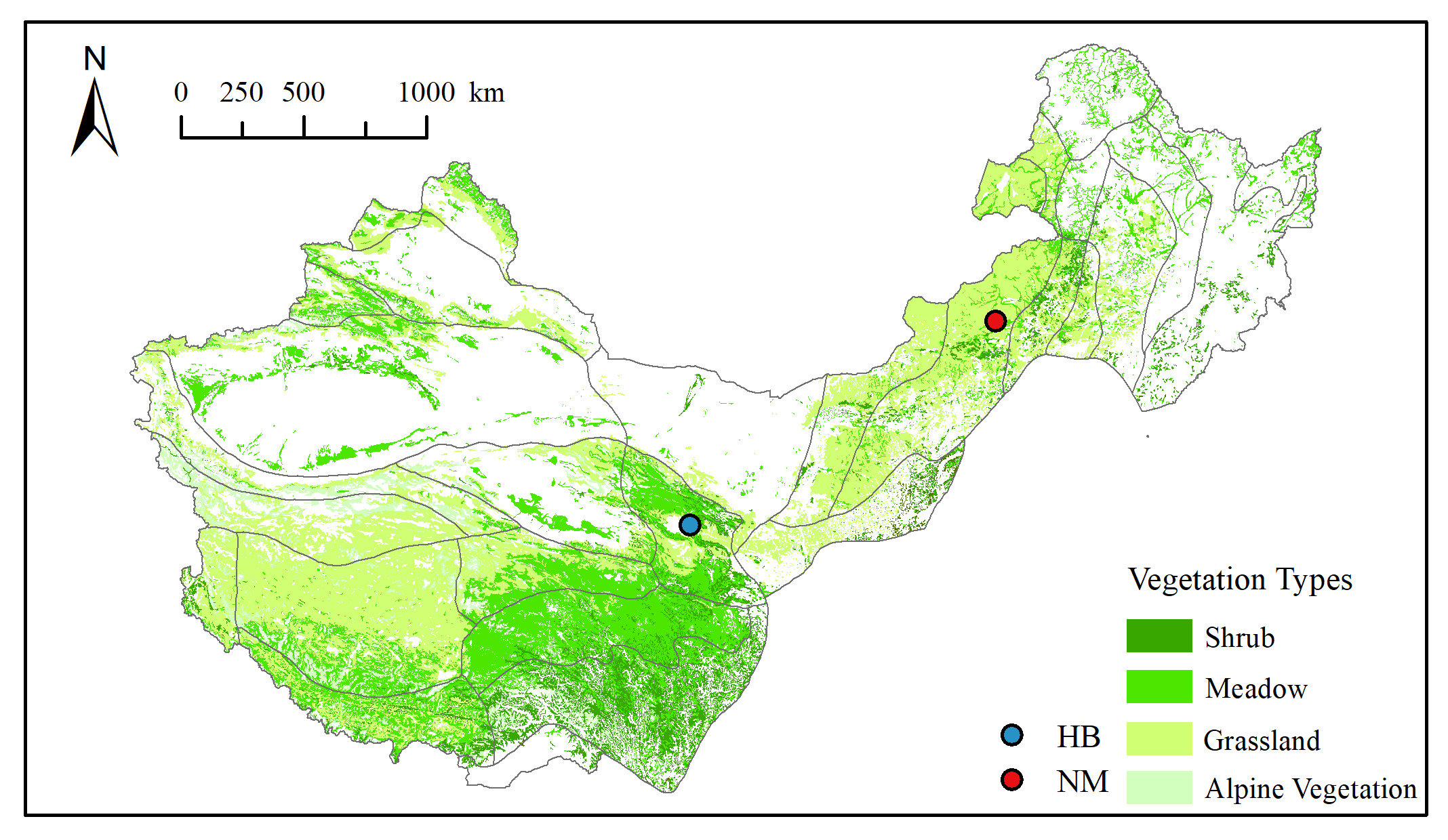
2.1. Site Description

The experimental sites were two typical grassland ecosystems in China: Haibei (HB) and Inner Mongolia (NM), which were near the local grassland ecosystem monitoring stations. The HB Grassland Station is in Xihai county (36°57′N, 100°51′E, elevation 3140 m), Qinghai Autonomous Region (Figure 1). The local area is categorized as plateau monsoon climate with characteristics of strong radiation, low air temperature, and short cool summers. Climatic records from the past five decades show that the average annual air temperature is −0.1 °C, with a coldest monthly mean of −14.1 °C in January and highs of 11.5 °C in July. Average annual precipitation is 391.9 mm, over 80% of which is concentrated between May and September. The dominant species of this alpine meadow grassland are Stipa krylovii, Kobresia humilis, Cleistogenes squarrosa, and Artemisia frigida, and the canopy heights are 20–30 cm. The soil is chestnut soil.
The NM grassland station in Xilinhot, a representative site of the temperate steppe area, is in the Xilin Gol League in the middle of the Inner Mongolia Autonomous Region (43°57′N, 116°07′E, elevation 1003 m) (Figure 1). The climate is semiarid temperate continental climate. The coldest monthly mean of temperature is −18.1 °C in January, and the warmest is 22.5 °C in July. The average annual air temperature is higher than Haibei (2.5 °C), whose ≥0 °C biological accumulated temperature can reach 2350~3400 days per year, but average annual precipitation is lower (273.7 mm). The dominant species of this temperate steppe are Stipa krylovii and Kobresia pygmaea, and the associated species are Leymus chinensis, Cleistogenes squarrosa, Agropyron cristatum, and Artemisia frigida. The soils are sandy loams.

2.2. EC and Meteorological Measurements

EC flux measurements were conducted at the height of 2.0 m in a central fetch of at least 200 m in all directions by open-path EC method [35]. EC flux observations in HB were from 2003 to 2011, and that in NM were from 2004 to 2011, respectively. To avoid potential influences from instrument malfunction, rainfall, dew or cobwebs, human disturbance, and near-static atmospheric conditions, raw measurements were processed and filled according to ChinaFLUX data processing [47,48], which included despiking, coordinate rotation, air density corrections, outlier rejection, and friction velocity threshold (u*) corrections [49]. Based on flux measurements and the exponential relationship between ecosystem respiration (Re) and soil temperature, daytime NEE was partitioned into EC-based GPP as carbon assimilation and Re as carbon emission during daytime (NEE = GPP + Re) [50,51].
Standard meteorological and soil parameters were measured using an array of sensors, including photosynthetically active radiation (PAR), air temperature at the height of 2 m (Ta), precipitation (PPT), air relative humidity (RHa), vapor pressure deficit (VPD), soil temperature at depths of 5 cm (Ts), and soil water content (SWC). All measurements were averaged and recorded in a datalogger once per 30 min. The data were retrieved by a laptop computer every three weeks.

2.3. Phenology Measurements

The phenological monitoring of the dominant vegetation was conducted at the two sites, and the average value of the phenological period (SOS and EOS) of the dominant species in each site was taken as the phenological period of the grassland ecosystem. A 100 m × 100 m vegetation phenological observation field was selected and fenced according to the local grassland types in HB and NM, respectively. The observation field was usually divided into 4 observation areas (50 m × 50 m) as 4 repetitions. Four samples (1 m × 1 m) were randomly selected from each observation area. We selected 10 plants of each dominant species that were growing well and had a complete life history for 3 consecutive years as phenological observation objects. We considered the day of the year (DOY) that over 50% of each species (>5 plants) reached the SOS to the EOS as the phenology periods for the species. The phenological observation was conducted every 2 days for individual plants from SOS to EOS. The phenological observation periods of HB (HB_SOS and HB_EOS) and NM (NM_SOS and NM_EOS) were from 2001 to 2007 and from 2011 to 2017, respectively.

2.4. Remote Data Products

The moderate resolution imaging spectroradiometer (MODIS) Collection 6.0 land products are available from the Land Processes Distributed Active Archive Center (http://daac.ornl.gov/MODIS (accessed on 15 December 2020)). In this study, using two site positions as the center pixel, surface vegetation index products (MOD13Q1), including NDVI and EVI, with a temporal resolution of 16 days and a spatial resolution of 250 m in the last 17 years from January 2001 to December 2017, were extracted. In addition, the surface phenology simulation products (MCD12Q2) from 2001 to 2017 were extracted.

2.5. Phenology Estimation

2.5.1. Threshold Algorithm

In this study, based on the temporal dynamics of NDVI and EVI data in two research sites from 2001 to 2017, we used three methods, including asymmetric Gaussian function (GS), double logistic curve (LG), and Savitzky–Golay (SG) filtering, to fit and reconstruct the smoothing continuous time series of the two stations in TIMESAT software package [52]. According to the smoothed NDVI and EVI time series, the threshold method of TIMESAT software was used to extract the start time (SOS) and end time (EOS) of the growing period in the two stations, respectively. The threshold method is commonly used to simulate vegetation growth and can be expressed as Equation (1):
g ( t ; a 1 , a 2 a 5 ) = exp [ ( t a 1 a 2 ) a 3 ] , t > a 1 g ( t ; a 1 , a 2 a 5 ) = exp [ ( a 1 t a 4 ) a 5 ] , t < a 1
where g(t; a1,a2a5) represents the smoothed NDVI or EVI time series, a1 is the position (day of the year) of the minimum or maximum value of the smoothed temporal NDVI or EVI series, a2 and a3 are the width and flatness of the right half of the series, and a4 and a5 are the width and flatness of the left half of the series. Thus, the phenology estimation of the threshold method can be calculated by the average value of phenology calculated by three filtering method extractions (Figure 2a,c,e,g). The phenological results (SOS and EOS) calculated in HB and NM based on different vegetation indices (NDVI and EVI) are marked as HB_SOS_tn, HB_EOS_tn, HB_SOS_te, HB_EOS_te, and NM_SOS_tn, NM_EOS_tn, NM_SOS_te, NM_EOS_te, respectively (Table 1).

2.5.2. Relative Change Rate Algorithm

In this study, the piecewise logistic function method was used to fit the time series of vegetation indices at two sites [29]. Specifically, the time change of vegetation index in a single growth or senescence cycle can be simulated using Equation (2):
y ( t ) = c 1 + exp ( a + b t ) + d
where y(t) is the NDVI or EVI value at the time of t, a and b are fitting parameters, c + d is the maximum value of NDVI and EVI in the year, and d is the initial value of NDVI and EVI (that is, the minimum value in the year). Among them, the maximum and minimum of the relative change rate of vegetation index are the beginning and ending points of the phenological period (Figure 2b,d,f,h). The phenological results (SOS and EOS) calculated by HB and NM based on different vegetation indices (NDVI and EVI) are marked as HB_SOS_rn, HB_EOS_rn, HB_SOS_re, HB_EOS_re and NM_SOS_rn, NM_EOS_rn, NM_SOS_re, NM_EOS_re, respectively (Table 1).

2.6. Statistical Analysis

The missing values of climate data and vegetation flux observation data were linearly or non-linearly interpolated using their seasonal dynamics. Based on the ground phenological observations in Haibei and Inner Mongolia, the accuracy of remote sensing simulated phenological results, including MODIS product (m), threshold algorithm derived from NDVI and EVI time series (tn and te), and relative change rate algorithm derived from NDVI and EVI time series (rn and re), were investigated by analysis of variance (ANOVA) and multiple comparisons (Tukey’s HSD) (α = 0.05). Linear regression and two statistical parameters, root mean square error (RMSE) and relative prediction error (RPE), were used to quantify the deviation of remote sensing simulation phenology products:
R M S E = i = 1 n ( x i y i ) 2 n
R P E = ( y ¯ x ¯ x ¯ ) × 100 %
where xi is the ground phenological observation, yi is the remote sensing simulated phenological result depending on different methods, and x ¯ and y ¯ are the averages of corresponding data, respectively. The n is the number of samples. Root mean square error (RMSE) is used to measure the bias from the simulated data compared to field measurements. The relative predictive error (RPE) provides the direct effectiveness (underestimation as negative, or overestimation as positive) in predicted values compared to measured values [53]. All statistical and modeling procedures were performed in the R statistical computing package (version 3.5.1).

3. Results

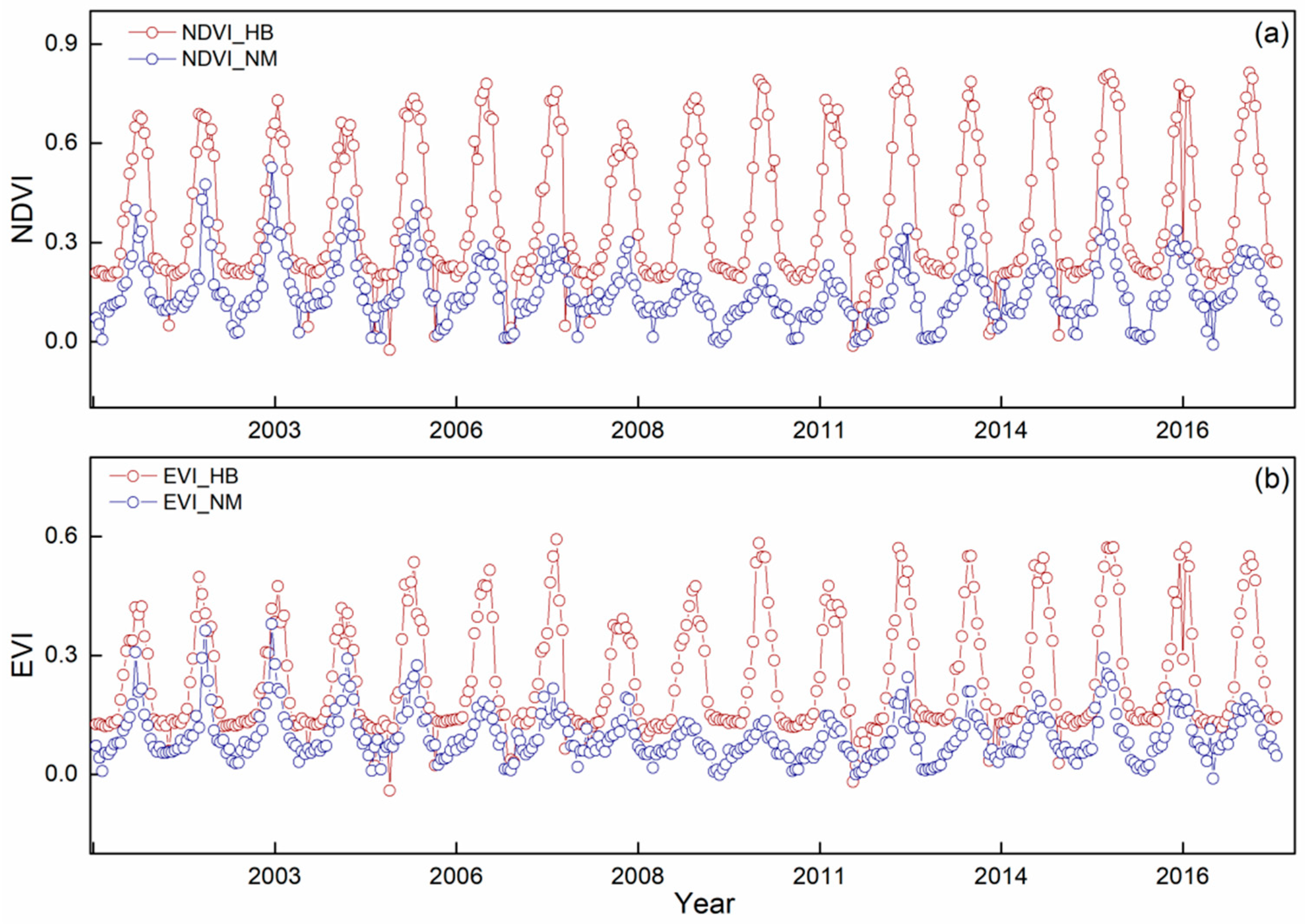
3.1. Vegetation Dynamic

The seasonal variation of GPP and vegetation index (NDVI and EVI) in HB and NM grassland ecosystems showed a single-peak curve change pattern (Figure 3a and Figure 4). The maximum generally appeared at the end of July and early August (DOY200–220), and the productivity and vegetation indexes of HB were significantly higher than those of NM (Figure 3a and Figure 4). The interannual dynamics of productivity in HB and NM both showed a significant upward trend during the study period (HB: R2 = 0.79, NM: R2 = 0.57, p < 0.05) (Figure 3b). In comparison, the annual maximum GPP of HB station appeared in 2010 (1071.99 g C m−2) while the minimum appeared in 2005 and was less than half of 2010 (500.04 g C m−2) (Figure 3b). The maximum value of annual cumulative GPP at the NM station appeared in 2011 (651.77 g C m−2), while the minimum value of approximately half of that in 2011 was in 2009 (325.53 g C m−2) (Figure 3b).
The vegetation productivity in HB improved significantly in the recent 17 years from 2001 to 2017, with a significant increase in annual integrated NDVI and EVI (NDVI: R2 = 0.46, EVI: R2 = 0.68, p < 0.05) (Figure 4). However, the NM station originally showed a significant trend of grassland degradation, and the vegetation growth went through the worst three years from 2009 to 2011, and then it improved again and finally reached close to the initial level in 2001 (Figure 4).
Seasonal variation of vegetation index matched the seasonal dynamics of vegetation (Figure 3a and Figure 4), but the remote sensing estimation of interannual vegetation dynamics was relatively rough (Figure 3b and Figure 4). Specifically, from 2003 to 2011 in HB, the annual integrated vegetation index did not show a significant increase (NDVI: R2 < 0.1, EVI: R2 = 0.16, p > 0.05) despite a significant increase of GPP (Figure 3b). In addition, the divergence in interannual dynamics between vegetation index and GPP was more significant in NM. For example, the vegetation index showed a significant downward trend (NDVI: R2 = 0.9, EVI: R2 = 0.86, p < 0.05) but GPP gradually increased from 2004 to 2011 (Figure 4).

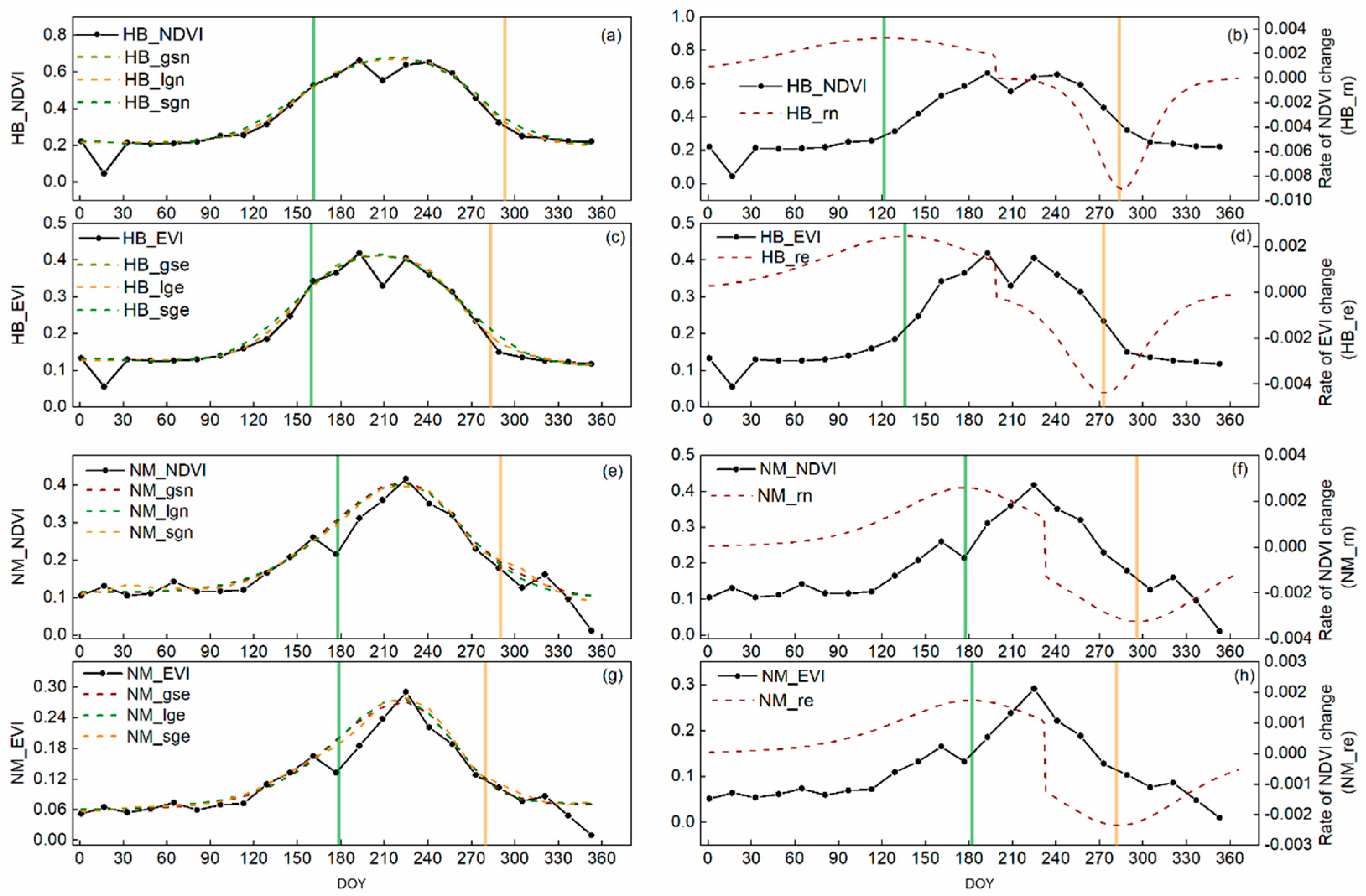
3.2. Vegetation Phenology Dynamic

In this study, a total of six sets of phenological data in HB and NM were obtained using different data and methods (Table 2), which were the phenology measurements on the ground, MODIS products (m), phenological products derived from NDVI and EVI using the threshold method (tn and te) (Figure 2a,c,e,g), and phenological products calculated from NDVI and EVI using the relative rate of change method (rn and re) (Figure 2b,d,f,h, and Table 1).
Different phenological algorithms based on remote sensing indexes significantly overestimated the SOS of HB and NM (p < 0.05) (Table 2), indicating that the phenological simulation based on the remote sensing index of these two sites was not sensitive to SOS. The SOS estimations based on the threshold algorithm had the greatest magnitude of overestimation, especially in HB, where the overestimation reached more than half of the actual value (RPE > 50%, RMSE > 50). Although the phenology estimation calculated from the relative change rate algorithm was relatively improved, there was still a nonnegligible overestimation (RPE < 40%, RMSE < 50). For EOS estimates, the two sites showed different characteristics. For example, the EOS estimations of HB were all overestimated, but the overestimation was obviously smaller than the estimation deviation of SOS (RPE < 10%, RMSE < 20). On the contrary, the EOS simulation based on remote sensing index could provide an unbiased estimate of EOS in NM grassland (p > 0.05, RPE < 5%), especially using the relative change rate algorithm based on EVI data (NM_EOS_re), which could basically accurately estimate the phenological period of NM grassland. (RPE = 0.6%, RMSE = 6.92) (Table 2).
The interannual variation of the actual observed phenological periods (SOS and EOS) in HB and NM could be well simulated by the five different phenological algorithms based on the remote sensing index introduced in this study (b > 0, Figure 4). However, the accuracy of the trend estimation was different. Specifically, in HB grassland, based on NDVI data, the use of threshold and relative rate of change algorithms to simulate the trend of SOS (HB_SOS_tn and HB_SOS_rn) was more accurate (R2 > 0.5, p < 0.05), while other SOS simulation methods were not significant (p > 0.05) (Figure 5a). In contrast, HB_EOS_tn could not effectively assess the interannual variability of EOS in HB grassland (R2 = 0.33, p > 0.1) (Figure 5b). In Inner Mongolia grassland, five different phenological algorithms based on remote sensing index could effectively simulate the interannual variation trend of SOS (R2 > 0.6, p < 0.05) (Figure 5c), but in comparison, only the EOS estimation using the relative change algorithm based on EVI data (NM_EOS_re) could effectively assess the interannual variability of EOS in NM (R2 = 0.7, p = 0.01) (Figure 5d).

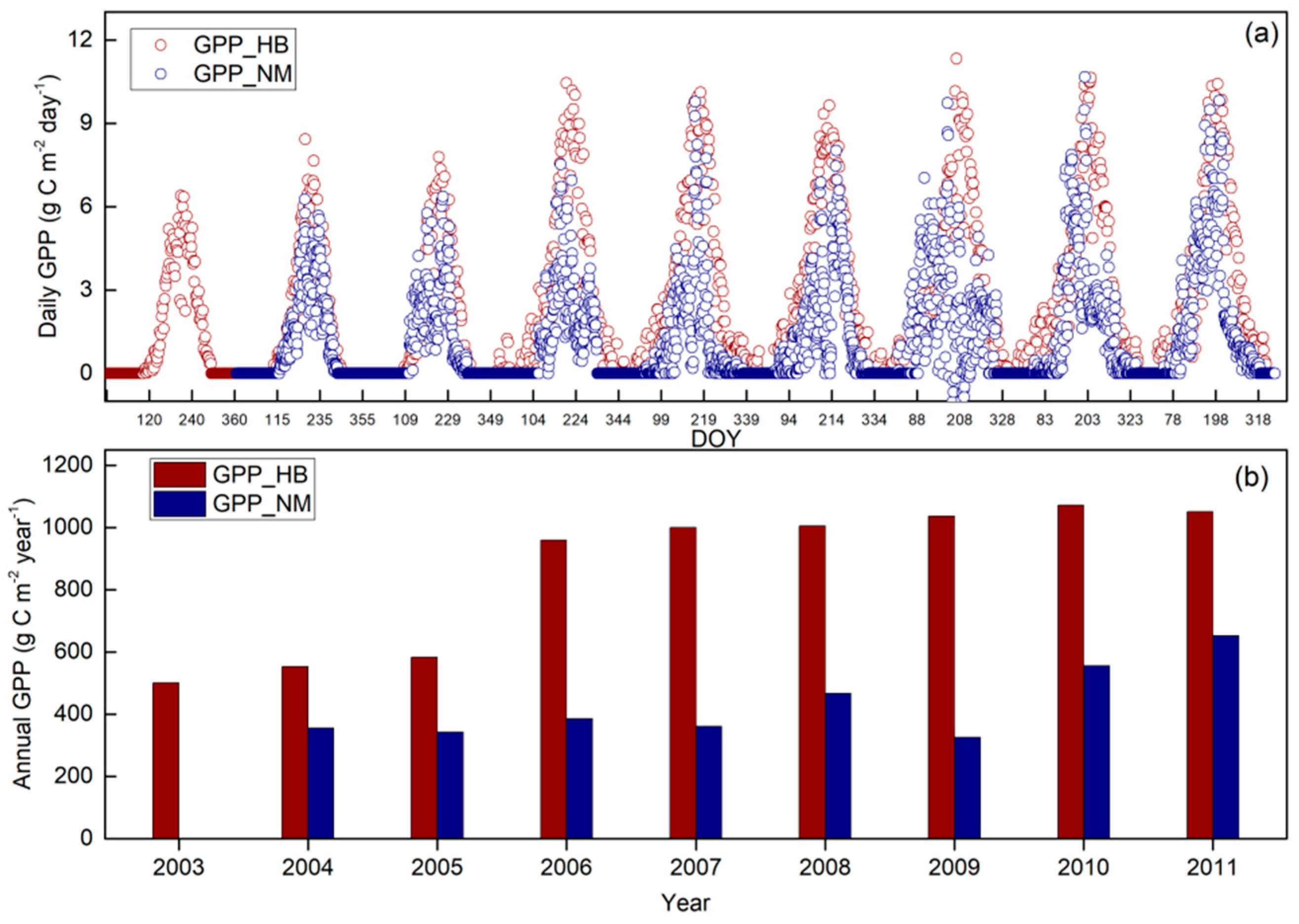
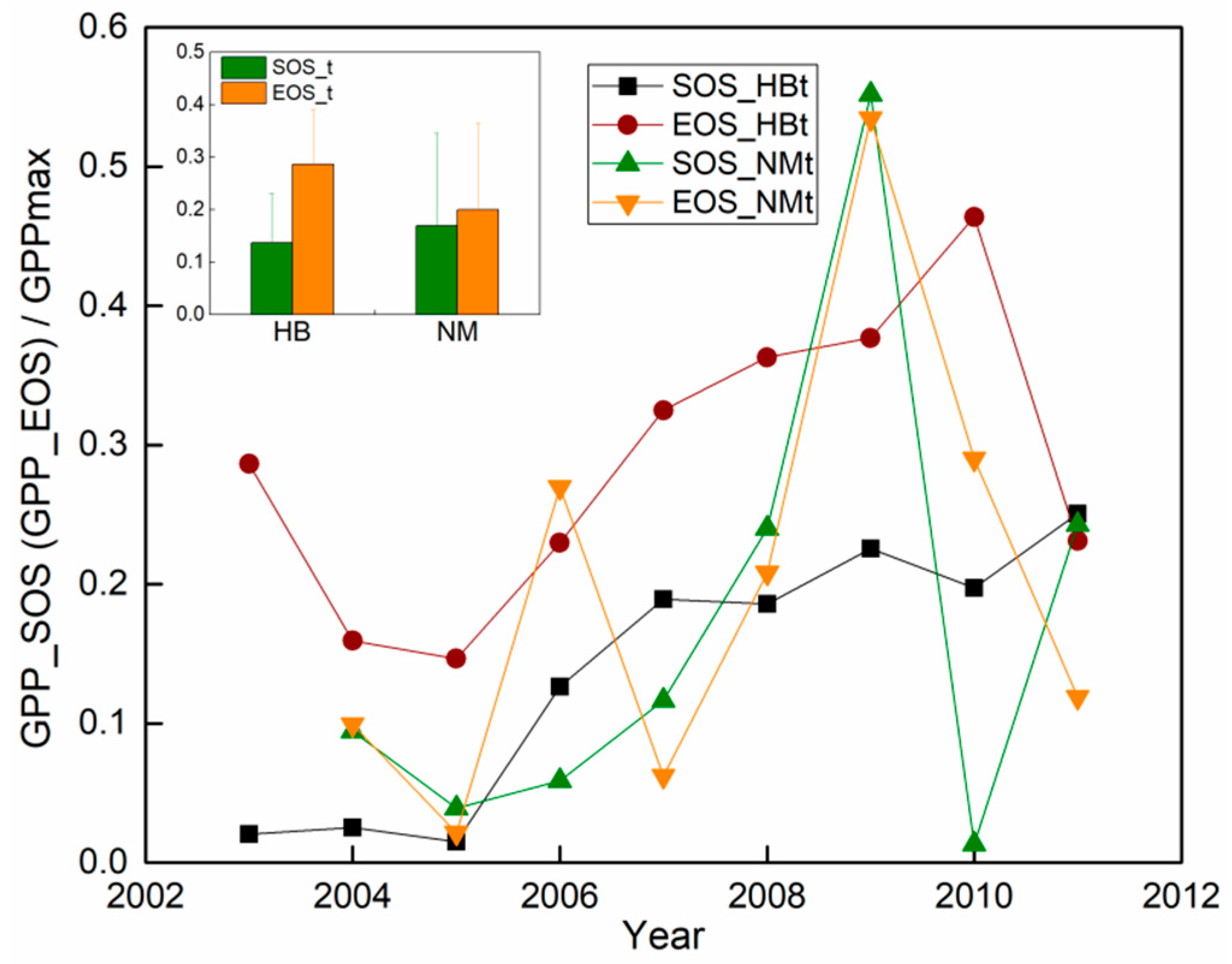
3.3. Carbon Phenology Dynamics

HB_SOS_rn and HB_EOS_rn provided more ideal performance in the estimations of actual phenological values in HB, while NM_SOS_re and NM_EOS_re could more effectively simulate the phenological period of NM (Figure 5a,b). Therefore, we used the actual phenological values in HB and NM to linearly calibrate the value of satellite-based phenology estimations (HB: HB_SOS_rn and HB_EOS_rn (R2 > 0.64, p < 0.05), and NM: NM_SOS_re and NM_EOS_re (R2 = 0.75, p < 0.05), respectively (Figure 6). In addition, the linearly calibrated satellite-based phenology estimations were considered as the correct phenological values in the years when measured phenology values were missing in HB (HB_SOS_c and HB_EOS_c) (Figure 7a) and in NM (NM_SOS_c and NM_EOS_c) (Figure 7b).
As GPP in both two sites in the non-growing season was close to 0, according to the threshold method, the ratio of GPP in the time of SOS (or EOS) and the maximum value of GPP within the year (GPP_max), namely GPP_SOS (or GPP_EOS)/GPP_max, was the threshold of carbon phenology. Therefore, based on similar Savitzky–Golay filtering, daily GPP measurements were smoothed at seasonal scales from 2003 to 2011 in HB (GPP_HBs) and in NM (GPP_NMs) (Figure 7c,d). The maximum value of GPP within the year (GPP_max) was obtained from the smoothed GPP temporal series and combined with the phenological values determined from the actual phenological observations (or the linearly calibrated satellite-based phenology estimations) (Figure 7a,d) to estimate the threshold of carbon phenology in HB and NM, respectively.
The carbon phenology thresholds of grasslands both in HB and NM showed obvious interannual variations (Figure 8). Specifically, during the observation period, the carbon phenology (SOS and EOS) thresholds of HB grassland (HB_SOSt and HB_EOSt) had a significant upward trend, with the multiyear average values being 0.14 and 0.29, respectively. HB_SOSt reached its maximum value in 2010 (0.25). HB_SOSt was relatively smaller in the first three years at the beginning of the observation period, with an average value of 0.02. In contrast, the thresholds of Inner Mongolia grassland (NM_SOSt and NM_EOSt) also had a certain upward trend, but it was not significant (p > 0.05), with the multiyear average values being 0.17 and 0.2, respectively. In addition, the interannual variability of the carbon phenology thresholds in NM was larger than that of HB grassland, with the exception of 2009 when both NM_SOSt and NM_EOSt exceeded 0.5. For the rest of the years, NM_SOSt and NM_EOSt were less than 0.3 (Figure 8).

4. Discussion

4.1. Satellite-Based Vegetation Dynamics

Satellite-based vegetation indexes could match the seasonal dynamics of vegetation growth well, but they were relatively coarse in their estimation of interannual vegetation dynamics (Figure 2 and Figure 3). Most studies also found that satellite-based vegetation indexes and GPP models could capture the intraannual vegetation dynamics well [54,55,56,57,58]. However, assessing interannual vegetation dynamics using satellite-based estimations is full of challenges because of complex interactions between biotic and environmental conditions [56,59,60]. Plant phenology is mainly dependent on intraannual recurring plant growth and reproductive phenomena [61]. Therefore, interannual mismatch between satellite-based vegetation indexes and field observations does not interfere with phenological extraction from satellite-based vegetation dynamics.

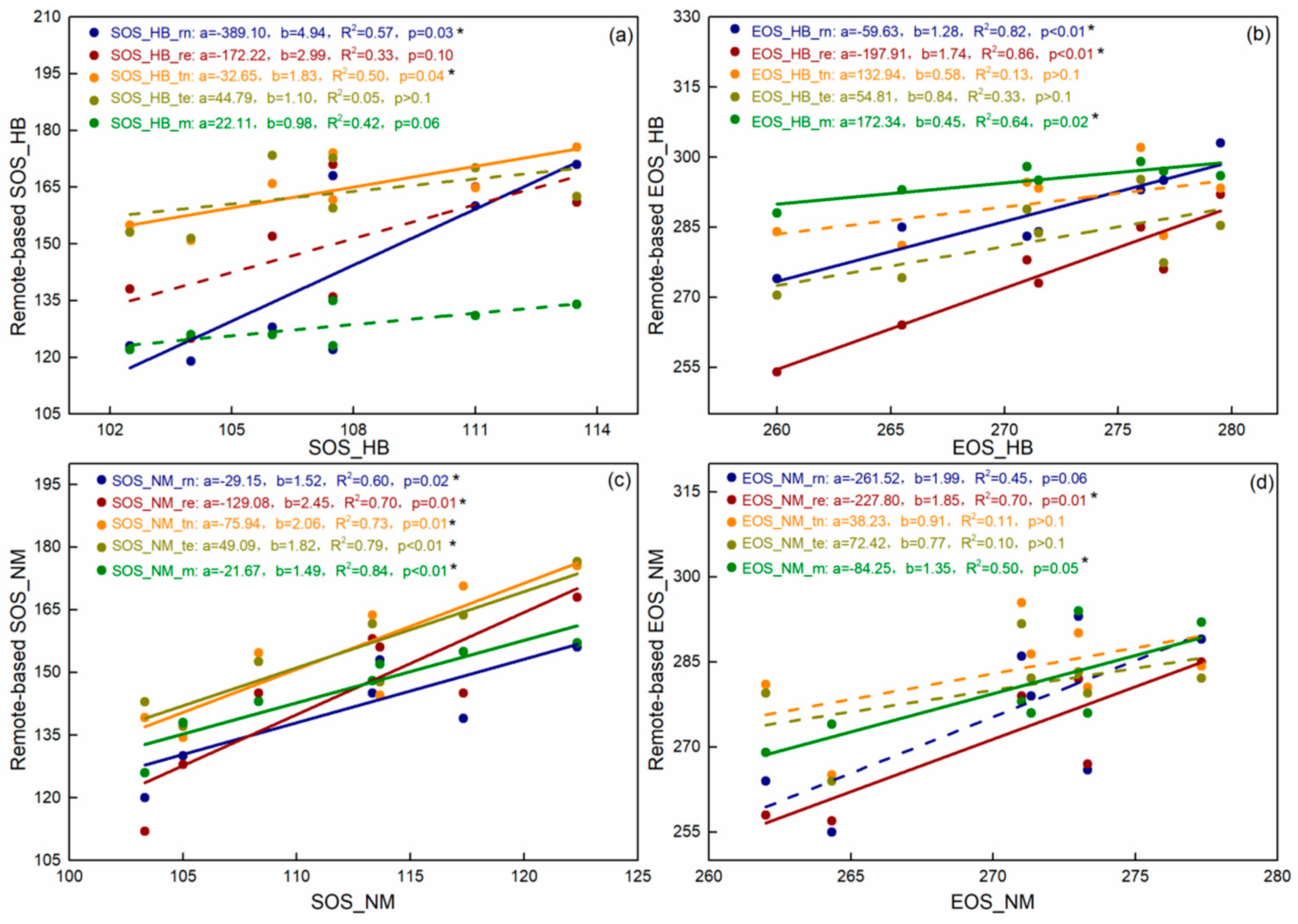
4.2. Satellite-Based Vegetation Phenology Estimations

Satellite-based vegetation phenology estimations (all five of the algorithms in this study) strongly coupled with interannual variations of the actual observed phenological period (Figure 5) but significantly overestimated the SOS in HB and NM (>20% of RPE, Table 2). In other words, the plants had actually entered their growing season, but the satellite-based vegetation phenology estimations did not detect this. Many studies also indicated consistent trends in vegetation phenology between satellite-based phenology estimations and field or near-surface remote observations [22,24,31,32,40,62]. Confounding interferences from the background reflectance of soil, snow, leaf litter, and shadows may lead to these overestimations in satellite-based vegetation phenology [30]. For example, mounds of leaf litter and withered grass in these cold temperate grasslands in the early growing season masked the fact that the plants were turning green [63]. This interference from leaf litter weakened as the vegetation grew taller; thus, satellite-based EOS estimations had a better performance at both sites than SOS estimations (Table 2). Additionally, snow cover and snowmelt remarkably influenced the effect of satellite-based phenology algorithms due to the similar sensitivity of remote-based vegetable indexes to plant greening and snowmelt [19,64,65]. Therefore, field observations and the use of near-surface remote sensing are still necessary to evaluate and refine satellite-based phenology estimates.

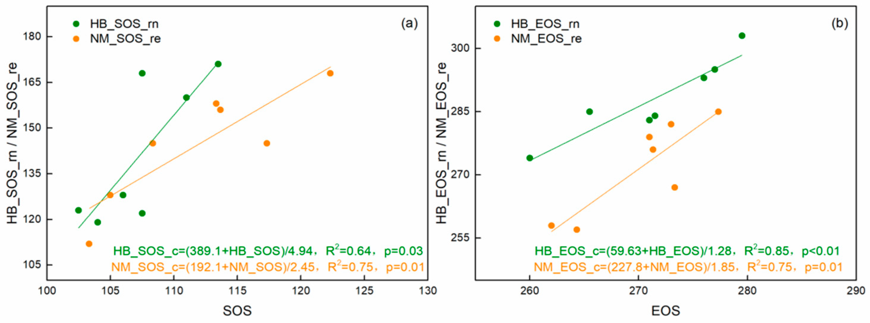
4.3. Vegetation Carbon Phenology and Thresholds

Plant carbon phenology is strongly linked to but not completely equivalent to the natural vegetation phenology period [41,42,43,66,67]. For example, satellite-based SOS estimates from MODIS were highly correlated with the onset of photosynthesis derived from flux measurements despite a later bias for coniferous sites [43]. However, the accuracy in describing annual patterns of flux phenology was generally coarse using satellite-based phenology estimates from different data resources [42]. Thus, most studies found that the trend of vegetation carbon phenology and plant phenology was consistent, but those of absolute dates were not well matched [3,26,42,43]. One reason was due to the uncertainty of satellite-based vegetation phenology estimations and the data quality of EC-based observations [64]. Another possible reason was that the empiric prethreshold settings were not fixed on the space-time scale [68]. Actually, our results showed that there was considerable interannual variation in carbon phenology thresholds in two cold temperate grasslands in China (Figure 8).
Statistically, the EC-based maximum GPP observations (GPPmax) of the year had a significant correlation with the thresholds of carbon phenology periods (SOSt and EOSt) at the HB site (Figure 9a), which provided a simple and valid way to calculate SOSt and EOSt at a specific site and time. Further, the interannual variations of SOSt and EOSt were weakly correlated (Figure 9b), which was largely due to the influence of spring vegetation green-up dates on EOS [1]. The relationship between SOSt and EOSt also implied an alternative way to analyze EOSt variations based on SOSt variations due to a limit of predictive strength in EOS estimation in most phenology studies [1,26,33]. Therefore, this study provided bridges between satellite-based vegetation phenology and EC-based carbon phenology. However, many uncertainties that we did not consider in this study, i.e., agreement of EC-based GPP products with a large footprint and local-scale ground measurements, and the phenology match of specific species and grassland ecosystems across different ecosystems, may have had confounding effects on vegetation carbon phenology and thresholds estimations. Thus, spatial extrapolation to different vegetation types or regions should be based on appropriate validation.

5. Conclusions

This study investigated vegetation phenology in two typical cold temperate grasslands (HB and NM) in China from 2001 to 2017. Compared to ground vegetation phenology observations, we analyzed the performance of MODIS phenology products and two remote sensing-based vegetation phenology algorithms from NDVI and EVI time series. The vegetation phenology estimation from the optimal algorithm was used to calculate the thresholds of carbon phenology periods (SOSt and EOSt) from EC-based GPP observations in each site. Results showed single-peak seasonal variations and significant upward interannual trends of local vegetation growth during the study period in both sites (HB: R2 = 0.79, NM: R2 = 0.57, p < 0.05). Satellite-based phenology estimations (all five algorithms in this study) strongly coupled with temporal variation of the actual observed phenological period but significantly overestimated the SOS, predicting it to be over 21 days later than the field data. The carbon phenology thresholds of HB and NM grasslands showed obvious interannual variations. Specifically, the carbon phenology (SOS and EOS) thresholds of HB grassland (HB_SOSt and HB_EOSt) had a significant upward trend, with the multiyear average values being 0.14 and 0.29, respectively. In contrast, the thresholds of NM grasslands (NM_SOSt and NM_EOSt) also have a certain upward trend but not significant (p > 0.05), with the multiyear average values being 0.17 and 0.2, respectively. Our study suggested the thresholds of carbon phenology periods (SOSt and EOSt) could be simply estimated based on their significant relationship with the EC-based maximum GPP observations (GPPmax) in a specific site and time. However, spatial extrapolation to different vegetation types or regions should be based on appropriate validation.

Author Contributions

L.X. and B.N. conceived and designed the study. B.N., Y.H. and L.X. collected and analyzed the data; X.Z., Y.H., and L.X. contributed observation apparatus; B.N. and L.X. wrote the paper and all other co-authors provided valuable suggestions for the revision. All authors have read and agreed to the published version of the manuscript.

Funding

This work was supported by the National Natural Science Foundation of China (No. 31700421 and No. 41807331), the National Key Research and Development Program (No. 2017YFA0604801), and the West Light Foundation of the Chinese Academy of Sciences (2018).

Conflicts of Interest

The authors declare no conflict of interest.

References

  1. Liu, Q.; Fu, Y.H.; Zhu, Z.; Liu, Y.; Liu, Z.; Huang, M.; Janssens, I.A.; Piao, S. Delayed autumn phenology in the northern hemisphere is related to change in both climate and spring phenology. Glob. Chang. Biol. 2016, 22, 3702–3711. [Google Scholar] [CrossRef]
  2. Churkina, G.; Schimel, D.; Braswell, B.H.; Xiao, X.M. Spatial analysis of growing season length control over net ecosystem exchange. Glob. Chang. Biol. 2005, 11, 1777–1787. [Google Scholar] [CrossRef]
  3. Richardson, A.D.; Andy Black, T.; Ciais, P.; Delbart, N.; Friedl, M.A.; Gobron, N.; Hollinger, D.Y.; Kutsch, W.L.; Longdoz, B.; Luyssaert, S.; et al. Influence of spring and autumn phenological transitions on forest ecosystem productivity. Philos. Trans. R. Soc. B Biol. Sci. 2010, 365, 3227–3246. [Google Scholar] [CrossRef] [Green Version]
  4. Duveneck, M.J.; Thompson, J.R. Climate change imposes phenological trade-offs on forest net primary productivity. J. Geophys. Res. Biogeosci. 2017, 122, 2298–2313. [Google Scholar] [CrossRef]
  5. Piao, S.L.; Friedlingstein, P.; Ciais, P.; Viovy, N.; Demarty, J. Growing season extension and its impact on terrestrial carbon cycle in the northern hemisphere over the past 2 decades. Glob. Biogeochem. Cycles 2007, 21, 1–11. [Google Scholar] [CrossRef]
  6. Cleland, E.E.; Chuine, I.; Menzel, A.; Mooney, H.A.; Schwartz, M.D. Shifting plant phenology in response to global change. Trends Ecol. Evol. 2007, 22, 357–365. [Google Scholar] [CrossRef]
  7. Shen, M.; Piao, S.; Chen, X.; An, S.; Fu, Y.H.; Wang, S.; Cong, N.; Janssens, I.A. Strong impacts of daily minimum temperature on the green-up date and summer greenness of the tibetan plateau. Glob. Chang. Biol. 2016, 22, 3057–3066. [Google Scholar] [CrossRef] [PubMed]
  8. Cong, N.; Shen, M.; Piao, S.; Chen, X.; An, S.; Yang, W.; Fu, Y.H.; Meng, F.; Wang, T. Little change in heat requirement for vegetation green-up on the tibetan plateau over the warming period of 1998–2012. Agric. For. Meteorol. 2017, 232, 650–658. [Google Scholar] [CrossRef]
  9. Prevéy, J.; Vellend, M.; Rüger, N.; Hollister, R.D.; Bjorkman, A.D.; Myers-Smith, I.H.; Elmendorf, S.C.; Clark, K.; Cooper, E.J.; Elberling, B.; et al. Greater temperature sensitivity of plant phenology at colder sites: Implications for convergence across northern latitudes. Glob. Chang. Biol. 2017, 23, 2660–2671. [Google Scholar] [CrossRef] [PubMed] [Green Version]
  10. Zhang, Q.; Kong, D.; Shi, P.; Singh, V.P.; Sun, P. Vegetation phenology on the qinghai-tibetan plateau and its response to climate change (1982–2013). Agric. For. Meteorol. 2018, 248, 408–417. [Google Scholar] [CrossRef]
  11. Schwartz, M.D.; Ahas, R.; Aasa, A. Onset of spring starting earlier across the northern hemisphere. Glob. Chang. Biol. 2006, 12, 343–351. [Google Scholar] [CrossRef]
  12. Shen, M.; Zhang, G.; Cong, N.; Wang, S.; Kong, W.; Piao, S. Increasing altitudinal gradient of spring vegetation phenology during the last decade on the qinghai–tibetan plateau. Agric. For. Meteorol. 2014, 189–190, 71–80. [Google Scholar] [CrossRef]
  13. Garonna, I.; de Jong, R.; Schaepman, M.E. Variability and evolution of global land surface phenology over the past three decades (1982–2012). Glob. Chang. Biol. 2016, 22, 1456–1468. [Google Scholar] [CrossRef]
  14. Piao, S.; Liu, Q.; Chen, A.; Janssens, I.A.; Fu, Y.; Dai, J.; Liu, L.; Lian, X.; Shen, M.; Zhu, X. Plant phenology and global climate change: Current progresses and challenges. Glob. Chang. Biol. 2019, 25, 1922–1940. [Google Scholar] [CrossRef]
  15. Piao, S.L.; Cui, M.D.; Chen, A.P.; Wang, X.H.; Ciais, P.; Liu, J.; Tang, Y.H. Altitude and temperature dependence of change in the spring vegetation green-up date from 1982 to 2006 in the qinghai-xizang plateau. Agric. For. Meteorol. 2011, 151, 1599–1608. [Google Scholar] [CrossRef]
  16. Shen, M.; Piao, S.; Dorji, T.; Liu, Q.; Cong, N.; Chen, X.; An, S.; Wang, S.; Wang, T.; Zhang, G. Plant phenological responses to climate change on the tibetan plateau: Research status and challenges. Natl. Sci. Rev. 2015, 2, 454–467. [Google Scholar] [CrossRef] [Green Version]
  17. Luo, Y.; El-Madany, T.; Ma, X.; Nair, R.; Jung, M.; Weber, U.; Filippa, G.; Bucher, S.F.; Moreno, G.; Cremonese, E.; et al. Nutrients and water availability constrain the seasonality of vegetation activity in a mediterranean ecosystem. Glob. Chang. Biol. 2020, 26, 4379–4400. [Google Scholar] [CrossRef] [PubMed]
  18. Wang, H.; Liu, D.; Lin, H.; Montenegro, A.; Zhu, X. Ndvi and vegetation phenology dynamics under the influence of sunshine duration on the tibetan plateau. Int. J. Climatol. 2015, 35, 687–698. [Google Scholar] [CrossRef]
  19. Wang, S.; Wang, X.; Chen, G.; Yang, Q.; Wang, B.; Ma, Y.; Shen, M. Complex responses of spring alpine vegetation phenology to snow cover dynamics over the tibetan plateau, china. Sci. Total Environ. 2017, 593–594, 449–461. [Google Scholar] [CrossRef] [PubMed]
  20. Ganjurjav, H.; Gornish, E.S.; Hu, G.; Schwartz, M.W.; Wan, Y.; Li, Y.; Gao, Q. Warming and precipitation addition interact to affect plant spring phenology in alpine meadows on the central qinghai-tibetan plateau. Agric. For. Meteorol. 2020, 287, 107943. [Google Scholar] [CrossRef]
  21. Ding, C.; Liu, X.; Huang, F.; Li, Y.; Zou, X. Onset of drying and dormancy in relation to water dynamics of semi-arid grasslands from modis ndwi. Agric. For. Meteorol. 2017, 234–235, 22–30. [Google Scholar] [CrossRef]
  22. Liu, Y.; Hill, M.J.; Zhang, X.; Wang, Z.; Richardson, A.D.; Hufkens, K.; Filippa, G.; Baldocchi, D.D.; Ma, S.; Verfaillie, J.; et al. Using data from landsat, modis, viirs and phenocams to monitor the phenology of california oak/grass savanna and open grassland across spatial scales. Agric. For. Meteorol. 2017, 237–238, 311–325. [Google Scholar] [CrossRef]
  23. Shang, R.; Liu, R.; Xu, M.; Liu, Y.; Zuo, L.; Ge, Q. The relationship between threshold-based and inflexion-based approaches for extraction of land surface phenology. Remote Sens. Environ. 2017, 199, 167–170. [Google Scholar] [CrossRef]
  24. Jenkins, J.P.; Braswell, B.H.; Frolking, S.E.; Aber, J.D. Detecting and predicting spatial and interannual patterns of temperate forest springtime phenology in the eastern U.S. Geophys. Res. Lett. 2002, 29, 54-1–54-4. [Google Scholar] [CrossRef] [Green Version]
  25. Piao, S.; Fang, J.; Zhou, L.; Ciais, P.; Zhu, B. Variations in satellite-derived phenology in China’s temperate vegetation. Glob. Chang. Biol. 2006, 12, 672–685. [Google Scholar] [CrossRef]
  26. Wu, C.; Peng, D.; Soudani, K.; Siebicke, L.; Gough, C.M.; Arain, M.A.; Bohrer, G.; Lafleur, P.M.; Peichl, M.; Gonsamo, A.; et al. Land surface phenology derived from normalized difference vegetation index (ndvi) at global fluxnet sites. Agric. For. Meteorol. 2017, 233, 171–182. [Google Scholar] [CrossRef]
  27. White, M.A.; Nemani, R.R. Real-time monitoring and short-term forecasting of land surface phenology. Remote Sens. Environ. 2006, 104, 43–49. [Google Scholar] [CrossRef]
  28. Wang, S.; Zhang, B.; Yang, Q.; Chen, G.; Yang, B.; Lu, L.; Shen, M.; Peng, Y. Responses of net primary productivity to phenological dynamics in the tibetan plateau, china. Agric. For. Meteorol. 2017, 232, 235–246. [Google Scholar] [CrossRef]
  29. Zhang, X.; Friedl, M.A.; Schaaf, C.B.; Strahler, A.H.; Hodges, J.C.F.; Gao, F.; Reed, B.C.; Huete, A. Monitoring vegetation phenology using modis. Remote Sens. Environ. 2003, 84, 471–475. [Google Scholar] [CrossRef]
  30. Yang, W.; Kobayashi, H.; Wang, C.; Shen, M.; Chen, J.; Matsushita, B.; Tang, Y.; Kim, Y.; Bret-Harte, M.S.; Zona, D.; et al. A semi-analytical snow-free vegetation index for improving estimation of plant phenology in tundra and grassland ecosystems. Remote Sens. Environ. 2019, 228, 31–44. [Google Scholar] [CrossRef]
  31. Klosterman, S.T.; Hufkens, K.; Gray, J.M.; Melaas, E.; Sonnentag, O.; Lavine, I.; Mitchell, L.; Norman, R.; Friedl, M.A.; Richardson, A.D. Evaluating remote sensing of deciduous forest phenology at multiple spatial scales using phenocam imagery. Biogeosciences 2014, 11, 4305–4320. [Google Scholar] [CrossRef] [Green Version]
  32. Liu, Z.; Wu, C.; Liu, Y.; Wang, X.; Fang, B.; Yuan, W.; Ge, Q. Spring green-up date derived from gimms3g and spot-vgt ndvi of winter wheat cropland in the north china plain. ISPRS J. Photogramm. Remote Sens. 2017, 130, 81–91. [Google Scholar] [CrossRef]
  33. Wu, C.; Wang, X.; Wang, H.; Ciais, P.; Peñuelas, J.; Myneni, R.B.; Desai, A.R.; Gough, C.M.; Gonsamo, A.; Black, A.T.; et al. Contrasting responses of autumn-leaf senescence to daytime and night-time warming. Nat. Clim. Chang. 2018, 8, 1092–1096. [Google Scholar] [CrossRef] [Green Version]
  34. White, K.; Pontius, J.; Schaberg, P. Remote sensing of spring phenology in northeastern forests: A comparison of methods, field metrics and sources of uncertainty. Remote Sens. Environ. 2014, 148, 97–107. [Google Scholar] [CrossRef]
  35. Baldocchi, D. Measuring biosphere-atmosphere exchange of biologically ralated gases with micrometeorological methods. Ecology 1988, 65, 1331–1340. [Google Scholar] [CrossRef]
  36. Reichstein, M.; Falge, E.; Baldocchi, D.; Papale, D.; Aubinet, M.; Berbigier, P.; Bernhofer, C.; Buchmann, N.; Gilmanov, T.; Granier, A.; et al. On the separation of net ecosystem exchange into assimilation and ecosystem respiration: Review and improved algorithm. Glob. Chang. Biol. 2005, 11, 1424–1439. [Google Scholar] [CrossRef]
  37. Hanan, N.P.; Burba, G.; Verma, S.B.; Berry, J.A.; Suyker, A.; Walter-Shea, E.A. Inversion of net ecosystem CO2 flux measurements for estimation of canopy par absorption. Glob. Chang. Biol. 2002, 8, 563–574. [Google Scholar] [CrossRef]
  38. Reichstein, M.; Ciais, P.; Papale, D.; Valentini, R.; Running, S.; Viovy, N.; Cramer, W.; Granier, A.; OgÉE, J.; Allard, V.; et al. Reduction of ecosystem productivity and respiration during the european summer 2003 climate anomaly: A joint flux tower, remote sensing and modelling analysis. Glob. Chang. Biol. 2007, 13, 634–651. [Google Scholar] [CrossRef]
  39. Friend, A.D.; Arneth, A.; Kiang, N.Y.; Lomas, M.; OgÉE, J.; RÖDenbeck, C.; Running, S.W.; Santaren, J.-D.; Sitch, S.; Viovy, N.; et al. Fluxnet and modelling the global carbon cycle. Glob. Chang. Biol. 2007, 13, 610–633. [Google Scholar] [CrossRef]
  40. Peng, D.; Zhang, X.; Wu, C.; Huang, W.; Gonsamo, A.; Huete, A.R.; Didan, K.; Tan, B.; Liu, X.; Zhang, B. Intercomparison and evaluation of spring phenology products using national phenology network and ameriflux observations in the contiguous united states. Agric. For. Meteorol. 2017, 242, 33–46. [Google Scholar] [CrossRef] [Green Version]
  41. Baldocchi, D.D.; Black, T.A.; Curtis, P.S.; Falge, E.; Fuentes, J.D.; Granier, A.; Gu, L.; Knohl, A.; Pilegaard, K.; Schmid, H.P.; et al. Predicting the onset of net carbon uptake by deciduous forests with soil temperature and climate data: A synthesis of fluxnet data. Int. J. Biometeorol. 2005, 49, 377–387. [Google Scholar] [CrossRef]
  42. Garrity, S.R.; Bohrer, G.; Maurer, K.D.; Mueller, K.L.; Vogel, C.S.; Curtis, P.S. A comparison of multiple phenology data sources for estimating seasonal transitions in deciduous forest carbon exchange. Agric. For. Meteorol. 2011, 151, 1741–1752. [Google Scholar] [CrossRef]
  43. Melaas, E.K.; Richardson, A.D.; Friedl, M.A.; Dragoni, D.; Gough, C.M.; Herbst, M.; Montagnani, L.; Moors, E. Using fluxnet data to improve models of springtime vegetation activity onset in forest ecosystems. Agric. For. Meteorol. 2013, 171–172, 46–56. [Google Scholar] [CrossRef]
  44. Fan, J.; Zhong, H.; Harris, W.; Yu, G.; Wang, S.; Hu, Z.; Yue, Y. Carbon storage in the grasslands of china based on field measurements of above- and below-ground biomass. Clim. Chang. 2008, 86, 375–396. [Google Scholar] [CrossRef]
  45. Scurlock, J.M.O.; Hall, D.O. The global carbon sink: A grassland perspective. Glob. Chang. Biol. 1998, 4, 229–233. [Google Scholar] [CrossRef] [Green Version]
  46. Ni, J. Carbon storage in grasslands of china. J. Arid Environ. 2002, 50, 205–218. [Google Scholar] [CrossRef]
  47. Li, C.; He, H.L.; Liu, M.; Su, W.; Fu, Y.L.; Zhang, L.M.; Wen, X.F.; Yu, G.R. The design and application of CO2 flux data processing system at chinaflux. Geo-Inf. Sci. 2008, 10, 557–565. [Google Scholar]
  48. Yu, G.R.; Wen, X.F.; Sun, X.M.; Tanner, B.D.; Lee, X.H.; Chen, J.Y. Overview of chinaflux and evaluation of its eddy covariance measurement. Agric. For. Meteorol. 2006, 137, 125–137. [Google Scholar] [CrossRef]
  49. Niu, B.; He, Y.; Zhang, X.; Du, M.; Shi, P.; Sun, W.; Zhang, L. CO2 exchange in an alpine swamp meadow on the central tibetan plateau. Wetlands 2017, 37, 525–543. [Google Scholar] [CrossRef]
  50. Lasslop, G.; Reichstein, M.; Papale, D.; Richardson, A.D.; Arneth, A.; Barr, A.; Stoy, P.; Wohlfahrt, G. Separation of net ecosystem exchange into assimilation and respiration using a light response curve approach: Critical issues and global evaluation. Glob. Chang. Biol. 2010, 16, 187–208. [Google Scholar] [CrossRef] [Green Version]
  51. Niu, B.; He, Y.; Zhang, X.; Zong, N.; Fu, G.; Shi, P.; Zhang, Y.; Du, M.; Zhang, J. Satellite-based inversion and field validation of autotrophic and heterotrophic respiration in an alpine meadow on the tibetan plateau. Remote Sens. 2017, 9, 615. [Google Scholar] [CrossRef] [Green Version]
  52. Jönsson, P.; Eklundh, L. Timesat—a program for analyzing time-series of satellite sensor data. Comput. Geosci. 2004, 30, 833–845. [Google Scholar] [CrossRef] [Green Version]
  53. Kanniah, K.D.; Beringer, J.; Hutley, L.B.; Tapper, N.J.; Zhu, X. Evaluation of collections 4 and 5 of the modis gross primary productivity product and algorithm improvement at a tropical savanna site in northern australia. Remote Sens. Environ. 2009, 113, 1808–1822. [Google Scholar] [CrossRef]
  54. Dong, J.; Xiao, X.; Wagle, P.; Zhang, G.; Zhou, Y.; Jin, C.; Torn, M.S.; Meyers, T.P.; Suyker, A.E.; Wang, J.; et al. Comparison of four evi-based models for estimating gross primary production of maize and soybean croplands and tallgrass prairie under severe drought. Remote Sens. Environ. 2015, 162, 154–168. [Google Scholar] [CrossRef] [Green Version]
  55. Niu, B.; He, Y.; Zhang, X.; Fu, G.; Shi, P.; Du, M.; Zhang, Y.; Zong, N. Tower-based validation and improvement of modis gross primary production in an alpine swamp meadow on the tibetan plateau. Remote Sens. 2016, 8, 592. [Google Scholar] [CrossRef] [Green Version]
  56. Verma, M.; Friedl, M.A.; Law, B.E.; Bonal, D.; Kiely, G.; Black, T.A.; Wohlfahrt, G.; Moors, E.J.; Montagnani, L.; Marcolla, B.; et al. Improving the performance of remote sensing models for capturing intra- and inter-annual variations in daily gpp: An analysis using global fluxnet tower data. Agric. For. Meteorol. 2015, 214–215, 416–429. [Google Scholar] [CrossRef] [Green Version]
  57. Wu, C.; Chen, J.M.; Desai, A.R.; Hollinger, D.Y.; Arain, M.A.; Margolis, H.A.; Gough, C.M.; Staebler, R.M. Remote sensing of canopy light use efficiency in temperate and boreal forests of north america using modis imagery. Remote Sens. Environ. 2012, 118, 60–72. [Google Scholar] [CrossRef]
  58. Niu, B.; Zhang, X.; He, Y.; Shi, P.; Fu, G.; Du, M.; Zhang, Y.; Zong, N.; Zhang, J.; Wu, J. Satellite-based estimation of gross primary production in an alpine swamp meadow on the tibetan plateau: A multi-model comparison. J. Resour. Ecol. 2017, 8, 57–66. [Google Scholar]
  59. Wohlfahrt, G.; Anderson-Dunn, M.; Bahn, M.; Balzarolo, M.; Berninger, F.; Campbell, C.; Carrara, A.; Cescatti, A.; Christensen, T.; Dore, S.; et al. Biotic, abiotic, and management controls on the net ecosystem CO2 exchange of european mountain grassland ecosystems. Ecosystems 2008, 11, 1338–1351. [Google Scholar] [CrossRef]
  60. Kato, T.; Tang, Y.; Gu, S.; Hirota, M.; Du, M.; Li, Y.; Zhao, X. Temperature and biomass influences on interannual changes in CO2 exchange in an alpine meadow on the qinghai-tibetan plateau. Glob. Chang. Biol. 2006, 12, 1285–1298. [Google Scholar] [CrossRef]
  61. Forrest, J.; Miller-Rushing, A.J. Toward a synthetic understanding of the role of phenology in ecology and evolution. Philos. Trans. R. Soc. Lond. Ser. B Biol. Sci. 2010, 365, 3101–3112. [Google Scholar] [CrossRef] [PubMed] [Green Version]
  62. Hufkens, K.; Friedl, M.; Sonnentag, O.; Braswell, B.H.; Milliman, T.; Richardson, A.D. Linking near-surface and satellite remote sensing measurements of deciduous broadleaf forest phenology. Remote Sens. Environ. 2012, 117, 307–321. [Google Scholar] [CrossRef]
  63. Li, G.; Jiang, C.; Cheng, T.; Bai, J. Grazing alters the phenology of alpine steppe by changing the surface physical environment on the northeast qinghai-tibet plateau, china. J. Environ. Manag. 2019, 248, 109257. [Google Scholar] [CrossRef]
  64. Gonsamo, A.; Chen, J.M.; Price, D.T.; Kurz, W.A.; Wu, C. Land surface phenology from optical satellite measurement and CO2 eddy covariance technique. J. Geophys. Res. Biogeosci. 2012, 117, 1–18. [Google Scholar] [CrossRef]
  65. Huang, K.; Zhang, Y.; Tagesson, T.; Brandt, M.; Wang, L.; Chen, N.; Zu, J.; Jin, H.; Cai, Z.; Tong, X.; et al. The confounding effect of snow cover on assessing spring phenology from space: A new look at trends on the tibetan plateau. Sci. Total Environ. 2021, 756, 144011. [Google Scholar] [CrossRef]
  66. Wohlfahrt, G.; Cremonese, E.; Hammerle, A.; Hörtnagl, L.; Galvagno, M.; Gianelle, D.; Marcolla, B.; di Cella, U.M. Trade-offs between global warming and day length on the start of the carbon uptake period in seasonally cold ecosystems. Geophys. Res. Lett. 2013, 40, 6136–6142. [Google Scholar] [CrossRef]
  67. Lang, W.; Chen, X.; Qian, S.; Liu, G.; Piao, S. A new process-based model for predicting autumn phenology: How is leaf senescence controlled by photoperiod and temperature coupling? Agric. For. Meteorol. 2019, 268, 124–135. [Google Scholar] [CrossRef]
  68. Meng, F.; Zhou, Y.; Wang, S.; Duan, J.; Zhang, Z.; Niu, H.; Jiang, L.; Cui, S.; Li, X.E.; Luo, C.; et al. Temperature sensitivity thresholds to warming and cooling in phenophases of alpine plants. Clim. Chang. 2016, 139, 579–590. [Google Scholar] [CrossRef]
Figure 1. The geographical locations and vegetation types of the two sites, Haibei (HB) and Inner Mongolia (NM), in this study.
Remotesensing 13 00574 g001
Figure 2. Examples of different methods for calculating vegetation phenology in Haibei (HB) and Inner Mongolia (NM) grassland stations (2004). The phenological period of vegetation in HB (ad) and NM (eh) are estimated by threshold method (left column) and relative change rate method (right column). For the threshold method, three filters, including asymmetric Gaussian function (GS), double logistic curve (LG), and Savitzky–Golay (SG) filtering, are used to fit and reconstruct the smoothing continuous time series of normalized difference vegetation index (NDVI) and enhanced vegetation index (EVI). The green and yellow lines represent the start time (SOS) and end time (EOS) of the growing period for the year, respectively.
Remotesensing 13 00574 g002
Figure 3. Seasonal (a) and interannual dynamics (b) of EC-based gross primary productivity (GPP) in Haibei (HB) and Inner Mongolia (NM) grassland stations from 2003 to 2011.
Remotesensing 13 00574 g003
Figure 4. Seasonal (a) and interannual dynamics (b) of MODIS vegetation index (NDVI and EVI) in Haibei (HB) and Inner Mongolia (NM) grassland stations from 2001 to 2017.
Remotesensing 13 00574 g004
Figure 5. Verification of the accuracy of five different methods for calculating vegetation phenological period in Haibei (HB) and Inner Mongolia (NM) grasslands based on field phenology observations. b values in (ad) are the linear slope between field phenology observations and satellite-based phenology estimations, respectively. All solid lines are significant trends (p < 0.01) and the dash lines are nonsignificant trends (p > 0.05). Colors in (ad) are one-to-one corresponding with five satellite-based phenology estimations (Table 2).
Remotesensing 13 00574 g005
Figure 6. The linearly calibrated satellite-based phenology estimations from the actual phenological observations in HB and NM. (a,b) are the day of the start and end of growing season (SOS and EOS) calibration, respectively.
Remotesensing 13 00574 g006
Figure 7. Interannual variability of the vegetation phenology periods (a,b), and an example on the determination of the threshold of carbon phenology periods in HB and NM (c,d) (2004). Solid points and lines represent field actual phenological values, and the dashed points and lines are the calibrated satellite-based phenology estimations in HB (a) and NM (b) based on field actual phenological observations. The green and yellow lines represent the SOS and EOS of the year in HB (c) and in NM (d) grasslands, respectively.
Remotesensing 13 00574 g007
Figure 8. Interannual dynamics of vegetation carbon phenological period thresholds (%) in HB and NM grasslands from 2003 to 2011. The inset chart shows the mean values of annual vegetation carbon phenological period thresholds in HB and NM, and the green and yellow bars represent the SOS and EOS of the year in HB and in NM grasslands, respectively.
Remotesensing 13 00574 g008
Figure 9. The determination of the thresholds of carbon phenology periods from EC-based maximum GPP observations (GPPmax) in HB (a) and the relationship between two thresholds of carbon phenology periods (SOSt and EOSt) in HB and NM sites (b). The solid line represents a significant regression relationship (p < 0.05).
Remotesensing 13 00574 g009
Table 1. Acronyms and their descriptions in this study.
AcronymsDescriptions
HB and NMTwo cold temperate grassland sites in Haibei and Inner Mongolia.
NDVI and EVITwo surface vegetation index products from MOD13Q1.
SOS and EOSThe timing of the start and the end of the vegetation growing season.
tn and teThreshold based phenology estimation derived from NDVI and EVI.
rn and reRelative change rate based phenology derived from NDVI and EVI.
mThe surface phenology simulation products (MCD12Q2).
RMSE and RPERoot mean square error and relative prediction error.
SOS_c and EOS_cCalibrated satellite SOS and EOS based on the actual phenological observations.
SOSt and EOStThe vegetation carbon phenological period thresholds (%) of SOS and EOS.
Table 2. Comparison of the estimation of interannual mean of the vegetation phenology period with different methods.
SiteMethod *Mean (1 Standard Deviation) **RMSERPE (%) ***
SOSEOSSOSEOSSOSEOS
HBField108 (4)a272 (7)a0000
m129 (6)b296 (4)c20.9823.97−19.3−8.7
tn164 (10)d291 (8)c56.8819.86−52.6−6.9
te164 (9)d283 (9)ac56.3212.28−51.9− 3.9
rn142 (23)bc289 (10)bc39.1117.08−31.8−6.1
re150 (17)cd275 (13)ab44.466.84−39.4−1.1
NMField110 (6)a271 (6)a0000
m137 (13)b288 (11)a34.0011.19−30.1−3.5
tn159 (14)b287 (9)a43.8515.04−38.2−4.8
te159 (12)b281 (9)a43.3112.05−38.1−3.6
rn141 (18)b282 (13)a29.9011.74−25.8−2.1
re147 (17)b273 (11)a35.026.92−29.1−0.6
* Field, m, tn, te, rn, and re represent phenology measurements on the ground, MODIS phenology product (m), phenological products derived from NDVI and EVI using the threshold method (tn and te), and the relative rate of change method (rn and re), respectively. ** Different letters in the same column indicate significant differences in phenological estimation by different methods (p < 0.05) in HB and NM, respectively. *** The negative value of RPE means that the remote sensing phenological estimation method overestimates the measured values.
Publisher’s Note: MDPI stays neutral with regard to jurisdictional claims in published maps and institutional affiliations.

