1. Introduction
Cloud radars are a helpful tool for studying differences in the structure of convective storms with or without the occurrence of lightning. The differences in the structure of convective storms obtained in the measured radar data provide information, which helps to understand the processes taking place in clouds. One of the key processes occurring in thunderclouds is the process of electrification, which precedes lightning discharges. Although cloud radars cannot explicitly measure the origin and the evolution of electrification of clouds, they can describe it indirectly; using derived or directly measured radar data. It is important that the cloud radars are polarimetric to be used in the research of cloud electrification.
Cloud radars are not the only or the most important source of data on cloud electrification and related lightning discharges. Useful data are also obtained from laboratory experiments [
1,
2] and measurement campaigns performed in the field through areas in thunderclouds (e.g., balloon experiments, devices on board aircrafts) [
3,
4,
5,
6,
7]. Further, data on lightning discharges are available as ground observations or from satellites [
8,
9,
10,
11,
12,
13].
A few papers has been published that used cloud radars for the investigation of cloud electrification. These were mainly focused on the alignment of cloud particles in intensified electrostatic field [
14,
15,
16,
17,
18,
19,
20,
21,
22]. This paper builds on our previous work [
23], where we dealt with the differences in selected quantities derived from the data of a cloud profiler (Ka-band), which has been installed at the top of the Milešovka mountain (Czech Republic, Central Europe). In the mentioned work, we used almost exclusively data from the co-channel; only the variable called Linear Depolarization Ratio (LDR) used information from both the co- and the cross-channel. In that paper, we evaluated LDR values in dependence on whether a lightning discharge was recorded in the vicinity of the radar site or farther using the information on time and location of lightning discharges from the EUCLID (European Cooperation for Lightning Detection) network [
24], provided by BLIDS service (Blitz Informationsdienst von Siemens) [
25].
Based on analysis of 38 days with thunderstorms, which occurred in 2018 and 2019 in Central Europe, Sokol et al. [
23] concluded that the cloud radar data can identify “lightning” areas indirectly - by higher values of LDR measured at higher gates. The higher values of LDR were associated with the alignment of ice crystals, likely caused by strong electric field in the thundercloud. Since a mixture of hydrometeor species was found at higher gates, the results also suggested that collision of hydrometeors might be responsible for the process of electrification.
Several papers have been published that used cloud radars, their derived quantities, to study cloud electrification with a focus on the alignment of cloud particles in the electrostatic field [
15,
16,
17,
18,
19,
20,
21,
22]. However, as far as we know, there has not been any study which would have analyzed the attributes of basic polarimetric radar measurements (i.e., power spectra and phase) in both the co- and the cross-channel in thunderstorm environment. Therefore, in this study we used these data obtained by our cloud profiler (radar) with the main aim to find out which values or relations of phase or power spectra in the co- and the cross-channel indicate whether a given cloud produced or not lightning discharges in the vicinity of the radar site.
This paper is organized as follows. After this introductory section,
Section 2 provides a brief description of the vertically pointing cloud radar, shows the analyzed radar quantities and thunderstorms, describes the division of radar data into “near” and “far” data according to the distance of the lightning occurrence to the radar site and their statistical assessment and finally
Section 2 also displays our approach to diagnose lightning occurrence based on analyzed radar quantities. Results of the analyses as well as examples of multi-discharge thunderstorms are given in
Section 3, while
Section 4 discusses the presented results and
Section 5 draws conclusions of this study.
2. Materials and Methods
2.1. Vertically Pointing Cloud Radar at the Milešovka Observatory
Since June 2018, a vertically pointing cloud radar MIRA 35c has been emitting and receiving signal at 35 GHz (Ka-band) at the Milešovka observatory situated on top of the Milešovka Mt. (837 m a. s. l.) in north-western Czechia in Central Europe (50°33′18″ N and 13°55′54″ E;
Figure 1). The vertically pointing cloud radar MIRA 35c (
Figure 1) was fabricated by METEK Gmbh (
http://metek.de/).
Table 1 outlines its basic technical information.
The cloud radar MIRA 35c processes obtained Doppler spectra using an IDL software, which enables also a first visualization of the data (
http://metek.de/product/mira-35c/). In this paper, we do not provide the reader with the detailed description of the process of basic Doppler spectra processing, instead we refer the reader to our previous works by Sokol et al. [
23,
26]. However, what is important to mention is that (i) the cloud radar provides measurements with a time step of 2 s (i.e., the obtained data have high temporal resolution); (ii) the gate size (i.e., vertical resolution) is approximately 28.8 m and (iii) the data are measured from 4th up to maximum 512th gate (i.e., up to a height of 14 km above the radar approximately).
2.2. Analyzed Cloud Radar Quantities
Contrary to Sokol et al. [
23], who analyzed hydrometeor species and LDR, we focus in this study on the analysis of basic quantities measured in the co- and the cross-channel, which represent the vertical and horizontal components of the returned signal [
27].
Namely, we analyze in this study:
power spectrum in the co-channel (pow),
phase spectrum in the co-channel (pha),
power spectrum in the cross-channel (powx),
phase spectrum in the cross-channel (phax).
2.3. Thunderstorms of 2018 and 2019 with Lightning Discharges 0–20 km from the Milešovka Observatory
In this study, we investigated cloud radar data that were registered during thunderstorms, which occurred in 2018 (since June) and 2019 and produced lightning discharges 0–20 km from the radar site, that is, the Milešovka observatory, according to the EUCLID lightning detection network [
24]. Altogether there were 38 days with thunderstorms recorded in the vicinity of the radar site in 2018 and 2019. They are listed in
Table 2. The dataset includes 171,754 lightning discharges observed up to 20 km from the radar site, from which 990 were recorded up to 1 km from the radar. Note that in this work, we did not distinguish between cloud to ground (CG) and cloud to cloud (CC) lightning discharges with CC discharges corresponding to about 95 % of the dataset. The small number of CG discharges (5%) did not allow us to perform an analysis for CC and CG discharges separately. Thus, we note that by processing CC and CG discharges together in this analysis, our results correspond mainly to situations with CC discharges, given the little number of CG discharges. However, this is in line with our goal, which is to determine measurement characteristics of the cloud profiler for near-lightning storms as compared to non-lightning storms (
Section 2.4).
The ground-based records of lightning discharges that were at our disposal are part of the EUCLID network [
24] and we got the data from the BLIDS service [
25], which supplies the EUCLID in Central Europe. To locate lightning discharges, BLIDS uses the principle called time-of-arrival (TOA). TOA considers that the electromagnetic field which is produced by lightning discharges propagates in all directions from its origin at the speed of the light. Then the electromagnetic receivers record TOA and the difference in TOA among them enables to locate the lightning discharge.
For any lightning discharge, we got an information on: (i) location of the discharge (geographical coordinates in WGS84), (ii) time when the discharge occurred [ms], (iii) peak current of the discharge [kA], (iv) polarity of the discharge, (v) type of the discharge (cloud to ground or cloud to cloud) and (vi) quality of the data in a binary form. The quality of the data we obtained from BLLIDS was good for all the lightning discharges, based on the quality information included in the dataset.
2.4. Dividing Cloud Radar Data Based on Lightning Data into “Near” and “Far”
To compare cloud radar data with lightning data, we proceeded similar to Sokol et al. [
23]. We used temporal and spatial information on lightning discharges and determined the distance of the lightning discharge from the radar site, if there was a cloud detected by the radar above its site. The presence of the cloud above the radar site was defined based on the detection of at least one hydrometeor specie at a gate and a time in the vertical profile [
23]. If there was no cloud detected in the vertical profile at a gate and a time, the radar measurements were not considered in further analyses.
To indicate whether a cloud produces or does not produce lightning discharges in the vicinity of the radar site, we differentiated thunderstorm clouds from non-thunderstorm clouds. The differentiation of thunderstorm clouds from non-thunderstorm clouds is not straightforward in the case of vertical measurements provided by our cloud radar. Therefore, we made the following assumptions:
We assumed that there is a thunderstorm cloud with its proper signatures in the measured data above the radar if a lightning discharge is detected near the radar. Therefore in the text hereafter, we use the notation “near(x km)” for this case, which means that we analyze measured data when a lightning discharge was registered to a distance of x km from the radar.
We assumed that there is a non-thunderstorm cloud above the radar with its proper features if a lightning discharge occurred farther from the radar. In the text hereafter, we denote this case “far,” which means that we analyze measured data when a lightning discharge occurred from 10 to 20 km away from the radar site, as in Sokol et al. [
23].
Since it is complicated to determine specific distance of lightning distinguishing “near” data from “far” data (it cannot be determined exactly), we tested several pairs of the values and show the results in dependence on these values (
Section 3.2, Figure 8). Actually, we considered 0.3, 0.5, 0.75 and 1 km as the distance defining the dataset “near” but the smallest distance of 0.3 km turned out to be too small for creating a dataset. The very small amount of data included in “near(0.3 km)” caused strong and unrealistic variations in the vertical profiles and did not provide robust results. This feature was not visible in case of the other considered distances defining “near” (i.e., 0.5, 0.75 and 1 km).
Moreover, the definition of “near(x km)” must be made circumspectly as the selected distance x fundamentally affects the amount of data in the dataset. If we define x too small, then the dataset “near(x km)” will not include enough data to provide robust results. Further, the vertical properties of clouds are highly variable and the resolution of the cloud radar is too high to smooth the variability. Therefore, instead of characterizing data from individual gates we used vertical layers with a thickness of 10 to 20 gates, which approximately corresponds to a vertical resolution of 290 to 580 m, respectively. This allowed us to produce larger datasets for our analysis which is performed for different vertical layers independently of each other. It also smoothed the highly variable vertical profiles and increased the robustness of our results.
2.5. Statistical Assessment and Correlation Analysis of Pow, Pha, Powx and Phax for “Near” and “Far”
Contrary to Sokol et al. [
23] who focused on LDR, we analyzed “near” and “far” datasets of pow, pha, powx and phax in dependence on height above the radar for several distances defining “near.” Specifically, we performed standard statistical assessment of the quantities for “near” and “far” data sets in their vertical profiles and calculated their median and 10th, 33rd, 66th and 99th percentiles to see whether the “near” data set differs from the “far” data set or not and if yes, in which quantity.
Then we were interested in determining the interrelationships between pairs of the quantities (pow:pha, powx:pha, pow:powx and pha:phax) for “near” and “far” data sets separately. To assess the interrelationships, we computed Pearson and Spearman correlations (PC and SC, respectively). PC is a correlation that is frequently used, especially for testing linear relationships, while SC is more suitable for asymmetrical distributions and nonlinear relationships because it is independent of the magnitude of the correlated values (it evaluates trends) [
28].
2.6. Modelling the Relationship between Radar Measurements and the Occurrence of Lightning Near the Radar: Identification of Ligtning Near the Radar Using Its Data
Since we found differences in mean values of pow, pha, powx and phax for “near” and “far” data (
Section 3.2), it made sense to try to find a model which could calculate probability of lightning in dependence on the measured pow, pha, powx and phax values at various heights above the radar. To describe and model the relationship between cloud radar measurements and occurrence of lightning near the radar site, we tested several simple models calculating the probability of lightning occurrences, such as linear regression, logistic regression and so forth; however, we found that the regression tree ensemble model (RTE) provided best results. RTE is a predictive model composed of a weighted combination of multiple regression trees. The combination of multiple regression trees increases the predictive performance of the model. Specifically, for RTE we used the algorithm called fitrensemble in the Matlab software (
www.mathworks.com).
The difficulty in finding the relationship between the measured values by the radar and the occurrence of lightning lies primarily in the extremely low probability of lightning occurrence in the defined region close to the radar site in the entire data set. The probability of occurrences is in the order of 0.01%. Thus, also the verification of the model outputs of such low probable phenomena is problematic. Standard methods of verification such as Brier score [
28] are not suitable since a reference model with constant outputs of 0 probability gives almost a perfect result. Therefore, we transformed probabilistic model outputs into binary outputs with 1 or 0 meaning that lightning occurs or not, respectively. We used two measures: (i) Receiver Operating Characteristic (ROC) and (ii) Critical Success Index, which are based on the contingency table and are defined as follows.
If:
a is the number of cases when Forecast=YES, Observed=YES,
b is the number of cases when Forecast=YES, Observed=FALSE,
c is the number of cases when Forecast=FALSE, Observed=YES,
d is the number of cases when Forecast=FALSE, Observed=FALSE,
Then:
Critical Success Index (
CSI):
and False alarm rate (
F):
The Receiver Operating Characteristic (ROC) curve is defined by coordinates F
i, H
i, which are calculated for hypothetical decision thresholds i [
28]. The ROC shows the ability of probabilistic forecasts to discriminate dichotomous events. To generally assess the possible success of forecasts, the Area under the ROC (A) is often used. In our case of assessing the success of forecasts of lightning using cloud radar data, we compared calculated values of A with A = 0.5, which corresponds to a random forecast [
28].
Due to the limited number of “near” data and the large difference between the number of “near” and “far” data, we applied the following procedure to independently verify the RTE model. The “near” and the “far” data sets were independently randomly divided into two data sets each; N1, N2 and F1, F2, respectively, with N1 and F1 containing 80% of the original “near” and “far” data, respectively. We used N1 and F1 as calibration data to derive the RTE model, whereas we used N2 and F2 to independently verify the forecasts. Random division into N1, F1 and N2, F2 was performed 99 times and the results on independent data were processed using A. We calculated the average values of A and its standard deviations over the 99 realizations.
In addition, we verified the RTE model outputs using Critical Success Index (CSI) as well. In this case, the optimum threshold for the RTE model output probabilities was determined in a way to maximize the CSI on the calibration data. This optimum threshold was then applied on the verification data.
3. Results
3.1. Examples of Pow, Pha, Powx and Phax for Near Multi-Discharge Storms
In 2018 and 2019, there were three significant multi-discharge storms, which occurred in the immediate vicinity of the cloud radar. It was on 1 June 2018, 2 August 2018 and 10 June 2019. Lightning discharges in the near vicinity of the radar were observed also during the other analyzed days (
Table 2).
Figure 2,
Figure 3 and
Figure 4 show the time evolution of pow, pha, powx and phax for the three multi-discharge storms, respectively, within a 60 min time window. They also show the time of the lightning occurrences up to 0.75 km from the radar. Lower part of each of the figures displays the 1-min precipitation totals during the storms, as they were measured by the automated weighting rain gauge situated at the Milešovka observatory next to the cloud radar.
It is obvious from
Figure 2,
Figure 3 and
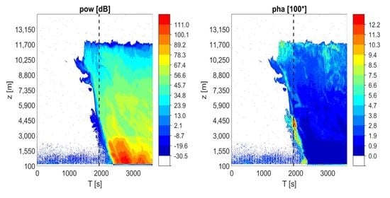
Figure 4 that the radar signal is often strongly attenuated during storms which occur in the immediate vicinity of the radar. The strong attenuation can be associated with heavy rain and other hydrometeors, which “hides” the storm (its center and its maximum intensity) to the radar, as the time evolution of the measured precipitation totals demonstrates. For instance,
Figure 4 shows that in the time interval from 2000 to 2500 s approximately, the attenuation of the radar signal caused by heavy rain was such intense that the radar measurements were available for few gates only (up to a height of 2 km roughly). To a lower extent, the same phenomenon occurred at approximately 1500 s on 1 June 2018 (
Figure 2), while the attenuation by heavy rain was not obvious from 1300 to 2000 s on 2 August 2018 (
Figure 3). Despite the strong attenuation of the signal and related low availability of radar measurements above the radar at the time of the maximum intensity of the storms on 1 June 2018 and 10 June 2019, we consider data from the initial stage and decaying stage of storms valuable for describing the behavior of the measured radar data. It should be mentioned that during other analyzed thunderstorms, we did not observe that strong attenuation of the signal.
3.2. Analysis of Pow, Pha, Powx and Phax for “Near” vs. “Far” Data
Figure 5 and
Figure 6 show distributions of measured values of pow, pha, powx and phax from all the gates for “near(1 km)” and “far” data, respectively, during the analyzed days with thunderstorms (
Table 2). It is clearly visible that the distributions are asymmetric for both the “near(1 km)” and the “far” data. Therefore, we used median and percentiles to describe the data distribution in further analyses.
Since the results might be influenced by the thickness of considered vertical layers determined by the selected number of gates, ngate, included in a layer, we clarify this influence by comparing vertical profiles for ngate=10, 15 and 20. The impact of selected ngate on the results is illustrated in
Figure 7 for pha, which depicts median values, area between 33rd and 66th percentiles and 10th and 90th percentiles (hatched curves).
Figure 7 clearly shows that the thicker the layer (i.e., larger ngate), the smoother the calculated vertical profile. On the other hand, it is also obvious that the results are similar from one ngate to another and therefore, we can consider that the results are not fundamentally dependent on the selected ngate value. Based on these results, we used ngate = 15 to illustrate further results of this study (figures hereafter).
Furthermore, the amount of processed data is, in addition to the thickness of the layer, influenced by the selected distance of the lightning discharge from the radar site, which defines the “near” data set.
Figure 8 shows the number of pha data in each vertical layer including ngate = 15 depending on the distance defining the “near” data. Note that the data decrease at higher vertical levels is the direct consequence of the attenuation of the signal, which increases with increasing distance from the radar (i.e., height in case of our vertically pointing radar) and/or because these heights are above the existing cloud tops. As far as the cross-channel quantities are concerned, their counts are much lower (not depicted) which is related to naturally lower signal received by the radar in the cross-channel.
Figure 9 and
Figure 10 compares statistical characteristics of pow, pha, powx and phax calculated for “near(0.75 km),” “near(0.5 km)” and “far” data in order to find out the features of thunderstorm and non-thunderstorm clouds occurring above the radar.
Figure 9 shows median and 10th, 33rd, 66th and 90th percentiles in the same way as
Figure 7. At the first glance, the quantity pha reaches clearly different values for thunderstorm and non-thunderstorm clouds. From a height of about 3 km, the areas between the 33rd and the 66th percentiles do not intersect. However, this is not the case for areas between the 10th and the 90th percentiles. The difference between thunderstorm and non-thunderstorm clouds is also evident for pow at altitudes of 4 to 9 km, although to a clearly smaller extent as the areas between the 33rd and the 66th percentiles do not intersect. Conversely, for powx and phax, the difference is smaller and manifests only in case of comparing medians. For powx the difference in medians is visible from 3 to 8 km, while for phax it is from 3 to 6 km.
For pow, powx and phax, the “near(0.75 km)” values are lower or comparable to those for “far” from 3 to 9 km, whereas above 10 km, the “near(0.75 km)” values gets higher than the “far” values for powx and phax. Nevertheless, we should consider that there is clearly less data in powx and phax at these heights than for other quantities. Therefore, a question arises whether these results cannot be produced by randomness of the data. This should not be the case because we obtained very similar results for “near(1 km)” data (not depicted) and for “near(0.5 km)” data (
Figure 10). Although it is clear from
Figure 10 that a smaller amount of data included in “near(0.5 km)” data causes less smooth vertical profiles showing thus more oscillations, the basic dependencies between “near(0.5 km)” and “far” data for above mentioned heights are kept. The fact that pow gives lower values for “near” data than for “far” data can be explained by lightning, which usually precedes precipitation.
3.3. Correlation Analysis of Pow, Pha, Powx and Phax for “Near” data vs. “Far” Data
To obtain the interrelationships between pow, pha, powx and phax, we performed a correlation analysis between pairs of the quantities. We calculated the correlation using the standard Pearson correlation coefficient (PC; [
28]). Since the quantities have strongly asymmetrical distributions (
Figure 5 and
Figure 6) and there are nonlinear relationships between quantities, we also performed a control calculation using the Spearman correlation coefficient (SC; [
28]). Resulting PC and SC correlations are presented in
Figure 11 and
Figure 12, respectively.
Comparison of
Figure 11 with
Figure 12 suggests that if we focus on the field structure, we can state that the resulting PC and SC do not fundamentally differ. This confirms the experience that PC can be used even if the theoretical assumptions on linearity of the relationships are not met. Based on the similarity of PC and SC (
Figure 11 and
Figure 12, respectively), we comment the PC results in the following text only as PC is easily interpretable.
It is visible in
Figure 11 and
Figure 12 that for most of the correlations of pairs between “near” and “far” data, those for “near” data are visually different from those for “far” data at various heights. To objectively evaluate the differences between the obtained correlations for “near” and “far” data we calculated the 95% confidence intervals for both PC and SC [
29]. If the intervals did not intersect then the correlations were different at the 95% level. It should be mentioned that in case of “far“ data,
Figure 11 and
Figure 12 show that the confidence intervals of 95% are very small (invisible) because of the very large size of the “far” data.
Figure 11 and
Figure 12 also confirm that the majority of the differences between correlations for “near” and “far” is statistically significant at 95% level of confidence. Comparing
Figure 11 with
Figure 12, PC values give much more points with statistically significant differences than SC values.
For all combinations of pairs in dependence on height, it is evident that the PC values for “near(0.75 km)” data differ from those for “far” data. However, it should be emphasized that PCs for “near(0.75km)” data were calculated from significantly less values as compared to PCs for “far” data. This explains the oscillating nature of “near(0.75 km)” data and the dot representation of “near(0.75 km)” data, instead of the line which we used to represent more numerous “far” data. The largest difference between PCs is for the pair pha:phax at a height of 5 to 9 km. The differences are significant at 95% confidence level with the exception of the height 6000 m for SC. This is the height where the most intense electrification of cloud usually occurs and lightning discharges originates [
30].
Another clear difference between “near(0.75 km)” and “far” data is also obvious in PCs for the pair pow:pha and pha:powx and at the same time, the mutual correlations are very similar. This corresponds to high correlations of the pair pow:powx for both the “near(0.75 km)” and the “far” data. According to SC significant differences between “near” and “far” data are from 6 km in contrast with PC where differences start at about 3 km.
The correlation structures of pow:phax and powx:phax are very similar as well as their dependence on height. Obviously, the correlation of “far” data is in some cases significantly lower than the correlation for “near(0.75km)” data. For that, it is interesting to compare these correlations expressed by PC with those expressed by SC (
Figure 11 and
Figure 12, respectively). SC correlations are significantly higher with values about 0.9 and higher. The lower PC correlations are caused by phax values, which are highly variable and can vary significantly in height. The high variability of phax together with the general nonlinearity of the relationship between pow or powx and phax are the reasons why the resulting PC values are much lower than SC values. On the other hand, very high SC values mean that the tendencies of pow or powx with phax are almost the same. For instance, if for two values of pow or powx, x and y, x <y, then for the corresponding values of phax, x´ and y´, the same inequality x´ < y´ is valid.
3.4. Estimation of Lighning Ocurrence Using the Cloud Radar Data
Since
Figure 9,
Figure 10,
Figure 11 and
Figure 12 showed that there are differences in the values of the studied quantities for “near” and “far” data, we focused on modelling the relationship between cloud radar measurements and the occurrence of lightning near the radar site using the RTE model which we verified using ROC, A (the area below ROC) and CSI (
Section 2.6). Specifically, we focused on estimating the occurrence of lightning up to 500 m, 750 m and 1 km from the radar site using the radar quantities for vertical layers including 15 gates, as in
Section 3.2 and
Section 3.3. In the following, we present results that we obtained for the distance of 750 m.
Figure 13 presents an example of ROC curves calculated at the 99 independent verification sets obtained by 99 realizations of random splitting of the data into calibration and verification data sets for a layer consisting of 15 gates with a center at about 6 km above the radar. The figure clearly shows the ability of the RTE model (its high potential) to distinguish “near” data from the “far” data. This result is also confirmed in
Figure 14, where the values of A and the values of A plus or minus the standard deviation of A are shown for all the layers having centers at different heights.
Contrary to the convincing results provided by ROC and A, verification using CSI of the yes/no RTE model outputs is less successful (
Figure 15). Mean CSI values are between 0.20 and 0.35 approximately. Significant decrease of CSI at a height above 10 km is due to the small number of data with lightning at this height and high sensitivity of the model outputs on the selected threshold. However, two points should be mentioned here. The first is that the weakest point of the RTE model is the calculation and the application of the threshold value because CSI is very sensitive to the threshold value. Note that if we used the threshold optimization on the verification file, then the CSI values would have exceeded 0.60 (not depicted). The second point is that although the CSI values are low in absolute value, according to our experience in predicting rare events such as heavy rain, the obtained CSI values can be considered quite high for such extremely rare phenomenon the lightning is.
The presented modelling can seem simple; however, there are two reasons why we intentionally applied simple modelling of the relationship between cloud radar data and lightning occurrence. The first reason is that we wanted to find out whether it is possible to model lightning occurrences using cloud radar data with reasonable results identifying thunderstorms. The second reason is that for more sophisticated models we need more data that are not at our disposal yet since thunderstorms are rare and our measurements date from 2018 only.
4. Discussion
Within this research, we encountered two problems: (i) there are few discharges detected near the radar site as compared to “far” data, (ii) there are several cases with high attenuation of the signal caused by heavy rain during a short period of time in case of strongest thunderstorms occurring in the immediate vicinity of the radar. This reduces partly the “near” data set. Nevertheless, as the heavy rain did not occur during all the analyzed thunderstorms and if it occurred, its duration was usually shorter than the period of lightning occurrence, that is, “devastating” signal attenuation was not observed. Thus, we believe that our results obtained in this study are valid, although they need to be refined as soon as we obtain larger data sets (i.e., from a longer period).
The limited number of “near” data as compared to “far” data is due to the fact that the occurrence of lightning is a very rare phenomenon at a particular place. We partly solved this problem by processing the radar data through vertical layers, consisting of several gates, instead of analyzing data per each gate. This data processing through layers has a physical justification since data of individual thunderstorms differ, the grouping of data from several gates does not disturb the results, as we have presented and at the same time it increases the robustness of the data analysis. Therefore, we believe that the obtained characteristics of the data are reliable, although the inclusion of data into the analysis from the following years will undoubtedly bring more accurate results.
Further, we did not distinguish between CC and CG discharges in our study due to the limited number of CG (5%). Therefore, our obtained results express mostly the properties of cloud radar measurements for the occurrence of CC discharges. We are aware that the localization of CC may include an error in the order of hundreds of meters which can affect our selection of “near” and “far” data based on the distance of discharges from the radar. Therefore, we used different distances for “near” data selection and separated “near” from “far” by at least 9 km. The results of the analyses for different distances defining “near” data are similar, so we believe that the inaccuracy related to possible errors in determining the location of CC discharges did not significantly affect our results.
As far as the modelling of the relationship between the cloud radar data and the occurrence of lightning in the near vicinity of the radar site concerns, it is likely going to remain problematic in future due to the fact that the proportion between “near” and “far” data will not significantly change even when the data amount will increase in future by adding additional years of measurements. Thus, the verification of the modeling will likely be limited in future as well.
Similar problem is often encountered in forecasting very rare events, for example, heavy rain. The core of the problem is that the prediction methods do not objectively predict high probabilities of the phenomenon from strongly asymmetric calibration data, where the non-occurrence of the phenomenon fundamentally prevails. As a rule, this problem is solved by considering the ratio between the calculated probability and the climatic probability of the occurrence of the phenomenon and the prediction itself is then based on the application of a profit function comparing the impacts of correct and incorrect predictions. We deliberately avoided to provide the answer whether the (lightning) phenomenon will or will not occur (i.e., identification of the event), instead we used the ROC and A analyses, which characterize the potential of separating lightning from non-lightning events based on the radar data. In addition, we also used a simple deterministic method determining the occurrence of “near” data and verified it using CSI to show what we can expect from the model in real applications.
5. Conclusions
This study analyzed and compared basic measured cloud radar quantities, namely pow, powx, pha and phax, for thunderstorm clouds producing lightning in the direct vicinity of the radar site (i.e., “near” data) and for non-thunderstorm clouds producing lightning farther from the radar site (i.e., “far” data). The analysis was performed using data from 38 days of thunderstorms which occurred in 2018 and 2019 in the region of the Milešovka observatory, where the radar is installed and which produced lightning discharges in the 20 km radius around the radar.
Our results can be summarized as follows:
The difference between “near” and “far” data is clearly manifested in the quantities of pow, pha, powx and phax. The fundamental difference is in pha. A thunderstorm cloud causes significantly higher pha values than a non-thunderstorm cloud. This is true especially for the height of 3 km and higher. Moreover, there is a clear difference between “near” and “far” data for pow, although smaller than for pha. In the case of cross-channel quantities (powx and phax), the difference between “near” and “far” data is small as compared to those in the co-channel (pha and pow).
From the correlation analysis among pow, pha, powx and phax it follows that correlation relationships are clearly different for “near” and “far” data. The biggest difference is evident for the correlations of pha vs. phax. Another finding is that pow and powx give very similar results in correlation relations, that is, the correlations of pow vs. pha and powx vs. pha as well as the correlations of pow vs. phax and powx vs. phax are very similar.
An important result is that the phase shifts, pha and phax, contain important information that is not contained in pow and powx. This is especially true for pha.
Based on differences found between the values of “near” data and those of “far” data, we tested the possibility of indicating the occurrence of lightning discharges around the radar using a RTE model on radar measurements. We found that “near” lightning events can be quite successfully distinguished from “far” lightning events using the RTE model in terms of ROC.
To answer whether a lightning discharge is close to the radar or not, the RTE model application evaluated by CSI gave values of 0.2 to 0.3 only, in dependence on the used vertical layer. Although these CSI values are low in absolute values, they can be considered quite high given the fact that lightning is a very rare phenomenon.
We are aware that the extent of data with lightning in the vicinity of the radar is limited. Therefore, we plan to extend our research using the data from next years. Further, we consider lightning measuring essential for analyses similar to ours.
Author Contributions
Z.S. and J.P. conceived the paper and discussed and interpreted the results. Z.S. developed the presented algorithms and performed most of the analyses. J.P. processed the results graphically and wrote most of the manuscript. All authors have read and agreed to the published version of the manuscript.
Funding
This research was funded by project CRREAT (reg. number: CZ.02.1.01/0.0/0.0/15_003/0000481) call number 02_15_003 of the Operational Programme Research, Development and Education and was also supported by Charles University (UNCE/HUM 018) and by project Strategy AV21 Water for Life.
Acknowledgments
We acknowledge Ondřej Fišer for consultations of the studied topic. We acknowledge Petr Pešice for administration of cloud radar data at the Milešovka observatory. We would like to express our thanks also to BLIDS for providing us with lightning data.
Conflicts of Interest
The authors declare no conflict of interest. The funders had no role in the design of the study, in the collection, analyses, or interpretation of data, in the writing of the manuscript, or in the decision to publish the results.
References
- Saunders, C.P.R.; Peck, S.L. Laboratory Studies of the Influence of the Rime Accretion Rate on Charge Transfer during Crystal/Graupel Collisions. J. Geophys. Res. Atmos. 1998, 103, 13949–13956. [Google Scholar] [CrossRef]
- Saunders, C. Charge Separation Mechanisms in Clouds. Space Sci. Rev. 2008, 137, 335–353. [Google Scholar] [CrossRef]
- Stolzenburg, M.; Rust, W.D.; Marshall, T.C. Electrical Structure in Thunderstorm Convective Regions: 2. Isolated Storms. J. Geophys. Res. Atmos. 1998, 103, 14079–14096. [Google Scholar] [CrossRef]
- MacGorman, D.R.; Biggerstaff, M.I.; Waugh, S.; Pilkey, J.T.; Uman, M.A.; Jordan, D.M.; Ngin, T.; Gamerota, W.R.; Carrie, G.; Hyland, P. Coordinated Lightning, Balloon-Borne Electric Field, and Radar Observations of Triggered Lightning Flashes in North Florida: Triggered Lightning and Storm Charge. Geophys. Res. Lett. 2015, 42, 5635–5643. [Google Scholar] [CrossRef]
- Weinheimer, A.J.; Dye, J.E.; Breed, D.W.; Spowart, M.P.; Parrish, J.L.; Hoglin, T.L.; Marshall, T.C. Simultaneous Measurements of the Charge, Size, and Shape of Hydrometeors in an Electrified Cloud. J. Geophys. Res. Atmos. 1991, 96, 20809–20829. [Google Scholar] [CrossRef]
- Winn, W.P.; Schwede, G.W.; Moore, C.B. Measurements of Electric Fields in Thunderclouds. J. Geophys. Res. 1896–1977 1974, 79, 1761–1767. [Google Scholar] [CrossRef]
- Weiss, S.A.; Rust, W.D.; MacGorman, D.R.; Bruning, E.C.; Krehbiel, P.R. Evolving Complex Electrical Structures of the STEPS 25 June 2000 Multicell Storm. Mon. Weather Rev. 2008, 136, 741–756. [Google Scholar] [CrossRef]
- Adamo, C.; Goodman, S.; Mugnai, A.; Weinman, J.A. Lightning Measurements from Satellites and Significance for Storms in the Mediterranean. In Lightning: Principles, Instruments and Applications: Review of Modern Lightning Research; Betz, H.D., Schumann, U., Laroche, P., Eds.; Springer: Dordrecht, The Netherlands, 2009; pp. 309–329. ISBN 978-1-4020-9079-0. [Google Scholar]
- Vorpahl, J.A.; Sparrow, J.G.; Ney, E.P. Satellite Observations of Lightning. Science 1970, 169, 860–862. [Google Scholar] [CrossRef]
- Saha, K.; Damase, N.P.; Banik, T.; Paul, B.; Sharma, S.; De, B.K.; Guha, A. Satellite-Based Observation of Lightning Climatology over Nepal. J. Earth Syst. Sci. 2019, 128, 221. [Google Scholar] [CrossRef]
- Sparrow, J.G.; Ney, E.P. Lightning Observations by Satellite. Nature 1971, 232, 540–541. [Google Scholar] [CrossRef]
- Labrador, L. The Detection of Lightning from Space. Weather 2017, 72, 54–59. [Google Scholar] [CrossRef]
- Makowski, J.A.; MacGorman, D.R.; Biggerstaff, M.I.; Beasley, W.H. Total Lightning Characteristics Relative to Radar and Satellite Observations of Oklahoma Mesoscale Convective Systems. Mon. Weather Rev. 2012, 141, 1593–1611. [Google Scholar] [CrossRef]
- Vonnegut, B. Orientation of Ice Crystals in the Electric Field of a Thunderstorm. Weather 1965, 20, 310–312. [Google Scholar] [CrossRef]
- Hendry, A.; McCormick, G.C. Radar Observations of the Alignment of Precipitation Particles by Electrostatic Fields in Thunderstorms. J. Geophys. Res. 1976, 81, 5353–5357. [Google Scholar] [CrossRef]
- Krehbiel, P.; Chen, T.; McCrary, S.; Rison, W.; Gray, G.; Brook, M. The Use of Dual Channel Circular-Polarization Radar Observations for Remotely Sensing Storm Electrification. Meteorol. Atmos. Phys. 1996, 59, 65–82. [Google Scholar] [CrossRef]
- Metcalf, J.I. Radar Observations of Changing Orientations of Hydrometeors in Thunderstorms. J. Appl. Meteorol. 1995, 34, 757–772. [Google Scholar] [CrossRef][Green Version]
- Biggerstaff, M.I.; Zounes, Z.; Addison Alford, A.; Carrie, G.D.; Pilkey, J.T.; Uman, M.A.; Jordan, D.M. Flash Propagation and Inferred Charge Structure Relative to Radar-observed Ice Alignment Signatures in a Small Florida Mesoscale Convective System. Geophys. Res. Lett. 2017, 44, 8027–8036. [Google Scholar] [CrossRef]
- Melnikov, V.; Zrnić, D.S.; Weber, M.E.; Fierro, A.O.; MacGorman, D.R. Electrified Cloud Areas Observed in the SHV and LDR Radar Modes. J. Atmos. Ocean. Technol. 2018, 36, 151–159. [Google Scholar] [CrossRef]
- Caylor, I.J.; Chandrasekar, V. Time-Varying Ice Crystal Orientation in Thunderstorms Observed with Multiparameter Radar. IEEE Trans. Geosci. Remote Sens. 1996, 34, 847–858. [Google Scholar] [CrossRef]
- Ryzhkov, A.V.; Zrnić, D.S. Depolarization in Ice Crystals and Its Effect on Radar Polarimetric Measurements. J. Atmos. Ocean. Technol. 2007, 24, 1256–1267. [Google Scholar] [CrossRef]
- Hubbert, J.C.; Ellis, S.M.; Chang, W.-Y.; Rutledge, S.; Dixon, M. Modeling and Interpretation of S-Band Ice Crystal Depolarization Signatures from Data Obtained by Simultaneously Transmitting Horizontally and Vertically Polarized Fields. J. Appl. Meteorol. Clim. 2014, 53, 1659–1677. [Google Scholar] [CrossRef]
- Sokol, Z.; Minářová, J.; Fišer, O. Hydrometeor Distribution and Linear Depolarization Ratio in Thunderstorms. Remote Sens. 2020, 12, 2144. [Google Scholar] [CrossRef]
- Ge, J.; Zhu, Z.; Zheng, C.; Xie, H.; Zhou, T.; Huang, J.; Fu, Q. An Improved Hydrometeor Detection Method for Millimeter-Wavelength Cloud Radar. Atmos. Chem. Phys. 2017, 17, 9035–9047. [Google Scholar] [CrossRef]
- BLIDS, der Blitz Informationsdienst von Siemens. Available online: https://new.siemens.com/global/de/produkte/services/blids.html (accessed on 10 March 2020).
- Sokol, Z.; Minářová, J.; Novák, P. Classification of Hydrometeors Using Measurements of the Ka-Band Cloud Radar Installed at the Milešovka Mountain (Central Europe). Remote Sens. 2018, 10, 1674. [Google Scholar] [CrossRef]
- Myagkov, A.; Seifert, P.; Bauer-Pfundstein, M.; Wandinger, U. Cloud Radar with Hybrid Mode towards Estimation of Shape and Orientation of Ice Crystals. Atmos. Meas. Tech. 2016, 9, 469–489. [Google Scholar] [CrossRef]
- Wilks, D.S. Statistical Methods in the Atmospheric Sciences, 4th ed.; Elsevier: Cambridge, UK, 2019; ISBN 978-0-12-815823-4. [Google Scholar]
- Press, W.H.; Teukolsky, S.A.; Vetterling, W.T.; Flannery, B.P. Numerical Recipes in C: The Art of Scientific Computing, 2nd ed.; Cambridge University Press: New York, NY, USA, 1992; ISBN 978-0-521-43108-8. [Google Scholar]
- Rakov, V.A. Fundamentals of Lightning; Cambridge University Press: Cambridge, MA, USA, 2016; ISBN 978-1-107-07223-7. [Google Scholar]
Figure 1.
Geographical location of the cloud radar MIRA35c at the Milešovka observatory on top of the Milešovka Mt. (837 m a.s.l.) in Czechia in Central Europe. Source of the topographic maps: (upper left panel) European Environment Agency (
https://www.eea.europa.eu/legal/copyright) and (upper right panel)
https://maps-for-free.com/.
Figure 2.
Time evolution of pow, pha, powx and phax (upper two rows) from 11:30 to 12:30 UTC on 1 June 2018. The x-axis shows time (T [s]), while the y-axis displays the height above the radar site (z [m]). Quantities pow and powx are in dB, whereas pha and phax are in arctan of phase degree multiplied by 100 and 1000, respectively. The dashed line shows the time of recorded lightning –as there were 6 lightning discharges registered within 1 s up to 0.75 km from the radar site, they appear as a single dashed line in the figure. The lower graph shows the 1-min precipitation totals as measured during the same period by the automated weighting rain gauge situated next to the cloud radar.
Figure 3.
Time evolution of pow, pha, powx and phax (upper two rows) from 17:00 to 18:00 UTC on 2 August 2018. The x-axis shows time (T [s]), while the y-axis displays the height above the radar site (z [m]). Quantities pow and powx are in dB, whereas pha and phax are in arctan of phase degree multiplied by 100 and 1000, respectively. The dashed lines show the time of lightning discharges recorded up to 0.75 km from the radar site. The lower graph shows the 1-min precipitation totals as measured during the same period by the automated weighting rain gauge situated next to the cloud radar.
Figure 4.
Time evolution of pow, pha, powx and phax (upper two rows) from 21:00 to 22:00 UTC on 10 June 2019. The x-axis shows time (T [s]), while the y-axis displays the height above the radar site (z [m]). Quantities pow and powx are in dB, whereas pha and phax are in arctan of phase degree multiplied by 100 and 1000, respectively. The dashed lines show the time of lightning discharges recorded up to 0.75 km from the radar site. The lower graph shows the 1-min precipitation totals as measured during the same period by the automated weighting rain gauge situated next to the cloud radar.
Figure 5.
Distribution of measured pow, pha, powx and phax for near(1 km). The x-axis of phax (right lower panel) shows accumulated number of values larger than 0.005. Both pha and phax are expressed in arctan of the phase degree.
Figure 5.
Distribution of measured pow, pha, powx and phax for near(1 km). The x-axis of phax (right lower panel) shows accumulated number of values larger than 0.005. Both pha and phax are expressed in arctan of the phase degree.
Figure 6.
Distribution of measured pow, pha, powx and phax for far. The x-axis of phax (right lower panel) shows accumulated number of values larger than 0.005. Both pha and phax are expressed in arctan of the phase degree.
Figure 6.
Distribution of measured pow, pha, powx and phax for far. The x-axis of phax (right lower panel) shows accumulated number of values larger than 0.005. Both pha and phax are expressed in arctan of the phase degree.
Figure 7.
Distribution of pha in the co-channel for (red) “near(0.75 km)” and (blue) “far” data depending on layer thickness (from the left to the right: ngate = 10, 15 and 20). Each panel shows median values (“med”), the area between 33rd and 66th percentiles (“0.66”) and the dashed lines represent 10th and 90th percentiles (“0.1” and “0.9,” respectively). The y-axis displays the height above the radar site (z [km]). The pha is expressed in arctan of the phase degree.
Figure 8.
Measured data counts (N, y-axis) for pha in individual vertical layers containing each ngate = 15. The x-axis displays the height of layer centers (z [m]) and blue columns show the number of data in “near(0.5 km).” The number of data in “near(0.75 km)” is the sum of blue and red columns, whereas the number of data in “near(1 km)” is the sum of blue, red and yellow columns.
Figure 9.
Comparison of statistical characteristics of pow, pha, powx and phax for “near(0.75 km)” and “far” data. Detailed figure caption is given in
Figure 7. Both pha and phax are depicted using 10*log10(arctan) for better representation of vertical profiles of the data.
Figure 9.
Comparison of statistical characteristics of pow, pha, powx and phax for “near(0.75 km)” and “far” data. Detailed figure caption is given in
Figure 7. Both pha and phax are depicted using 10*log10(arctan) for better representation of vertical profiles of the data.
Figure 10.
Comparison of statistical characteristics of pow, pha, powx and phax for “near(0.5 km)” and “far” data. Detailed figure caption is given in
Figure 7. Both pha and phax are depicted using 10*log10(arctan) for better representation of vertical profiles of the data.
Figure 10.
Comparison of statistical characteristics of pow, pha, powx and phax for “near(0.5 km)” and “far” data. Detailed figure caption is given in
Figure 7. Both pha and phax are depicted using 10*log10(arctan) for better representation of vertical profiles of the data.
Figure 11.
Correlations (CC) by Pearson (PC) between pairs of pow, pha, powx and phax in dependence on height (z [m]) above the radar site. Red points represent PC for “near(0.75 km)” data, while the green line indicates PC for “far” data. Horizontal lines shows 95% confidence intervals.
Figure 11.
Correlations (CC) by Pearson (PC) between pairs of pow, pha, powx and phax in dependence on height (z [m]) above the radar site. Red points represent PC for “near(0.75 km)” data, while the green line indicates PC for “far” data. Horizontal lines shows 95% confidence intervals.
Figure 12.
Correlations (CC) by Spearman (SC) between pairs of pow, pha, powx and phax in dependence on height (z [m]) above the radar site. Red points represent SC for “near(0.75 km)” data, while the green line indicates SC for “far” data. Horizontal lines shows 95% confidence intervals.
Figure 12.
Correlations (CC) by Spearman (SC) between pairs of pow, pha, powx and phax in dependence on height (z [m]) above the radar site. Red points represent SC for “near(0.75 km)” data, while the green line indicates SC for “far” data. Horizontal lines shows 95% confidence intervals.
Figure 13.
The 99 Receiver Operating Characteristic (ROC) curves calculated using random splitting of the data into calibration and verification data sets (black curves). Red line displays the mean ROC curve over 99 random realizations, whereas the blue line shows the random forecast. H on the y-axis depicts the hit rate, while F on the x-axis the false alarm rate (
Section 2.6). The results are shown for cloud radar data covering the vertical layer of 15 gates with the center at a height z = 5947 m above the radar.
Figure 14.
Calculated A, the area below ROC, in dependence on elevation above the radar site (z [m]). The figure shows mean values of A (black solid line) and mean A ± standard deviation of A (dashed lines).
Figure 14.
Calculated A, the area below ROC, in dependence on elevation above the radar site (z [m]). The figure shows mean values of A (black solid line) and mean A ± standard deviation of A (dashed lines).
Figure 15.
Calculated Critical Success Index (CSI) in dependence on elevation above the radar site (z [m]). The figure shows mean values of CSI (red solid line) and mean CSI ± standard deviation of CSI (dashed lines).
Figure 15.
Calculated Critical Success Index (CSI) in dependence on elevation above the radar site (z [m]). The figure shows mean values of CSI (red solid line) and mean CSI ± standard deviation of CSI (dashed lines).
Table 1.
Basic technical information on the cloud radar MIRA 35c situated at the Milešovka observatory.
Table 1.
Basic technical information on the cloud radar MIRA 35c situated at the Milešovka observatory.
| Technical Information | Cloud Radar MIRA 35c |
|---|
| Radar system | Doppler |
| Polarimetric radar | Yes |
| Radar band | Ka-band |
| Transmitter frequency | 35.12 GHz +/−0.1 GHz |
| Pulse repetition frequency (PRF) | 2.5–10 kHz |
| Pulse width | min. 0.1 μs |
| | max. 0.4 μs |
| Detection unambiguous velocity range | ± 10.65 m/s |
| Original measurements | Doppler spectra |
| Radar core | Magnetron |
| Antenna type | Cassegrain |
| Peak power | 2.5 kW |
| Antenna diameter | 1 m |
| Antenna gain | 48.5 dB |
| Antenna beam width | 0.6° |
Table 2.
Thunderstorms of 2018 (left panel) and 2019 (right panel) with lightning discharges registered 0–20 km from the Milešovka observatory.
Table 2.
Thunderstorms of 2018 (left panel) and 2019 (right panel) with lightning discharges registered 0–20 km from the Milešovka observatory.
| Thunderstorms in 2018 | Thunderstorms in 2019 |
|---|
| June 1 | May 20 |
| June 10 | May 25 |
| June 11 | June 6 |
| June 27 | June 10 |
| June 28 | June 12 |
| July 5 | June 20 |
| July 21 | July 21 |
| July 28 | July 29 |
| August 2 | July 31 |
| August 3 | August 2 |
| August 4 | August 3 |
| August 8 | August 4 |
| August 13 | August 7 |
| August 17 | August 11 |
| August 24 | August 12 |
| September 21 | August 27 |
| | August 29 |
| | September 1 |
| Publisher’s Note: MDPI stays neutral with regard to jurisdictional claims in published maps and institutional affiliations. |
© 2021 by the authors. Licensee MDPI, Basel, Switzerland. This article is an open access article distributed under the terms and conditions of the Creative Commons Attribution (CC BY) license (http://creativecommons.org/licenses/by/4.0/).


