A New Individual Tree Species Recognition Method Based on a Convolutional Neural Network and High-Spatial Resolution Remote Sensing Imagery

Abstract

Tree species surveys are crucial to forest resource management and can provide references for forest protection policy making. The traditional tree species survey in the field is labor-intensive and time-consuming, supporting the practical significance of remote sensing. The availability of high-resolution satellite remote sensing data enable individual tree species (ITS) recognition at low cost. In this study, the potential of the combination of such images and a convolutional neural network (CNN) to recognize ITS was explored. Firstly, individual tree crowns were delineated from a high-spatial resolution WorldView-3 (WV3) image and manually labeled as different tree species. Next, a dataset of the image subsets of the labeled individual tree crowns was built, and several CNN models were trained based on the dataset for ITS recognition. The models were then applied to the WV3 image. The results show that the distribution maps of six ITS offered an overall accuracy of 82.7% and a kappa coefficient of 0.79 based on the modified GoogLeNet, which used the multi-scale convolution kernel to extract features of the tree crown samples and was modified for small-scale samples. The ITS recognition method proposed in this study, with multi-scale individual tree crown delineation, avoids artificial tree crown delineation. Compared with the random forest (RF) and support vector machine (SVM) approaches, this method can automatically extract features and outperform RF and SVM in the classification of six tree species.

1. Introduction

Forests are among the most important terrestrial ecosystems and are essential for human development [1]. Well-managed forests provide renewable resources, protect biodiversity, maintain a stable energy cycle, and prevent soil degradation and erosion [2]. Precise tree species surveys are crucial to forest inventory and management because they provide managers with a better understanding of forest species composition, changes in forest species, quantity of forest resources, and references for the formulation and adjustment of forestry policies [3]. However, traditional survey methods are inefficient and their associated labor costs are high. Remote sensing-based methods are efficient when mapping forest types in areas with rough terrain or that are difficult to reach, and can significantly improve survey efficiency and reduce labor costs [4].

Many remote sensing-based forest classification studies have considered multi-scale remote sensing data sources. Early developments used medium-spatial resolution satellite remote sensing data, such as Landsat Thematic Mapper imagery, for regional-scale forest classification [5,6]. However, because the spatial resolution of Landsat data is relatively low, individual trees cannot be precisely mapped. Spaceborne hyperspectral data have rarely been used for individual tree species classification. Most applications of hyperspectral data to date have been airborne [7,8,9]. The high spatial resolution of airborne data meets the requirements for determining the locations of trees [10,11,12,13]; however, data acquisition costs are normally high and data processing is complex [14,15]. With the launch of IKONOS, QuickBird, GeoEye, and WorldView satellites, high-resolution optical images can be readily obtained and meet the requirements for locating individual trees. Using such high-resolution images to precisely classify tree species saves time and costs in tree distribution mapping.

Traditional classification methods, such as random forest (RF) and support vector machine (SVM), have been widely used to classify tree species [16,17,18,19]. These approaches generally require the artificial design and extraction of classification features, such as spectra, texture, and vegetation indices, in addition to linear transformations [20,21]. The classification accuracy depends largely on the rationality of the artificial feature design and selection, which is highly subjective; therefore, extensive professional knowledge is necessary.

The designed artificial features limit the information that can be used by the classifier [22]. New classification technologies are necessary to improve classification efficiency and accuracy. As a promising classification technology, convolutional neural networks (CNNs) perform well in image classification tasks [23,24]. A CNN method does not require feature engineering, and its multi-layer structure can fully use the information in the data to automatically extract abstract and higher-level features for classification. As a result, CNN methods tend to result in accurate classifications.

In recent years, CNNs have shown satisfactory results when applied to tree species classification [25]. CNNs have been applied to classify three-dimensional point clouds of trees [26,27], airborne hyperspectral data [28,29], and high-resolution data combined with LiDAR data [30]. These studies were almost all based on airborne imaging systems and multiple data sources, which are characterized by high data acquisition costs and complex data processing, preventing their wide application. To date, CNNs have rarely been applied to recognize individual tree species (ITS) from a single satellite data source. A method is needed for using satellite data to classify ITS for mapping forest tree species with a low data acquisition cost.

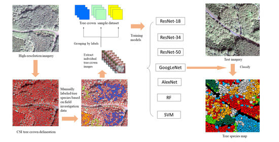
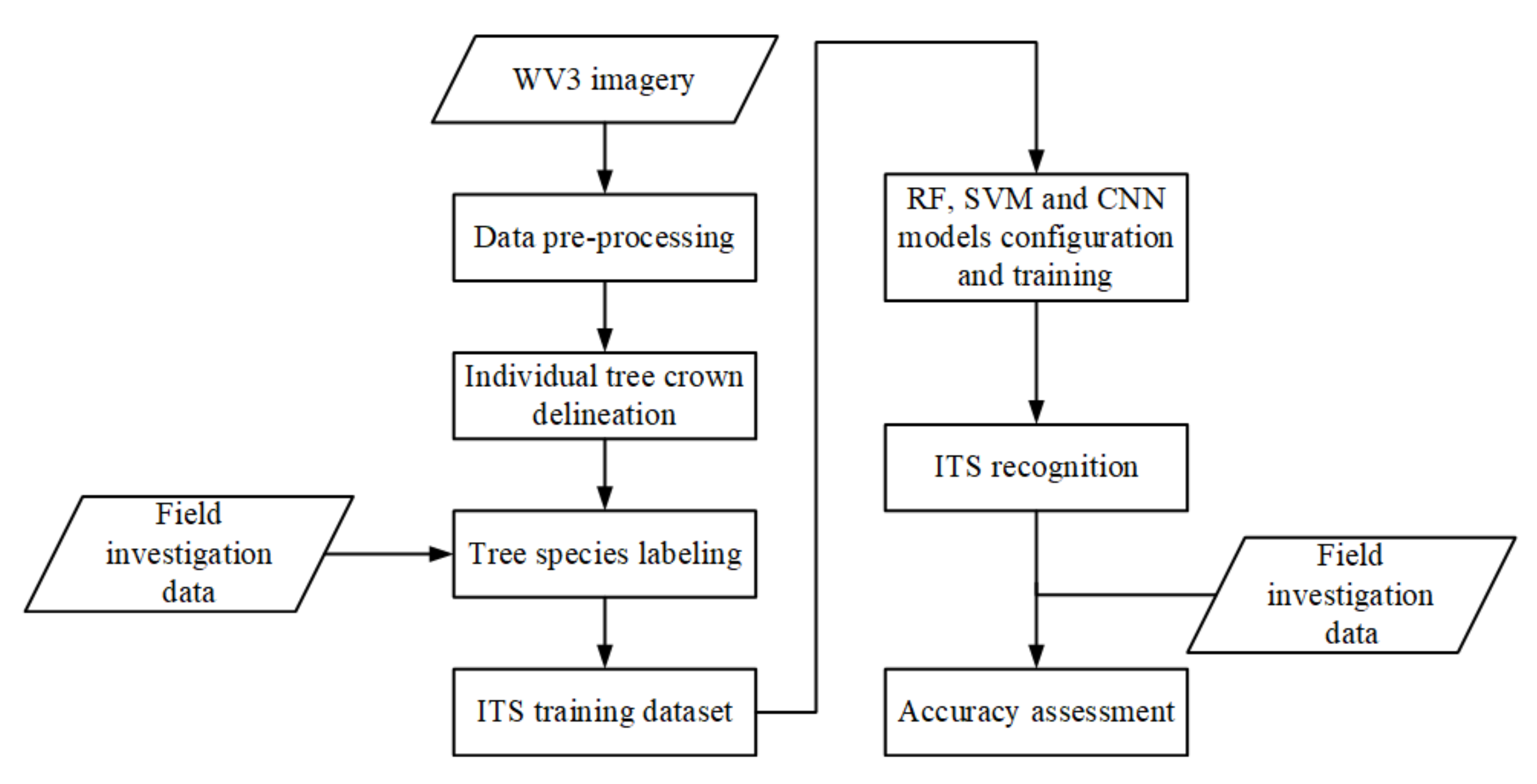
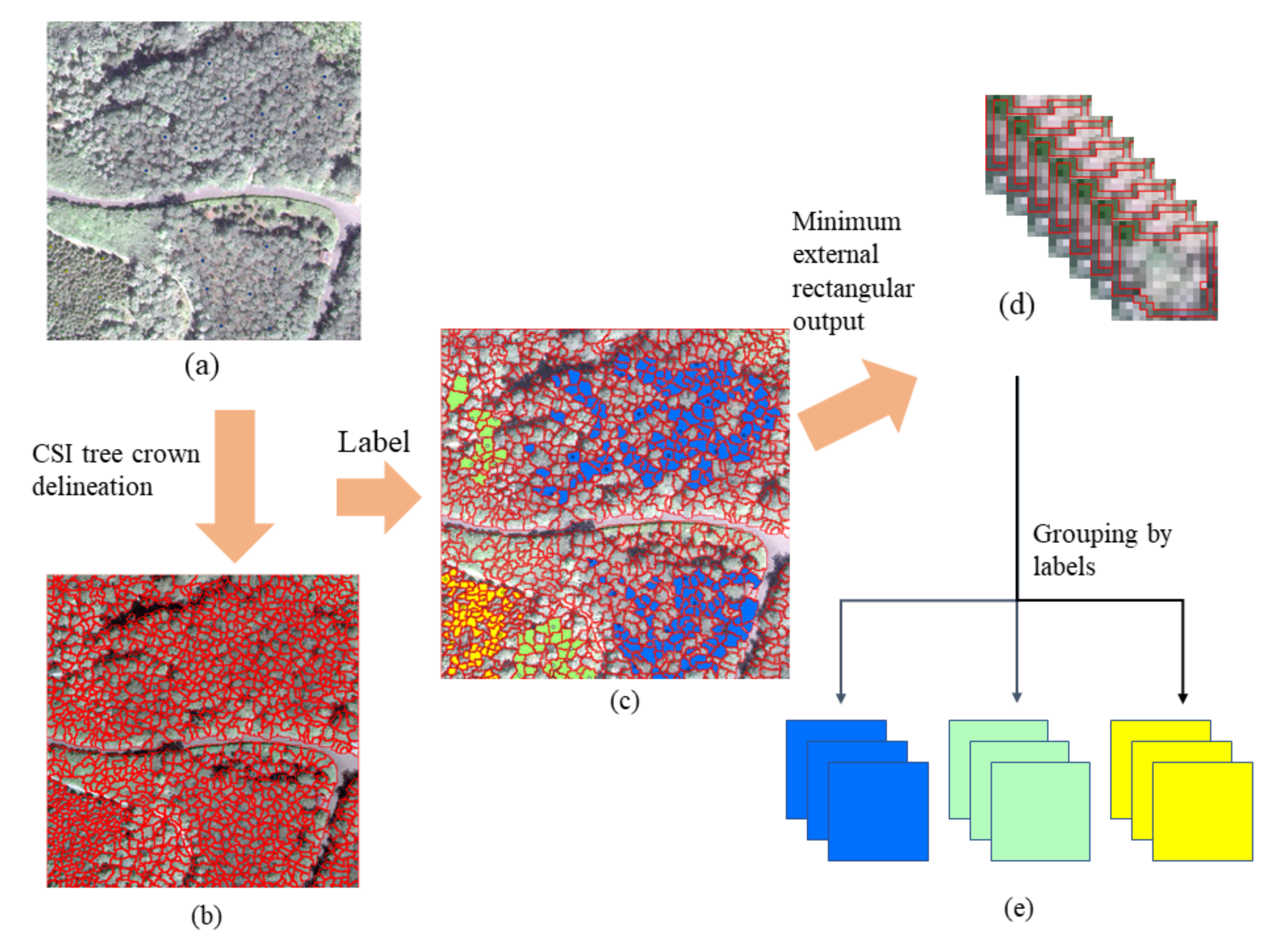
In this study, we explored the combination of high-resolution satellite remote sensing imagery and CNNs to recognize ITS. A CNN-based multi-scale ITS recognition (CMSIR) method was developed to improve the automation and accuracy of ITS mapping. In the CMSIR method, a tree crown delineation approach is used to quickly build an individual tree crown training dataset, and several popular CNN models are employed to automatically extract classification features and recognize ITS from a high-resolution satellite image. The multi-scale characteristic of different tree species was considered in tree crown delineation and ITS recognition.

2. Materials and Methodologies

2.1. Study Area

The study area (Figure 1) is located in the Olympic Forest Park (116°22′29″E–116°23′43″E, 40°0′30″–40°1′11″N), Chaoyang District, Beijing, China. The total area of the park is approximate 100 ha and the vegetation coverage rate is 95.6% [31,32]. The forests inside were manually planted and arranged in rows, clusters, and groups with a large number of single tree species. The study area was suitable for constructing a standard sample dataset due to the similarity of trees within specific zones, including tree height, size, and species. Shrubs were planted on the periphery of the arbor forest to act as a natural fence to separate roads from trees. Artificial buildings are sparsely distributed in the forest, and occupy a small portion of the area and have little impact on the forest.

2.2. Data

2.2.1. Field Investigation Data

A field investigation of tree species in the study area was carried out in October 2018, for several days. Trees in the study area were manually planted in a monoculture scheme; thus, many zones in the study area had consistent tree species. The boundaries of zones with consistent tree species were marked on images. The orange boundaries in Figure 2 are an example of the marked zones. On the first day, we entered each marked zone and located 3–5 GPS points with a Trimble^® Geo7X global positioning system (GPS) handheld device (Trimble Inc., Sunnyvale, CA, USA). The points in Figure 2 show the located GPS points in the marked zones. The position accuracy was improved by taking the mean value of the measured real-time position 10 times. Simultaneously, the tree species of each marked zone was identified by expert experience and recorded together with the located GPS points. After the first day’s investigation, GPS points were overlaid on the image, and we found that the points were almost all located in the marked zones. Therefore, the GPS was accurate enough to locate the marked zones. The dominant tree species in the study area were determined based on the first day’s investigation result, and the investigation was continued over the next several days to obtain more samples. In addition, understory trees in forests cannot be observed via remote sensing images and therefore were not sampled. All of the samples were distributed as shown in Figure 3; the dominant tree species included 175 ash (Fraxinus chinensis Roxb.), 132 poplar (Populus tomentosa), 128 cypress (Sabina chinensis), 127 pagoda (Sophora japonica), 127 willow (Salix babylonica L.), and 110 pine (Pinus L.). The field investigation data supported the manual labeling of tree crowns and the interpretation of tree species.

2.2.2. Remote Sensing Data and Pre-Processing

A cloud-free subset of a high-resolution WorldView-3 (WV3) Beijing scene acquired on 4 September 2014 was used in this study. The acquisition date of the image was within the fully developed season, which provides good conditions for the classification of tree species.

The dataset consisted of four 3145 × 3145 multispectral bands with 1.6 m spatial resolution, including blue (0.450–0.510 μm), green (0.510–0.580 μm), red (0.630–0.690 μm), and near-infrared (NIR; 0.770–0.895 μm) bands, and a corresponding 12,580 × 12,580 panchromatic band (0.450–0.800 μm) with 0.4 m spatial resolution. Although the WV3 sensor provides 16 multispectral bands, the image collected over the study area only had four standard bands. A digital elevation model (DEM) was used to orthorectify the panchromatic and multispectral images, which were fused using the Gram–Schmidt method in the ENVI 5.3 (L3Harris Geospatial, Broomfield, CO, USA) package to obtain a four-band fused multispectral image with a cell size of 0.4 m. The pre-processed image showed good overall geometric precision with less than 1 pixel offset compared with the control points in the field investigation.

2.3. Methodologies

As shown in Figure 4, the flowchart of the CMSIR method proposed in this study includes seven steps: (1) data pre-processing; (2) individual tree crown (ITC) delineation using the crown slices from imagery (CSI) tree crown delineation algorithm [33]; (3) tree species labeling based on field investigation; (4) ITS training dataset construction; (5) RF, SVM, and CNN model configuration and training; (6) ITS recognition using RF, SVM, and CNN; and (7) accuracy assessment with field investigation data.

2.3.1. Training Dataset

The training samples were collected from five typical regions in the study area (blue rectangles in Figure 3). These five regions were selected because they included patches of consistent tree species, so it was easy to label tree species. The test sample collection region (yellow rectangle in Figure 3) was used to construct the test dataset to evaluate the performance of the trained models and generate the tree species classification maps. The test region included all tree species in the training dataset and few non-vegetation features and no grassland, so interference was reduced. In addition, we separated the training data from test data to ensure independence of the training and testing samples.

A training dataset with labeled trees was needed to train classification models, so a process was designed to quickly create an ITC training dataset. First, segmentation maps obtained from the CSI tree crown delineation algorithm were overlaid on the image. Second, tree species were labeled based on the field investigation data and manual interpretation. We judged the quality of the delineation during manual labeling: tree crowns without clearly visible appearances were discarded, and only the well-delineated tree crowns were labeled. Thus, the error caused by the CSI delineation was reduced. Third, the minimum outer cut rectangle of each labeled tree was taken to obtain the ITC slice images. Finally, the sliced images with the same labels were grouped into the same category. Figure 5 shows the training dataset construction process.

CSI Tree Crown Delineation Algorithm

To avoid manual delineation of tree crowns, the CSI tree crown delineation algorithm [33] was used to extract ITCs. This algorithm was developed for multi-scale ITC delineation from high-resolution optical imagery, and can effectively reduce image over-segmentation and provide fine tree crown maps. It consists of 5 steps: (1) The three-dimensional (3D) radiometric shape of a tree crown is considered as a half-ellipsoid. The half-ellipsoid can be horizontally sliced into a series of slices from top to bottom, and the slices represent multiple tree crown levels of different scales. The morphological opening operations are used to measure dominant sizes of tree crowns. (2) Multiple Gaussian filters are used to generate multi-scale representations of the forest image from the multiple tree crown levels obtained in step 1. (3) The watershed segmentation method [34] is used on the multi-scale representations of the forest image obtained in step 2 to generate multi-scale segmentation maps. The multi-scale segmentation maps represent the target forest’s multi-scale tree crown sizes. (4) The boundaries of segments generated in step 3 are adjusted using the filtered image at a coarse scale based on the original image at the dominant size. (5) The multi-scale segmentation maps obtained in step 4 are integrated to generate the final tree crown map. In this study, the method of visual evaluation was adopted. Adjusting the parameters in the algorithm, the match between the delineation lines and the real tree crowns was visually assessed to obtain the most accurate delineation map [35].

Data Augmentation

Increasing the number of sample images can improve the generalization ability of the model. Due to the limited number of available field samples, data augmentation was used to increase the number of sample images. Data augmentation applies transformations on labeled images to increase the number of samples. Commonly used transformations include rotation, translation, random scaling, cropping, and flipping. Because the scale of each sample image was small, random scaling and clipping methods were not applied. Each labeled image was rotated by 90°, 180°, and 270°, and was flipped horizontally and vertically. After data augmentation, the number of samples increased by a factor of five. The number of training samples for each species is shown in

Table 1. The statistics of the training samples.

Tree Species	Number of Training Samples	Number of Training Samples After Data Augmentation	Image
Pine	324	1944
Cypress	227	1362
Poplar	430	2580
Ash	491	2946
Pagoda	486	2916
Willow	538	3228
Total	2496	14,976

, and the total number of training samples after augmentation was 14,976. Each image had the four R, G, B, and NIR channels.

Features Extraction

Feature extraction was performed with RF and SVM methods to classify tree crowns. Spectra, texture, and shape features were considered for extraction; they are described in

Table 2. Features used in this study.

Group	Feature Name	Description
Spectra	Mean	The average value of all pixels contained in the object in band n
	Variance	The variance value of all pixels contained in the object in band n
	Maximum	The maximum value of all pixels contained in the object in band n
	Minimum	The minimum value of all pixels contained in the object in band n
Texture	Angular second moment (ASM)	Measures the number of repeated pairs
	Contrast	Measures the local contrast
	Entropy	Measures the randomness of a gray-level distribution
	Correlation	Measures the correlation between pairs of pixels
Shapes	Width	Width of an object
	Height	Height of an object
	Compactness	Indicates compactness of an object
	Boundary length	The sum of pixels of an object boundary.

. Texture and shape features were considered in this study because crowns of different tree species have various structures, shapes, and canopy densities [28,30].

2.3.2. CNN Model Configuration

CNN models were used to classify tree species in this study. CNN models were inspired by biological neural perception mechanisms, with the relationships between layers being similar to those used by the human vision system [36]. When processing multi-dimensional images, CNN models can automatically extract features that are beneficial to image interpretation and processing. CNN models have been widely used in image classification tasks [37], and have become a popular research topic in the field of recognition and classification [38,39]. A common CNN model is comprised of an input layer, stacks of convolution and pooling layers, a fully connected layer, and an output layer [40]. Inspired by the effects of CNN models on visual image classification, we considered several CNN models that have demonstrated excellent performance in image classification in recent years. ImageNet Large Scale Vision Recognition Challenge (ILSVRC) is a worldwide influential platform used to evaluate computer vision and artificial intelligence algorithms. Since 2010, several CNN-based deep learning models have won the image classification challenge, significantly contributing to the development of CNN models. We selected some models that won the ILSVRC to classify ITC images: AlexNet, GoogLeNet, and ResNet. Other winning network models are not listed because their structures are too complex to handle small-scale images.

AlexNet

AlexNet [23] was the first breakthrough CNN architecture and won the 2012 ILSVRC. AlexNet firstly applies rectified linear units (ReLU) as the activation function to successfully accelerate model convergence. The dropout function is used to prevent overfitting, and the addition of a local response normalization (LRN) layer increases its generalization ability. AlexNet has been widely used due to its relatively simple network structure and shallow depth. The AlexNet model was originally used to classify the 224 × 224 × 3 ImageNet dataset. For the dataset in this study, the convolution kernel and the output of the network are both large, so the scale of the network needs to be reduced.

We modified AlexNet as follows: First, the input layer was altered from 227 × 227 × 3 to 15 × 15 × 4. Secondly, the first convolution layer was reduced from 11 × 11 to 5 × 5 to prevent underfitting problems caused by an excessively large local receptive field. Next, all of the strides of the pooling layers were decreased from 2 × 2 to 1 × 1 to avoid a feature map that was too small. Then, the number of convolution filters was decreased by 6 to 7, and the output of the fully connected layer was reduced from 4096 to 140 or 70 to prevent overfitting. The modified AlexNet model structure is shown in

Table 3. Modified AlexNet model structure. ReLU, rectified linear units.

Layer	Input Size	Output Size	Parameter
Conv1	15 × 15 × 4	8 × 8 × 16	kernel 5 × 5, filter 16, stride 2
Max pooling1	8 × 8 × 16	6 × 6 × 16	pool size 3 × 3, stride 1
Conv2	6 × 6 × 16	6 × 6 × 48	kernel 5 × 5, filter 48, stride 1
Max pooling2	6 × 6 × 48	4 × 4 × 48	pool size 3 × 3, stride 1
Conv4	4 × 4 × 48	4 × 4 × 54	kernel 3 × 3, filter 54, stride 1
Conv5	4 × 4 × 54	4 × 4 × 54	kernel 3 × 3, filter 54, stride 1
Conv6	4 × 4 × 54	4 × 4 × 36	kernel 3 × 3, filter 36, stride 1
Max pooling3	4 × 4 × 36	2 × 2 × 36	pool size 3 × 3, stride 1
Fully connected1	2 × 2 × 36	140	ReLU, dropout 0.5
Fully connected2	140	70	ReLU, dropout 0.5
Output	70	6	Softmax

.

GoogLeNet

GoogLeNet [41] was established by Szegedy’s team, who won the title of ILSVRC classification task champion in 2014. The original GoogLeNet model was used to classify the ImageNet image set at 224 × 224 × 3. Thus, it was necessary to modify the network to adapt to the small-scale samples in this study.

The modified GoogLeNet consisted of one input layer, one convolutional layer, eight inception modules, two downsample modules, one pooling layer, and the classification layer (

Table 4. Modified GoogLeNet model structure.

Layer Name	Input Size	Output Size	Parameter
Convolutional	15 × 15 × 4	15 × 15 × 96	kernel 3 × 3, filter 96, stride 1
Inception module 1a	15 × 15 × 96	15 × 15 × 64	I: filter 32, II: filter 32
Inception module 1b	15 × 15 × 64	15 × 15 × 80	I: filter 32, II: filter 48
Downsampling module1	15 × 15 × 80	7 × 7 × 160	III: filter 80, IV: maxpooling
Inception module 2a	7 × 7 × 160	7 × 7 × 160	I: filter 112, II: filter 48
Inception module 2b	7 × 7 × 160	7 × 7 × 160	I: filter 96, II: filter 64
Inception module 2c	7 × 7 × 160	7 × 7 × 160	I: filter 80, II: filter 80
Inception module 2d	7 × 7 × 160	7 × 7 × 144	I: filter 48, II: filter 96
Downsampling module2	7 × 7 × 144	3 × 3 × 240	III: filter 96, IV: maxpooling
Inception module 3a	3 × 3 × 240	3 × 3 × 336	I: filter 176, II: filter 160
Inception module 3b	3 × 3 × 336	3 × 3 × 336	I: filter 176, II: filter 160
Average Pooling	3 × 3 × 336	1 × 1 × 336	pool size 3 × 3
Fully connected	1 × 1 × 336	336	dropout 0.5
Output	336	6	Softmax

). The fully connected layer was replaced by the global average pooling layer to greatly reduce the number of parameters. Therefore, there were far fewer training parameters for the modified GoogLeNet, and the memory allocation was significantly reduced.

In the inception module, the output of the previous layer is passed to two parallel paths, called path I and path II. The two paths contain a convolution layer, a normalization layer, and an activation layer. The convolutional layer filter size in path I is 1 and 3 in path II. The inception module learns the 1 × 1 and 3 × 3 filters (which are computed in parallel) and concatenates the resulting feature maps along the channel dimensions. In general, this process allows the network to learn local features with small convolutions and abstract features with large convolutions.

Table 5. Inception module 1a structure.

Path I	Path II
conv_1: kernel 1 × 1, filter 32, stride 1	conv_2: kernel 3 × 3, filter 32, stride 1
Batch normalization	Batch normalization
ReLU	ReLU
Concatenation

lists the structure of the inception module 1a, which has 32 filters in the convolution layer and uses batch normalization in the normalization layer and ReLU in the activation layer. The other inception modules differ only in the number of filters. In the downsampling module, the output of the previous layer is passed into two parallel paths: path III and path IV. Path III is composed of a convolution layer, a normalization layer, and an activation layer, where the convolution layer filter size is 3, the stride is 2, and the downsampling module1 has 80 filters. Path III uses batch normalization in the normalization layer and ReLU in the activation layer. Path IV is a maxpooling layer with a pooling size of 3 × 3 and a stride of 2.

Table 6. Downsampling module1 structure.

Path III	Path IV
conv: kernel 3 × 3, filter 80, stride 2	Maxpooling size 3 × 3, stride 2
Batch normalization
ReLU
Concatenation

shows the structure of the downsampling module 1. The only difference in the downsampling module 2 is that it has 96 filters in the convolution layer. The output feature maps of paths III and IV are concatenated along the channel dimensions.

ResNet

ResNet [42] was proposed to solve the problem of gradient disappearance after increasing the network depth and won first place at the 2015 ILSVRC. This model divides the output of the neurons into H(x) and F(x) in a certain layer and establishes a shortcut between convolution layers to form a residual unit (Figure 6). H(x) is the expected output after the input x passes through the convolution layers. The residual F(x) is the difference between the expected output H(x) and the input x, so F(x) = H(x) − x. The shortcut passes the input information to the subsequent layer to protect the integrity of the information and converts the learning object into residuals. The network only needs to learn the residuals F(x) rather than the complete output, and does not increase the network parameters or the computational complexity, but can greatly reduce the difficulty of network optimization and simplify the learning objectives. ResNet maintains training accuracy when the network depth is increased. Because our training image size was generally smaller than 20 × 20 pixels, the feature map would shrink after pooling. ResNet has only two pooling layers but has a deep network structure, making it suitable as a feature extractor for small images. The structures of the 18-, 34-, and 50-layer ResNet models are shown in

Table 7. ResNet model structures.

Layer Name	18-Layer	34-Layer	50-Layer
Conv1	kernel 5 × 5, filter 32, stride 2
Max pooling	Pool size 3 × 3, stride 2
Conv2_x	$\left[\begin{array}{c}3\times 3, 64\\ 3\times 3, 64\end{array}\right]$× 2	$\left[\begin{array}{c}3\times 3, 64\\ 3\times 3, 64\end{array}\right]$× 3	$\left[\begin{array}{c}1\times 1, 64\\ 3\times 3, 64\\ 1\times 1, 256\end{array}\right]$× 3
Conv3_x	$\left[\begin{array}{c}3\times 3, 128\\ 3\times 3, 128\end{array}\right]$× 2	$\left[\begin{array}{c}3\times 3, 128\\ 3\times 3, 128\end{array}\right]$× 4	$\left[\begin{array}{c}1\times 1, 128\\ 3\times 3, 128\\ 1\times 1, 512\end{array}\right]$× 4
Conv4_x	$\left[\begin{array}{c}3\times 3, 256\\ 3\times 3, 256\end{array}\right]$× 2	$\left[\begin{array}{c}3\times 3, 256\\ 3\times 3, 256\end{array}\right]$× 6	$\left[\begin{array}{c}1\times 1, 256\\ 3\times 3, 256\\ 1\times 1, 1024\end{array}\right]$× 6
Conv5_x	$\left[\begin{array}{c}3\times 3, 512\\ 3\times 3, 512\end{array}\right]$× 2	$\left[\begin{array}{c}3\times 3, 512\\ 3\times 3, 512\end{array}\right]$× 3	$\left[\begin{array}{c}1\times 1, 512\\ 3\times 3, 512\\ 1\times 1, 2048\end{array}\right]$× 3
Average pooling	Pool size 2 × 2, stride 1
Output	Softmax

. We changed the parameters of conv1 to make the network suitable for small sample training, and the other structures are consistent with those in He [42].

2.3.3. Model Training

The training dataset was split randomly into training (75%) and validation (25%) samples. Each image was resized to 15 × 15 to ensure all of the sizes of images input into network were the same. The batch size was set to 60, which was the total number of training images used to train the model at each update. The deep learning platform was based on Tensorflow1.6 and Keras2.1.

A maximum of 500 epochs was set and an early stopping approach was used to avoid overfitting. The loss was calculated based on the validation samples after the operation of each epoch. If the loss did not decrease after 10 epochs, the training was stopped and the weights that provided the best validation accuracy were saved. Models in the actual training process usually converged within 150 epochs. The initial learning rate was set to 10⁻⁴. The learning rate decay was set to ensure that the network could automatically reduce the learning rate based on the loss situation. The learning rate would decay when the loss was not reduced after the operation of five epochs. The learning rate factor for each reduction was 5 × 10⁻³, with a lower limit of the learning rate of 5 × 10⁻⁶.

Several models were trained by adjusting the parameters during the training process. The CNN model that had the highest validation accuracy was saved for later testing.

To verify the classification performance of CNN, two machine learning classifiers were tested for comparison: RF and SVM. These are widely used to classify tree species because they can accurately handle high-dimensional data [30]. RF is an ensemble learning algorithm that trains a classifier composed of multiple decision trees through a bagging strategy [43]. The training samples of each decision tree are obtained by random sampling, and the classification result is the majority classification result of all decision trees. During the test, we found that when the number of trees exceeded 500, the accuracy did not increase significantly. To save computing time, the number of trees was set to 500. SVM creates a model that is based on a user-defined kernel function and transforms the data into classes. Then, an optimal hyperplane that maximizes the margin distance between classes can be found [44]. The radial basis function was used as the kernel function, with a grid search method [45] to determine optimal classifier parameters in the study.

2.3.4. Accuracy Assessment

The test image in Figure 7 was used to assess the generalization error of the models. The test image was cropped by the yellow rectangle in Figure 3, and was completely independent of training samples. The separation of testing from training data is important to evaluate the classification results. Each tree crown in the test image was extracted using the CSI tree crown delineation algorithm, and the minimum outer cut rectangle of each crown was extracted as a test sample. The test samples were predicted with the CNN models as described in Section 2.3.2. Simultaneously, RF and SVM were used for comparison. The label and location of each test sample were combined to generate tree species classification maps by assigning the predicted labels to the delineated tree crowns. The test points were based on the field investigation and were used as true values to calculate the following indexes: (a) confusion matrices; (b) producer accuracy (PA); (c) user accuracy (UA); (d) average accuracy (AA); (e) overall accuracy (OA); (f) kappa coefficient.

3. Results

Table 8. Confusion matrix and statistical measures of RF, SVM, AlexNet, GoogLeNet, and ResNet for individual tree species classification. PA, producer accuracy; UA, user accuracy; AA, average accuracy; OA, overall accuracy.

RF
Classified as	Pine	Cypress	Poplar	Ash	Pagoda	Willow
Pine	2	0	0	0	0	0
Cypress	12	13	4	0	2	0
Poplar	1	1	14	0	4	1
Ash	0	0	0	18	0	13
Pagoda	0	1	4	4	4	10
Willow	0	0	0	6	8	5
PA (%)	13.3	86.7	63.6	64.3	22.2	17.2
UA (%)	100.0	41.9	66.7	58.1	17.4	26.3
AA (%)	56.7	64.3	65.2	61.2	19.8	21.8
OA (%)	44.1			Kappa	0.32
SVM
Classified as	Pine	Cypress	Poplar	Ash	Pagoda	Willow
Pine	9	1	5	0	2	1
Cypress	1	14	0	0	0	0
Poplar	5	0	14	0	1	0
Ash	0	0	0	11	0	2
Pagoda	0	0	3	17	14	26
Willow	0	0	0	0	1	0
PA (%)	60.0	93.3	63.6	39.3	77.8	0.0
UA (%)	50.0	93.3	70.0	84.6	23.3	0.0
AA (%)	55.0	93.3	66.8	62.0	50.6	0.0
OA (%)	48.8			Kappa	0.40
AlexNet
Classified as	Pine	Cypress	Poplar	Ash	Pagoda	Willow
Pine	0	0	0	0	0	0
Cypress	3	7	0	0	0	0
Poplar	10	7	20	0	4	0
Ash	0	0	0	26	2	21
Pagoda	1	0	2	0	5	0
Willow	1	1	0	2	7	8
PA (%)	0.0	46.7	90.9	92.9	27.8	27.6
UA (%)	0.0	70.0	48.8	53.1	62.5	42.1
AA (%)	0.0	58.3	69.9	73.0	45.1	34.9
OA (%)	52.0			Kappa	0.41
GoogLeNet
Classified as	Pine	Cypress	Poplar	Ash	Pagoda	Willow
Pine	13	2	1	0	0	0
Cypress	0	13	0	0	0	0
Poplar	0	0	17	0	0	2
Ash	0	0	0	22	1	3
Pagoda	1	0	4	0	16	0
Willow	1	0	0	6	1	24
PA (%)	86.7	86.7	77.3	78.6	88.9	82.8
UA (%)	81.3	100.0	89.5	84.6	76.2	75.0
AA (%)	84.0	93.3	83.4	81.6	82.5	78.9
OA (%)	82.7			Kappa	0.79
ResNet-18
Classified as	Pine	Cypress	Poplar	Ash	Pagoda Tree	Willow
Pine	13	3	1	0	0	0
Cypress	0	12	0	0	0	0
Poplar	0	0	16	0	0	1
Ash	0	0	0	16	4	4
Pagoda	0	0	5	0	14	0
Willow	2	0	0	12	0	24
PA (%)	86.7	80.0	72.7	57.1	77.8	82.8
UA (%)	76.5	100.0	94.1	66.7	73.7	63.2
AA (%)	81.6	90.0	83.4	61.9	75.7	73.0
OA (%)	74.8			Kappa	0.69
ResNet-34
Classified as	Pine	Cypress	Poplar	Ash	Pagoda	Willow
Pine	13	3	2	0	0	0
Cypress	0	12	0	0	0	0
Poplar	0	0	15	0	1	2
Ash	0	0	0	13	2	4
Pagoda	1	0	5	0	14	0
Willow	1	0	0	15	1	23
PA (%)	86.7	80.0	68.2	46.4	77.8	79.3
UA (%)	72.2	100.0	83.3	68.4	70.0	57.5
AA (%)	79.5	90.0	75.8	57.4	73.9	68.4
OA (%)	70.9			Kappa	0.65
ResNet-50
Classified as	Pine	Cypress	Poplar	Ash	Pagoda	Willow
Pine	12	3	1	0	0	0
Cypress	0	12	0	0	0	0
Poplar	0	0	13	0	0	1
Ash	0	0	0	16	5	2
Pagoda	2	0	8	1	12	0
Willow	1	0	0	11	1	26
PA (%)	80.0	80.0	59.1	57.1	66.7	89.7
UA (%)	75.0	100.0	92.9	69.6	52.2	66.7
AA (%)	77.5	90.0	76.0	63.4	59.4	78.2
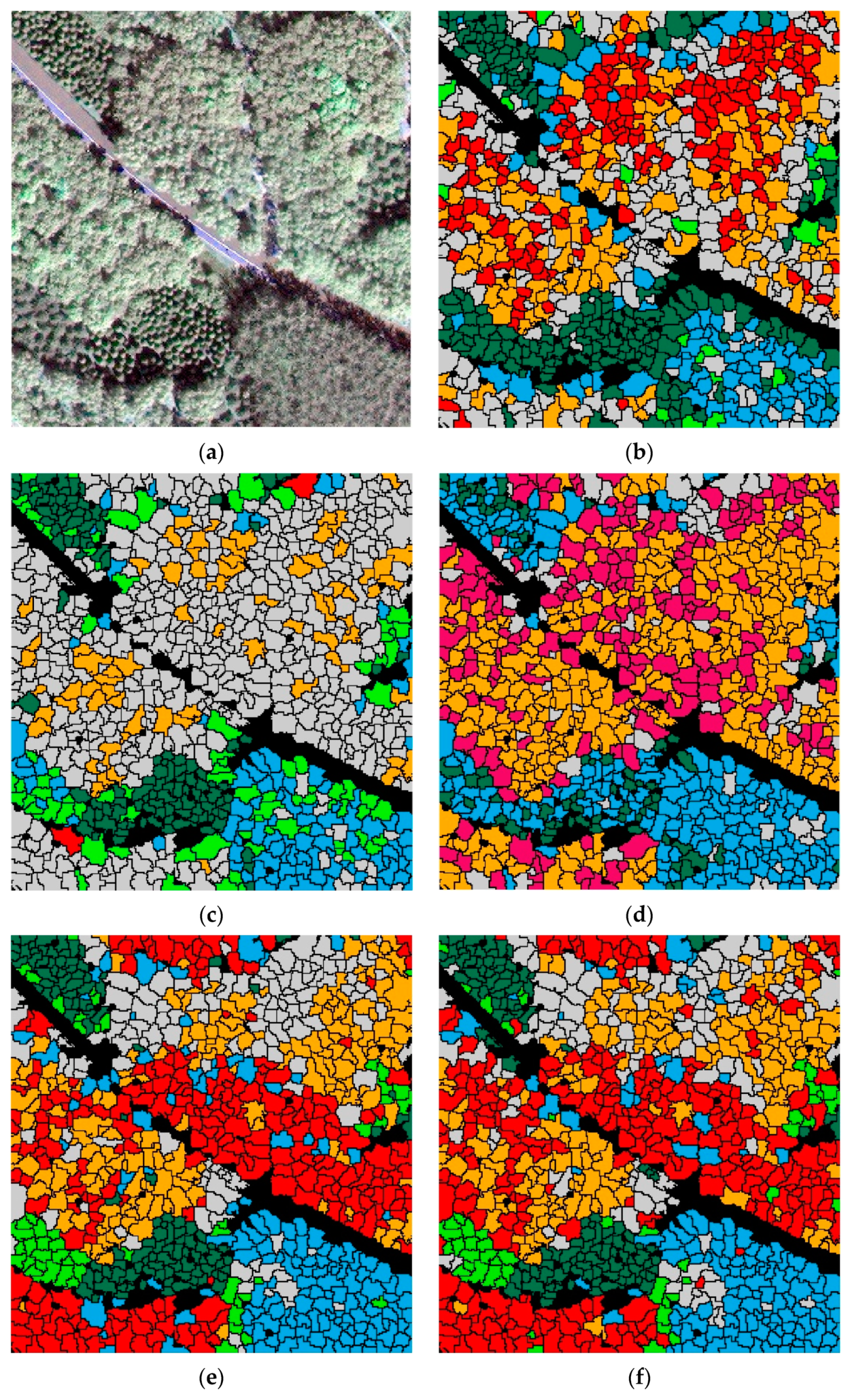
OA (%)	71.7			Kappa	0.65

shows confusion matrices and statistical measures of RF, SVM, AlexNet, GoogLeNet, and ResNet for ITS classification.

Table 9. Classification accuracies for six tree species using RF, SVM, AlexNet, GoogLeNet, and ResNet. All values except for kappa coefficient, are percentages.

Species	RF	SVM	AlexNet	GoogLeNet	ResNet-18	ResNet-34	ResNet-50
Pine	56.7	55.0	0.0	84.0	81.6	79.5	77.5
Cypress	64.3	93.3	58.3	93.3	90.0	90.0	90.0
Poplar	65.2	66.8	69.9	83.4	83.4	75.8	76.0
Ash	61.2	62.0	73.0	81.6	61.9	57.4	63.4
Pagoda	19.8	50.6	45.1	82.5	75.7	73.9	59.4
Willow	21.8	0.0	34.9	78.9	73.0	68.4	78.2
Kappa	0.32	0.40	0.41	0.79	0.69	0.65	0.65
OA	44.1	48.8	52.0	82.7	74.8	70.9	71.7

shows the classification accuracies and kappa coefficients for six species based on different models. For CNN models, GoogLeNet achieved the best OA (82.7%) with the highest kappa coefficient (0.79), and was the only model that achieved an OA over 80%. It was followed by ResNet-18 (74.8%), ResNet-50 (71.7%), ResNet-34 (70.9%), and AlexNet, which achieved the lowest OA (52.0%) and kappa coefficient (0.41). GoogLeNet achieved the highest OA for each tree species, with almost all exceeding 80%. AlexNet misclassified almost all pines as poplars, and its classification accuracy for cypress (58.3%), pagoda (45.1%), and willow (34.9%) was about 30% lower than those of GoogLeNet and ResNet. All ResNet misclassified many ashes into willows; its classification accuracy for ash was significantly lower (20%) than that of GoogLeNet. ResNet-18 outperformed ResNet-34 and ResNet-50 of OA by 3.9% and 3.1%, respectively (74.8% > 70.9% > 71.7%).

Compared with RF and SVM, the OA of GoogLeNet (82.7%) was significantly higher than that of RF (44.1%) and SVM (48.8%); even AlexNet had higher OA (52.0%) than RF (44.1%) and SVM (48.8%). Likewise, CNN models all achieved higher kappa coefficients than RF (0.32) and SVM (0.40). RF classified almost all pines as cypresses, making pines almost invisible in the classification map. The classification accuracy of RF for pine, cypress, poplar, and ash ranged from 20% to 30%, which is much lower than that of GoogLeNet. The classification accuracies of RF for pagoda and willow were only about 20%. SVM classified almost all willows as pagodas, making willows almost invisible in the classification map. The classification accuracy of SVM for pine, poplar, ash, and pagoda ranged from 20% to 30%, much lower than that achieved by GoogLeNet.

Figure 8 shows the ITS maps predicted by RF, SVM, and CNN. RF misclassified almost all pine as cypress. SVM did not separate willow from ash and pagoda. AlexNet classified many pines as poplars or cypresses.

The CSI tree crown delineation produced inevitable errors due to under- and over-segmentation, which are common problems in tree crown delineations [35], especially when only two-dimensional information is used. Some non-crown segments produced by the under- and over-segmentation affected the classification map and reduced classification accuracies. Some tree crowns were misclassified, especially on both sides of the road and the edge of the image, because some non-crown pixels were included in test samples when taking the minimum outer cut rectangles, which changed the classification features of the test samples.

4. Discussion

4.1. Classification Results of Different CNN Models

GoogLeNet achieved the best classification accuracy, followed by ResNet. In addition, AlexNet achieved the lowest accuracy. AlexNet is sequential, in which the output of the previous layer is directly input into the next layer. In contrast, GoogLeNet and ResNet have micro-architecture modules that enable networks to learn faster and more efficiently with increasing depth. The micro-architectural building blocks are stacked together with traditional layers, such as convolution and pool layers, to form the macro-architectures. The results showed that the micro-architecture can improve the classification accuracy. GoogLeNet achieved the highest classification accuracy (82.7%) and similar accuracies for each tree species, which were all higher than 80%, because GoogLeNet uses multi-scale convolution filters to extract features. Coniferous and deciduous tree crowns have different sizes; multi-scale features can be extracted by multi-scale convolution filters in GoogLeNet. The findings suggest that GoogLeNet, with a multi-scale feature extractor, is well-suited for tree species classification. As a comparison, Hartling et al. [30] used WV2/3 and LiDAR data and DenseNet to classify eight tree species; the maximum OA was 82.6%, which is similar to the accuracy in this study. However, the accuracy of different tree species varied greatly. Cypress and oak can be accurately classified with accuracy above 90%, but ash classification accuracy is only 60%. The GoogLeNet used in our study can provide similar accuracies, which were all higher than 80% for each tree species. Sothe et al. [28] used hyperspectral and photogrammetric data for classifying fourteen tree species in a rain forest; the forest environment was more complicated compared to our study area. The best result was achieved by the CNN with an OA of 84.4%, which outperformed SVM and RF. Fricker et al. [29] used high-spatial resolution airborne hyperspectral imagery to identify tree species in a mixed-conifer forest and the OA reached 87% for the hyperspectral CNN model. However, the study area in Fricker et al. [29] was located in the Southern Sierra Nevada Mountains, CA, USA, so the distribution of trees across an elevation gradient could be analyzed and dead trees were recognized as an individual category. Our study area was located in a park with flat terrain, where trees were manually planted and taken care of by gardeners. In addition, compared with natural forests with abundant and disorganized species, the distribution of trees in our study had a certain pattern that was easy to classify. Thus, higher accuracies would be expected in the manually planted forest.

4.2. Classification Results of Different Tree Species

The ResNet classification results showed that the classification accuracy of different tree species varied widely. The classification accuracies of conifers (pine, cypress) and poplar were above 80%, whereas the classification accuracies of ash, pagoda, and willow were lower than 70%. The test image shows that the texture and shape of the pine, cypress, and poplar are unique and show obvious differences. However, the differences among ash, pagoda, and willow are not obvious. The unique crown shape of cypress creates clear boundaries among trees. Furthermore, accurate segmentation of the crown means that ITC images have large inter-class differences and small intra-class differences, which is conducive to feature extraction and classification. Therefore, the classification accuracy of cypress was highest, reaching 90%. Liu et al. [46] also concluded that the classification accuracies of conifers, which have obvious crown structures, are higher. Differences in the crowns among ash, pagoda, and willow are small; thus, the features extracted by the network are similar, which results in the misclassification of ash, pagoda, and willow. Liu et al. [46] concluded that if two species have similar crown structures, they are prone to misclassification, a finding that is supported by the results of our study. Deciduous tree crowns are dense and the gaps between crowns are small, which complicates delineating deciduous tree crowns. Inaccurate tree crown delineation would reduce differences between tree species and reduce classification accuracy.

4.3. Comparison with Other Machine Learning Models

Spectra, texture, and shape features were extracted for tree species classification based on machine learning methods such as RF and SVM; these features and classifiers have been widely used in other research related to tree species classification [28,30,47]. The methods based on RF or SVM require manual feature extraction, which is usually complicated and requires researchers to design a large number of features based on professional knowledge and experience. Conversely, the methods based on CNN use multi-layer neural networks to abstract from low- to high-level features, avoiding manual feature extraction, thus simplifying the process of feature extraction [22,48]. The results of this study also showed that the CNN obtained higher OA than RF or SVM. The OA of GoogLeNet for six species reached 82.7%, whereas those of RF and SVM were 44.09% and 48.82%, respectively. GoogLeNet significantly outperformed RF and SVM. Many studies compared the classification effects of CNN, RF, and SVM. For example, Hartling [30] showed that DenseNet, RF, and SVM for the classification of eight tree species had an OA of 82.6%, 51.8%, and 52%, respectively, with CNN showing higher accuracy. Sothe et al. [28] used CNN to achieve 22% and 26% higher OA than SVM and RF for hyperspectral data, respectively. The outstanding performance of CNN is due to its ability to enhance the texture, shape, and spatial information in images, and to use that information to detect generic structures in other images [49].

5. Conclusions

Based on practical application requirements, the CMSIR method focuses on two key issues in ITS recognition: fast and accurate construction of a training sample dataset and ITS classification methods. We proposed a method to construct ITC training samples suitable for CNN models. This method combines a multi-scale ITC delineation method, manual labeling of tree species, and sample enhancement techniques to build a training sample dataset. The CSI tree crown delineation algorithm was used to automatically describe tree crowns, which avoided manual sketching.

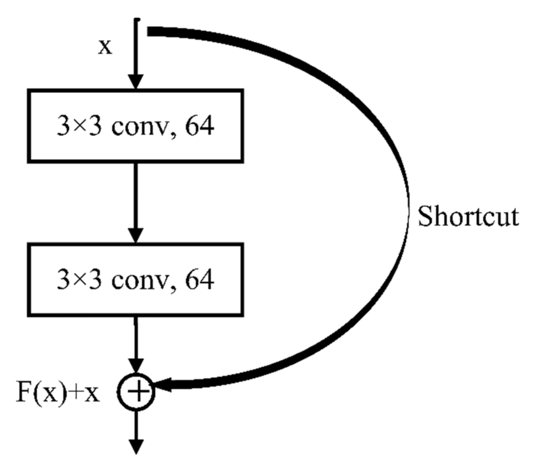
A method for ITS classification was explored using different CNN methods and high-resolution satellite remote sensing imagery. The data source was readily obtained and was low in cost and wide in scope. The CNN used in this study avoids manual feature extraction and its structures are relatively common, easy to build, and have a low training difficulty and fast training speed. GoogLeNet, which achieved the highest OA, can use multi-scale convolution filters to extract features in multi-scale tree crowns. The classification accuracies for tree crowns in different scales were very high (greater than 80%). Compared with other commonly used machine learning models, such as RF and SVM, the CNN models do not require manual feature extraction and achieve higher OA.

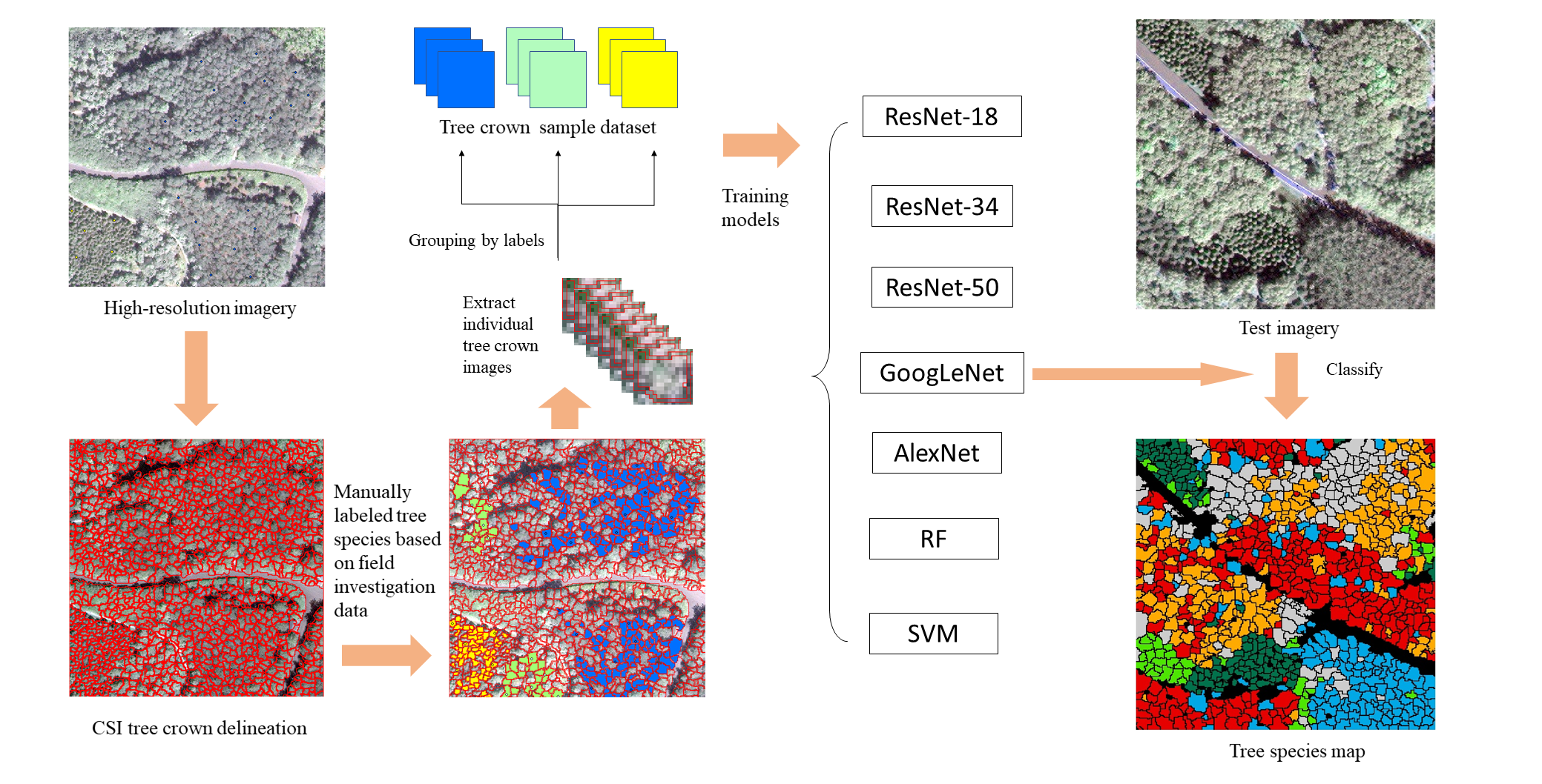
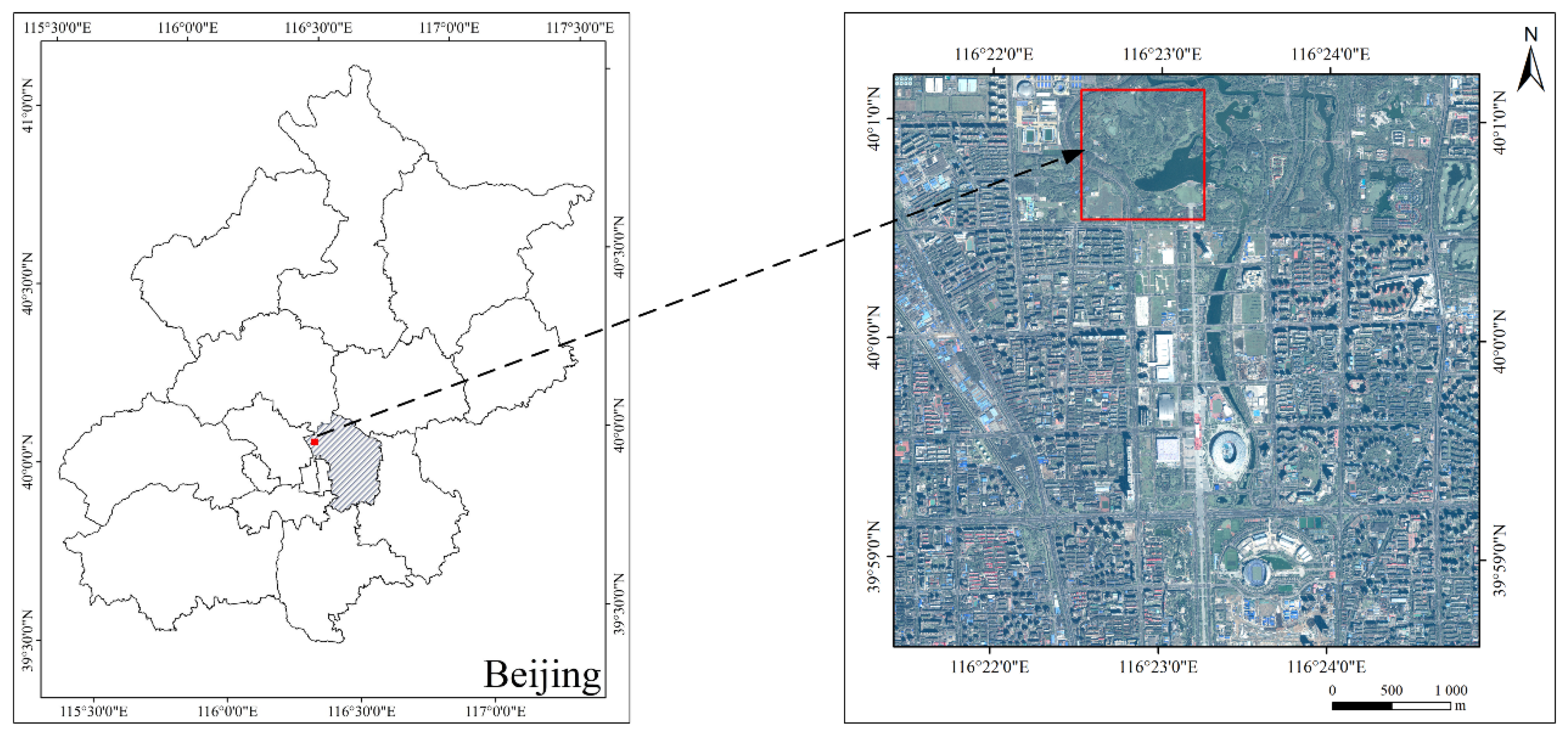
Our study area was located in a park, where trees were manually planted and pruned regularly by gardeners. The distribution of trees had a certain pattern. The crowns of the same trees were similar in size. There were intervals between the crowns, which made it easier to delineate the crowns. Thus, we expected higher accuracies in the manually planted forest. The CMSIR method could be improved in future research in the following ways: (1) Natural forests have a larger number of tree species and the distribution of tree species is more random. The tree crown delineation significantly influences the accuracy of the subsequent classification. Researchers need to effectively delineate tree crowns, especially in dense natural forests. (2) We used some classic CNN models, which were originally used for the ILSVRC dataset. Compared with ILSVRC images, tree crown images have smaller scales and multiple bands. Therefore, a network model suitable for small-scale and multiband images should be constructed for ITS classification.

References

1. Zaki, N.A.M.; Abd Latif, Z. Carbon sinks and tropical forest biomass estimation: A review on role of remote sensing in aboveground-biomass modelling. Geocarto Int. 2017, 32, 701–716. [Google Scholar] [CrossRef]
2. Bravo, F.; LeMay, V.; Jandl, R. Managing Forest Ecosystems: The Challenge of Climate Change, 2nd ed.; Springer: New York, NY, USA, 2008; pp. 3–15. [Google Scholar]
3. Kangas, A.; Maltamo, M. Forest Inventory: Methodology and Applications; Springer: Dordrecht, The Netherlands, 2006; Volume 10, p. 368. [Google Scholar]
4. Liu, Y.A.; Gong, W.S.; Hu, X.Y.; Gong, J.Y. Forest type identification with random forest using Sentinel-1A, Sentinel-2A, multi-temporal Landsat-8 and DEM data. Remote Sens. 2018, 10, 946. [Google Scholar] [CrossRef] [Green Version]
5. Wulder, M.A.; Hall, R.J.; Coops, N.C.; Franklin, S.E. High spatial resolution remotely sensed data for ecosystem characterization. Bioscience 2004, 54, 511–521. [Google Scholar] [CrossRef] [Green Version]
6. Ke, Y.; Quackenbush, L.J.; Im, J. Synergistic use of QuickBird multispectral imagery and LIDAR data for object-based forest species classification. Remote Sens. Environ. 2010, 114, 1141–1154. [Google Scholar] [CrossRef]
7. Chen, E.; Li, Z.; Tan, B.; Liang, Y.; Zhang, Z. Validation of statistic based forest types classification methods using hyperspectral data. Scientia Silvae Sinicae. 2007, 43, 84–89. [Google Scholar]
8. Ghosh, A.; Fassnacht, F.E.; Joshi, P.K.; Koch, B. A framework for mapping tree species combining hyperspectral and LiDAR data: Role of selected classifiers and sensor across three spatial scales. Int. J. Appl. Earth Obs. Geoinf. 2014, 26, 49–63. [Google Scholar] [CrossRef]
9. Yu, L.; Yu, Y.; Liu, X.; Du, Y.; Zhang, H. Tree species classification with hyperspectral image. J. Northeast For. Univ. 2016, 44, 40–43, 57. [Google Scholar]
10. Reitberger, J.; Krzystek, P.; Stilla, U. Analysis of full waveform LIDAR data for the classification of deciduous and coniferous trees. Int. J. Remote Sens. 2008, 29, 1407–1431. [Google Scholar] [CrossRef]
11. Suratno, A.; Seielstad, C.; Queen, L. Tree species identification in mixed coniferous forest using airborne laser scanning. ISPRS J. Photogramm. Remote Sens. 2009, 64, 683–693. [Google Scholar] [CrossRef]
12. Yu, X.; Litkey, P.; Hyyppa, J.; Holopainen, M.; Vastaranta, M. Assessment of low density full-waveform airborne laser scanning for individual tree detection and tree species classification. Forests 2014, 5, 1011–1031. [Google Scholar] [CrossRef] [Green Version]
13. Hovi, A.; Korhonen, L.; Vauhkonen, J.; Korpela, I. LiDAR waveform features for tree species classification and their sensitivity to tree- and acquisition related parameters. Remote Sens. Environ. 2016, 173, 224–237. [Google Scholar] [CrossRef]
14. Fassnacht, F.E.; Latifi, H.; Sterenczak, K.; Modzelewska, A.; Lefsky, M.; Waser, L.T.; Straub, C.; Ghosh, A. Review of studies on tree species classification from remotely sensed data. Remote Sens. Environ. 2016, 186, 64–87. [Google Scholar] [CrossRef]
15. Immitzer, M.; Atzberger, C.; Koukal, T. Tree species classification with random forest using very high spatial resolution 8-band WorldView-2 satellite data. Remote Sens. 2012, 4, 2661–2693. [Google Scholar] [CrossRef] [Green Version]
16. Somers, B.; Asner, G.P. Tree species mapping in tropical forests using multi-temporal imaging spectroscopy: Wavelength adaptive spectral mixture analysis. Int. J. Appl. Earth Obs. Geoinf. 2014, 31, 57–66. [Google Scholar] [CrossRef]
17. Lee, J.; Cai, X.; Lellmann, J.; Dalponte, M.; Malhi, Y.; Butt, N.; Morecroft, M.; Schonlieb, C.-B.; Coomes, D.A. Individual Tree Species Classification From Airborne Multisensor Imagery Using Robust PCA. IEEE J. Sel. Top. Appl. Earth Obs. Remote Sens. 2016, 9, 2554–2567. [Google Scholar] [CrossRef] [Green Version]
18. Le Louarn, M.; Clergeau, P.; Briche, E.; Deschamps-Cottin, M. “Kill Two Birds with One Stone”: Urban Tree Species Classification Using Bi-Temporal Pleiades Images to Study Nesting Preferences of an Invasive Bird. Remote Sens. 2017, 9, 916. [Google Scholar] [CrossRef] [Green Version]
19. Mishra, N.B.; Mainali, K.P.; Shrestha, B.B.; Radenz, J.; Karki, D. Species-level vegetation mapping in a Himalayan treeline ecotone using unmanned aerial system (UAS) imagery. ISPRS Int. Geo Inf. 2018, 7, 445. [Google Scholar] [CrossRef] [Green Version]
20. Moisen, G.G.; Freeman, E.A.; Blackard, J.A.; Frescino, T.S.; Zimmermann, N.E.; Edwards, T.C., Jr. Predicting tree species presence and basal area in Utah: A comparison of stochastic gradient boosting, generalized additive models, and tree-based methods. Ecol. Model. 2006, 199, 176–187. [Google Scholar] [CrossRef]
21. Franklin, S.E.; Ahmed, O.S. Deciduous tree species classification using object-based analysis and machine learning with unmanned aerial vehicle multispectral data. Int. J. Remote Sens. 2018, 39, 5236–5245. [Google Scholar] [CrossRef]
22. Zhang, L.; Zhang, L.; Du, B. Deep Learning for Remote Sensing Data: A technical tutorial on the state of the art. IEEE Geosci. Remote Sens. Mag. 2016, 4, 22–40. [Google Scholar] [CrossRef]
23. Krizhevsky, A.; Sutskever, I.; Hinton, G.E. Imagenet classification with deep convolutional neural networks. In Proceedings of the Twenty-Sixth Annual Conference on Neural Information Processing Systems, Lake Tahoe, NV, USA, 3–8 December 2012; pp. 1097–1105. [Google Scholar]
24. Liu, B.; Yu, X.C.; Yu, A.Z.; Wan, G. Deep convolutional recurrent neural network with transfer learning for hyperspectral image classification. J. Appl. Remote Sens. 2018, 12, 17. [Google Scholar] [CrossRef]
25. Kattenborn, T.; Leitloff, J.; Schiefer, F.; Hinz, S. Review on Convolutional Neural Networks (CNN) in vegetation remote sensing. ISPRS J. Photogramm. Remote Sens. 2021, 173, 24–49. [Google Scholar] [CrossRef]
26. Guan, H.; Yu, Y.; Ji, Z.; Li, J.; Zhang, Q. Deep learning-based tree classification using mobile LiDAR data. Remote Sens. Lett. 2015, 6, 864–873. [Google Scholar] [CrossRef]
27. Zou, X.H.; Cheng, M.; Wang, C.; Xia, Y.; Li, J. Tree Classification in Complex Forest Point Clouds Based on Deep Learning. IEEE Geosci. Remote Sens. Lett. 2017, 14, 2360–2364. [Google Scholar] [CrossRef]
28. Sothe, C.; De Almeida, C.M.; Schimalski, M.B.; La Rosa, L.E.C.; Castro, J.D.B.; Feitosa, R.Q.; Dalponte, M.; Lima, C.L.; Liesenberg, V.; Miyoshi, G.T.; et al. Comparative performance of convolutional neural network, weighted and conventional support vector machine and random forest for classifying tree species using hyperspectral and photogrammetric data. GISci. Remote Sens. 2020, 57, 369–394. [Google Scholar] [CrossRef]
29. Fricker, G.A.; Ventura, J.D.; Wolf, J.A.; North, M.P.; Davis, F.W.; Franklin, J. A Convolutional Neural Network Classifier Identifies Tree Species in Mixed-Conifer Forest from Hyperspectral Imagery. Remote Sens. 2019, 11, 2326. [Google Scholar] [CrossRef] [Green Version]
30. Hartling, S.; Sagan, V.; Sidike, P.; Maimaitijiang, M.; Carron, J. Urban Tree Species Classification Using a WorldView-2/3 and LiDAR Data Fusion Approach and Deep Learning. Sensors 2019, 19, 1284. [Google Scholar] [CrossRef] [Green Version]
31. Hu, M.M. Preliminary Study on Plant Landscape and Eco-Efficiency of Beijing Olympic Forest Park. Master’s Thesis, Beijing Forestry University, Beijing, China, 2009. (In Chinese). [Google Scholar]
32. Qin, C. Cooling and Humidifying Effects and Driving Mechanisms of Beijing Olympic Forest Park in Summer. Ph.D. Thesis, Beijing Forestry University, Beijing, China, 2010. (In Chinese). [Google Scholar]
33. Jing, L.; Hu, B.; Noland, T.; Li, J. An individual tree crown delineation method based on multi-scale segmentation of imagery. ISPRS J. Photogramm. Remote Sens. 2012, 70, 88–98. [Google Scholar] [CrossRef]
34. Chen, Q.; Baldocchi, D.; Gong, P.; Kelly, M. Isolating individual trees in savanna woodland using small footprint LIDAR data. Photogramm. Eng. Remote Sensing 2006, 72, 923–932. [Google Scholar] [CrossRef] [Green Version]
35. Qiu, L.; Jing, L.; Hu, B.; Li, H.; Tang, Y. A New Individual Tree Crown Delineation Method for High Resolution Multispectral Imagery. Remote Sens. 2020, 12, 585. [Google Scholar] [CrossRef] [Green Version]
36. Alom, M.Z.; Taha, T.M.; Yakopcic, C.; Westberg, S.; Sidike, P.; Nasrin, M.S.; Hasan, M.; Van Essen, B.C.; Awwal, A.A.S.; Asari, V.K. A State-of-the-Art Survey on Deep Learning Theory and Architectures. Electronics 2019, 8, 292. [Google Scholar] [CrossRef] [Green Version]
37. LeCun, Y.; Bengio, Y.; Hinton, G. Deep learning. Nature 2015, 521, 436–444. [Google Scholar] [CrossRef] [PubMed]
38. Dang, Y.; Zhang, J.; Deng, K.; Zhao, Y.; Yu, F. Study on the Evaluation of Land Cover Classification using Remote Sensing Images Based on AlexNet. J. Geo-Inf. Sci. 2017, 19, 1530–1537. [Google Scholar]
39. Liu, Y.; Huang, X.; Li, H.; Liu, Z.; Cheng, C.; Wang, X. Extraction of Irregular Solid Waste in Rural based on Convolutional Neural Network and Conditional Random Field Method. J. Geo-Inf. Sci. 2019, 21, 259–268. [Google Scholar]
40. Vedaldi, A.; Lenc, K. MatConvNet: Convolutional neural networks for MATLAB. In Proceedings of the 23rd ACM International Conference on Multimedia, Brisbane, Australia, 26–30 October 2015. [Google Scholar]
41. Szegedy, C.; Liu, W.; Jia, Y.; Sermanet, P.; Reed, S.; Anguelov, D.; Erhan, D.; Vanhoucke, V.; Rabinovich, A. Going Deeper with Convolutions. In Proceedings of the IEEE Conference on Computer Vision and Pattern Recognition, Columbus, OH, USA, 24–27 June 2014; pp. 1–9. [Google Scholar]
42. He, K.; Zhang, X.; Ren, S.; Sun, J. Deep Residual Learning for Image Recognition. In Proceedings of the IEEE Conference on Computer Vision and Pattern Recognition, Boston, MA, USA, 7–12 June 2015; pp. 770–778. [Google Scholar]
43. Gislason, P.; Benediktsson, J.A.; Sveinsson, J.M. Random forests for land cover classification. Pattern. Recogn. Lett. 2006, 27, 294–300. [Google Scholar] [CrossRef]
44. Cortes, C.; Vapnik, V. Support-vector networks. Mach. Learn. 1995, 20, 273–297. [Google Scholar] [CrossRef]
45. Chang, C.-C.; Lin, C.-J. LIBSVM: A Library for Support Vector Machines. ACM Trans. Intell. Syst. Technol. 2011, 2. [Google Scholar] [CrossRef]
46. Liu, L.; Coops, N.C.; Aven, N.W.; Pang, Y. Mapping urban tree species using integrated airborne hyperspectral and LiDAR remote sensing data. Remote Sens. Environ. 2017, 200, 170–182. [Google Scholar] [CrossRef]
47. Ferreira, M.P.; Zortea, M.; Zanotta, D.C.; Shimabukuro, Y.E.; de Souza Filho, C.R. Mapping tree species in tropical seasonal semi-deciduous forests with hyperspectral and multispectral data. Remote Sens. Environ. 2016, 179, 66–78. [Google Scholar] [CrossRef]
48. Gao, Q.; Lim, S.; Jia, X. Hyperspectral Image Classification Using Convolutional Neural Networks and Multiple Feature Learning. Remote Sens. 2018, 10, 299. [Google Scholar] [CrossRef] [Green Version]
49. Sylvain, J.D.; Drolet, G.; Brown, N. Mapping dead forest cover using a deep convolutional neural network and digital aerial photography. ISPRS J. Photogramm. Remote Sens. 2019, 156, 14–26. [Google Scholar] [CrossRef]
Figure 1. Location of the research area.
Remotesensing 13 00479 g001
Figure 2. Example of marked investigation zones and located global positioning system (GPS) points.
Remotesensing 13 00479 g002
Figure 3. Locations of tree species samples (red dots) identified during the field investigation. Training sample collection regions (blue rectangles) and the test sample collection region (yellow rectangle).
Remotesensing 13 00479 g003
Figure 4. The technical flowchart of the convolutional neural network (CNN)-based multi-scale individual tree species (ITS) recognition (CMSIR) method. RF, random forest; SVM, support vector machine.
Remotesensing 13 00479 g004
Figure 5. Schematic diagram of the training dataset construction. (a) Image of training sample collection region, (b) crown slices from imagery (CSI) algorithm-generated individual tree crown (ITC) map, (c) tree species labeled, (d) ITC slice images, (e) ITC training dataset.
Remotesensing 13 00479 g005
Figure 6. Building residual block. F(x), residual; x, input.
Remotesensing 13 00479 g006
Figure 7. The test image used for the accuracy assessment.
Remotesensing 13 00479 g007
Figure 8. (a) The test image. Individual tree species map obtained by (b) RF, (c) SVM, (d) AlexNet, (e) GoogLeNet, (f) ResNet-18, (g) ResNet-34, and (h) ResNet-50.
Remotesensing 13 00479 g008aRemotesensing 13 00479 g008b