Mapping Essential Urban Land Use Categories in Beijing with a Fast Area of Interest (AOI)-Based Method

Abstract

Urban land use mapping is critical to understanding human activities in space. The first national mapping result of essential urban land use categories of China (EULUC-China) was released in 2019. However, the overall accuracies in some of the plain cities such as Beijing, Chengdu, and Zhengzhou were lower than 50% because many parcel-based mapping units are large with mixed land uses. To address this shortcoming, we proposed an area of interest (AOI)-based mapping approach, choosing Beijing as our study area. The mapping process includes two major steps. First, grids with different sizes (i.e., 300 m, 200 m, and 100 m) were derived from original land parcels to obtain classification units with a suitable size. Then, features within these grids were extracted from Sentinel-2 spectral data, point of interest (POI), and Tencent Easygo crowdedness data. These features were classified using a random forest (RF) classifier with AOI data, resulting in a 10-category map of EULUC. Second, we superimposed the AOIs layer on classified units to do some rectification and offer more details at the building scale. The overall accuracy of the AOI layer reached 98%, and the overall accuracy of the mapping results reached 77%. This study provides a fast method for accurate geographic sample collection, which substantially reduces the amount of fieldwork for sample collection and improves the classification accuracy compared to previous EULUC mapping. The detailed urban land use map could offer more support for urban planning and environmental policymaking.

1. Introduction

Urban areas are the places where humankind has dramatically transformed the surface, affecting the Earth’s biochemical cycles and climate from local to global scales. With rapid urbanization, urban areas are playing a more significant role in changing the process, distribution, and patterns of hydrology, climate, biodiversity, economic development, and human well-being on Earth. For example, the impervious cover is increased in urban areas, which funnels accumulated pollutants from buildings, roadways, and parking lots into streams, thus changing hydrology. The concentration of transportation and industry in urban centers means that cities are point sources of CO₂ and other greenhouse gases, affecting Earth’s climate. Urbanization usually reduces both species richness and evenness for most biotic communities within cities as well as native species diversity at regional and global scales. The unprecedented rates of urban population growth over the past century have occurred on <3% of the global terrestrial surface, yet the impact has been global, with 78% of carbon emissions, 60% of residential water use, and 76% of wood used for industrial purposes attributed to cities. Urban dwellers depend on the productive and assimilative capacities of ecosystems well beyond their city boundaries—“ecological footprints” tens to hundreds of times the area occupied by a city—to produce the flows of energy, material goods, and nonmaterial services (including waste absorption) that sustain human well-being and quality of life [1,2]. To better support the development of adaptation planning to respond to climate change, it is critical to acquire high-quality (accurate and high resolution) urban land-use data. However, it is difficult to meet the requirements of efficiency and accuracy of land-use mapping through traditional mapping methods of visual interpretation and mathematical statistics in rapidly urbanizing areas [3].

Powerful in self-adaptive capability, machine-learning methods are popularly applied in land-use classification. Random Forests, support vector machines, and artificial neural networks have made a great contribution to land-cover/land-use classification [4,5,6,7,8,9,10,11]. The support vector machine (SVM) is applied to reduce the execution time of storing and processing hyperspectral images [11]. Simple/multiple linear regression, random forest (RF), and support vector regression (SVR) were used to estimate canopy nitrogen weight of maize leaves, and the results showed that both machine learning models performed much better than linear regression [4]. Multisource remote sensing imagery was used to obtain a wetland species map using an RF classifier [9]. Sentinel-2 and airborne imagery were also used for the mapping of citrus and other crops in highly fragmented areas [10].

However, land-use classification differs from land-cover classification due to the fact that land cover focuses on natural attributes, while land use focuses more on social attributes. Although there are some similarities between these two attributes, in urban areas, more emphasis is placed on land-use patterns and conditions. Due to the spectral and textural similarity between different categories of urban land use, remote sensing imagery cannot adequately reveal the socioeconomic attributes resulting from human activities. The complexity of socioeconomic attributes makes urban land-use classification more challenging.

With the development of big data, many new data sources were introduced into the land-use classification field. Mobile phone record data, floating car data, social media data, and other big data have shown their importance in land-use classification [3,12,13,14,15,16,17,18]. Although the inclusion of socioeconomic data can improve the accuracy of land-use classification, studies combining image data and multiple-source Internet open data to classify urban land use are relatively rare, and few studies have been conducted in large cities. Urban areas in Europe were predicted by means of Open Street Map (OSM) with artificial neural networks and genetic algorithms [19]. Land use maps of Vienna, Austria were obtained with OSM through a hierarchical GIS-based decision tree approach [20]. Land use maps for the United States were produced based on Census data sets of housing, employment, and infrastructure, as well as satellite imagery [21]. Land use patterns of Toronto, Canada were identified using OSM [22]. Built-up areas of Sub-Saharan African were extracted via OSM with a supervised classification method, and results suggested that automated supervised classifications based on OSM provided performances similar to manual approaches [23]. Urban land use mapping at the street block level in Dakar and Ouagadougou was conducted using OpenStreetMap and RF [24]. The essential urban land use categories (EULUC) in China conducted classification with the help of random forest and multisource data [15], dividing the urban land use into 5 Level I and 12 Level II categories. The mapping of EULUC was implemented based on parcels partitioned by road networks from the OSM. EULUC classified features of each parcel extracted from multi-source geospatial data and social data with an RF classifier. The overall accuracy of the Level I and Level II classification, evaluated using samples collected from 27 typical Chinese cities, were 61.2% and 57.5%, respectively [15]. However, in plain cities such as Beijing, Chengdu, and Zhengzhou, their overall accuracies were lower than 50%.

Traditional land-use mapping is time-consuming and requires accurate land use sample data, which are difficult to collect. During sample collection, data inconsistency arises due to the subjective criteria of different sample collectors in different cities [15]. In this study, we propose to use AOI data collected from the Baidu map as training and test samples for classification, reducing labor-intensive sample collecting work and offering purer training samples. Compared with traditional polygon data without prior knowledge, the AOI data has an accurate extent of actual land use. The high purity of the land use category within the polygon makes it more suitable as a training sample.

In EULUC-China, the OSM road network was used to generate land parcels. However, it is not an ideal data source for some Chinese cities. The road network of OSM in China is relatively sparse, especially in the urban fringe areas. These land parcels generated are too large for only one category. To address the issue of mixed land uses in large parcels, we superimposed smaller grids ranging from 300 m to 100 m in 100 m intervals onto the original parcels larger than 200,000 ${\mathrm{m}}^2$ to generate a smaller classification unit. Next, multiple features were derived from satellite images and social data. AOI data served as the main training sample. With an RF classifier, these units were classified into 10 categories, including residential, business, commercial, industrial, administrative, medical, cultural, greenspace and park, educational, and village. In addition to using the AOI data as samples, we also superimposed the AOI layer onto the classification units to obtain the map of EULUC-AOI.

2. Study Area and Data Sets

2.1. Study Area

Beijing is the capital city of China, located on the northwestern edge of the North China Plain (Figure 1). It is surrounded by mountains on three sides to the west, north, and northeast, with a terrain high in the northwest and low in the southeast. The southeast is a plain that slowly slopes to the Bohai Sea. By 2018, Beijing had 16 jurisdictions with a total area of 16,411 km², an artificial impervious surface area of 4403 square kilometers, and an artificial impervious surface coverage rate of 26.8% [25]. Beijing is the political, cultural, technological, and international communication center of China. Adjacent to Tianjin and Hebei Province, Beijing is an important part of the Beijing-Tianjin-Hebei city cluster. In addition, Beijing is the third most populous city and the most populous capital in the world, having a significant international influence. In the mapping result of EULUC-China, the overall accuracy in Beijing was lower than 50%. In this study, we chose Beijing as our study area to assess the improved mapping method and improve classification accuracy.

2.2. Data Sets

2.2.1. Sentinel-2 Optical Imagery

We used the Sentinel-2 L2A level product to obtain the reflectance value at the bottom of the atmosphere [26]. Four bands of red (R), green (G), blue (B), and near-infrared (NIR) with a ground resolution of 10 m were used. The data were integrated from 1 January to 31 December 2018 as mean composites. It was freely calculated and downloaded from the Google Earth Engine platform (https://code.earthengine.google.com/).

2.2.2. Baidu Map Point of Interest (POI) and AOI

POI data were obtained from the Baidu map API (http://api.map.baidu.com/place/v2/search) in 2019, and AOI data were obtained via web crawlers from the website (http://map.baidu.com/?reqflag=pcmap&coord_type=3&from=webmap&qt=ext&ext_ver=new&l=18&uid=?&key=?/) in 2019. Each POI and AOI record contained attribute information such as name, urban function, and geographic information such as location coordinates and polygons. All POIs and AOIs were originally labeled with 17 categories. After cleaning and selection, POIs were classified into 11 categories: Residential, business, commercial, industrial, administrative, medical, cultural, greenspace and park, educational, industrial park, and companies with a total number of 1,419,530 records in our study area. AOI records were classified into 9 categories, including residential, business, commercial, industrial, administrative, medical, cultural, green space and parks, and educational, with a total number of 26,035 records.

2.2.3. Luojia-1 Nighttime Lights

Luojia-1 nighttime lights (NTL) data were at a ground spatial resolution of 100 to 150 m [27]. NTLs, recorded by satellite-based remote sensing sensors, detect nighttime light emissions at the surface. The nighttime data reflects the development level of the area and the intensity of human activity. It can be freely downloaded with a registered account from the official website of Luojia-1 (http://59.175.109.173:8888/index.html).

2.2.4. Easygo Crowdedness Data

Easygo crowdedness data are commercial data products provided by Tencent. Based on the user’s mobile-phone locating-request data collected by Tencent, it describes the spatial distribution of relative congestion in real-time [28]. Typical applications include querying the current degree of congestion in a scenic spot or business district for users’ reference. Easygo crowdedness data were collected via the application programming interface (http://c.easygo.qq.com/) from 6 September to 7 September 2019, which is no longer available. In subsequent studies, the WorldPop data (https://www.worldpop.org/), with a spatial resolution of 100 m, can be used to replace Easygo Crowdedness data. Each record contains attribute information such as time and value of relative congestion at that time and geographic information like location coordinates. It is used to replace Tencent mobile-phone locating-request (MPL) data [29] in the EULUC-China, reducing resolution from 1 km to 27 m.

3. Method

We developed a classification system of urban land use categories suitable for Beijing, which can be easily cross-walked to EULUC-China.

Table 1. The redefined classification system of essential urban land use categories-area of interest (EULUC-AOI).

Unit Level	AOI Level
01 Residential	01 Residential
02 Business	02 Business
03 Commercial	03 Commercial
04 Industrial	04 Industrial
05 Greenspace and park	05 Greenspace and park
06 Administrative	06 Administrative
07 Medical	07 Medical
08 Cultural	08 Cultural
09 Educational	09 Educational
10 Village

presents the classification system at the classification unit and the AOI level. The unit-level system includes residential, business, commercial, industrial, administrative, medical, cultural, greenspace and park, educational, and village, while the classification system at the AOI level drops the village category because of the lack of village information in AOI data. Residential land refers to land for living in urban areas and its ancillary facilities, excluding land for commercial services and other facilities. Business land refers to land for business services and office, including office buildings, commercial office, financial activities, and other office. Commercial land refers to land for commercial retail, service, and entertainment functions, including retail stores, markets, restaurants, hotels, theaters, concert halls, and land for other commercial and service. Industrial land refers to land for industrial production, manufacturing, machinery and equipment repair, etc. Administrative land refers to land for governments, social groups, mass self-government organizations, military, diplomacy, etc. Educational land refers to land for all types of education, including higher education institutions, secondary professional schools, secondary schools, elementary school, kindergartens, and their ancillary facilities, schools for the deaf, dumb, blind, etc., as well as independent student living space for schools. Medical land refers to land for health care, epidemic prevention, rehabilitation, emergency facilities, etc. Cultural land refers to land for public cultural facilities, including public libraries, museums, art galleries, exhibition halls, etc. Greenspace and park land refers to the land for public sports venues, parks, zoos, landscaping and protection, and vegetation such as woodland, grassland, farmland and bare land in the urban fringe areas. Village land refers to land for the villagers’ settlement in the urban fringe areas, which mainly consists of villagers’ self-built houses.

In this study, the artificial impervious surface areas of Beijing were used as the study area. Some rural land use categories existed in the fringe areas, including villages and vegetation land. Villages are complex, with residences, hospitals, schools, police stations, commercial stores, and factories all mixed together. In addition, there was a lack of sufficient data to support separating these categories, thus we added a separate village category. AOI data were mostly distributed in the urban center area, lacking the village category. Therefore, we manually interpreted villages at the unit level, which was easily distinguishable from Sentinel-2 images (Figure 2).

Figure 3 presents the workflow of this mapping scheme. The mapping process mainly consisted of 6 sections, including the generation of units, the interpretation of training units, the generation of the AOI layer, feature extraction, training using the RF classifier, and the interpretation of validation units. The mapping result consisted of 2 parts, unit classification results and final mapping results with AOIs superimposed on the unit classification results.

3.1. Generation of Units and Interpretation of Added Training Units

As the road network in Beijing is horizontal and vertical (running north-south or east-west, Figure 4), the grid was firstly rotated to roughly matching the road network direction. Land parcels generated by OSM road network were sometimes too large, especially in suburbs and urban fringe areas. Parcels larger than 200,000 ${\mathrm{m}}^2$ were heavily land-use mixed, resulting in low classification and requiring further decomposition. We created grids of different sizes ranging from 300 m to 100 m in 100 m intervals and further superimposed each grid on the original parcels larger than 200,000 ${\mathrm{m}}^2$ to generate classification units.

Due to the lack of rural greenspace (vegetation such as woodland, grassland, farmland, and bare land in the urban fringe areas) and village categories in the AOI data, we manually collected sample units of these 2 categories from optical remote sensing images. As these 2 categories were easily distinguishable from Sentinel-2 images, it was easy to obtain sufficient sample units. 351 units of village category and 123 units of greenspace category were collected.

3.2. Generation of AOI Layers

The AOI data obtained from the Baidu map contains attribute information related to functional categories. In this study, we mainly used attributes of “name” and “functional category” of AOI records and classified them into 9 target categories. Considering that industrial and business units were mutually exclusive, we conducted a simple cleaning on the classified AOI data. We used AOI records of the industrial park and industrial-mining categories to update the business AOI records within a radius of 1.2 km. If AOI records of office buildings category were widely distributed within the radius, then the AOI retains the business category. If office buildings are sparse, then the business category will be updated to the industrial category. Then we get the classified AOI data.

Table 2. Overview of the AOI data.

Category	$\mathbf{Area}\left({\mathbf{km}}^2\right)$	Proportion of Area	Count of AOI
01 Residential	398	41.20%	9525
02 Business	95	9.83%	4198
03 Commercial	48	4.97%	3376
04 Industrial	39	4.04%	1242
05 Administrative	15	1.55%	1432
06 Medical	11	1.14%	798
07 Cultural	11	1.14%	535
08 Greenspace and park	264	27.33%	929
09 Educational	85	8.80%	3782
Total	966	100%	25,817

presents an overview of the AOI data. The total area of AOIs was 966 km². Without the greenspace and park, the area of AOIs was 702 km². After eliminating spatial duplication, the total area of AOIs was about 881 km², which was about 1/5 of the impervious surface area (4400 km²). Residential AOIs have 9525 records occupying an area of 398 km² and a proportion of 41.20%. Greenspace and park AOIs rank second with 929,264 km² and 27.33% in turn. Areas were 95 km² (9.43%), 48 km² (4.97%), 39 km² (4.04%), 15 km² (1.55%), 11 km² (1.14%), 11 km² (1.14%), and 85 km² (8.80%) for business, commercial, industrial, administrative, medical, cultural, and educational classes, respectively.

In this study, the artificial impervious surface was used as the urban area, and the land use classifications were conducted within it. Figure 5 shows the distribution of AOIs across the impervious surface. The AOI data were mainly distributed in the center of the impervious surface. Residential AOIs were the most widely distributed, followed by greenspace and park AOIs. Educational AOIs have a distinct concentration in the northwest. In addition, industrial AOIs have a clustered distribution in the southeast. The AOIs used as training samples were simply filtered. We dropped AOIs without the POI of the corresponding category inside. After cleaning, numbers were 9004, 2867, 3078, 574, 1204, 610, 217, 627, and 2972 for residential, business, commercial, industrial, administrative, medical, cultural, greenspace and park, and educational categories, respectively. We performed a replication operation on categories of small data size. The times of replication operation were 1, 1, 2, and 1 for industrial, medical, cultural, and greenspace categories, respectively. We also conducted a once replication operation on units collected from Sentinel-2 images in the previous step. Finally, numbers were 9004, 2867, 3078, 1148, 1204, 1220, 651, 1500, 2972, and 702 for residential, business, commercial, industrial, administrative, medical, cultural, greenspace and park, educational, and village classes, respectively. There were 24,346 units (AOIs) used for training the RF classifier.

After processing, the AOI records were randomly selected and manually interpreted to assess the classification results with an overall accuracy of 98%, and

Table 3. Summary of AOI classification results. UA, PA, and Support donate user’s accuracy, producer’s accuracy, and the number of validation AOIs.

Category	UA	PA	Support
01 Residential	0.98	1	51
02 Business	0.86	0.97	39
03 Commercial	1	1	22
04 Industrial	0.98	0.89	66
05 Administrative	1	1	59
06 Medical	1	1	61
07 Cultural	1	1	60
08 Greenspace and park	1	1	59
09 Educational	1	1	39
Total	OA = 98%, Kappa = 0.98		456

shows the result of the accuracy assessment. Figure 6 reveals that it is typical for some industrial records to be classified as business records (e.g., the “name” and “functional category” is the company, but it is a material manufacturing plant). Nevertheless, the accuracy assessment result shows using the attribute information to classify the AOI data were reliable. We used the producer’s accuracy and user’s accuracy to assess the classification results. The producer’s accuracy was the class accuracy from the point of view of the mapmaker (the producer). This is how often real features on the ground are correctly shown on the classified map or the probability that a certain land use of an area on the ground is classified as such. The producer’s accuracy was calculated by taking the total number of correct classifications for a particular class and dividing it by the known total into the validation data. The user’s accuracy was the class accuracy from the point of view of a map user, not the mapmaker. The user’s accuracy essentially tells users how often the class on the map will actually be present on the ground. This was referred to as reliability. The user’s accuracy was calculated by taking the total number of correct classifications for a particular class and dividing it by the classified total. Using the confusion matrix of Figure 6 as an example, the producer’s accuracy of residential was 51/51 = 1, and the user’s accuracy of residential was 51/52 = 0.98.

In addition to serving as training and validation samples, these AOI data of 9 categories classified in the first step were produced as the AOIs layers, which would be integrated with the RF classified units to provide details to the scale of buildings.

3.3. Feature Extraction

Features extracted are presented in

Table 4. Summary of features.

Data Source	Features	Count
Sentinel-2	Mean of B, G, R, NIR bands, NDVI, and NDWI	6
	Standard deviation of B, G, R, NIR bands, NDVI, and NDWI	6
Baidu POIs	Total number of each types of POIs	11
Luojia-1	Mean of DN values	1
	Standard deviation of DN values	1
Easygo	Sum of crowdedness values during the four sessions of a weekday	4
	Standard deviation of crowdedness values during the four sessions of a weekday	4
	Sum of crowdedness values during the four sessions of a weekend	4
	Standard deviation of crowdedness values during the four sessions of a weekend	4

. Mean values and standard deviations of B, G, R, NIR bands, NDVI, and normalized difference water index (NDWI) were calculated based on the greenest composite obtained in the previous step [30]. We calculated the total number of each category within each parcel. The mean values and standard deviations of the Luojia-1 nighttime light imagery within each unit were also calculated. Figure 7 presents histograms of these features derived from remotely sensed data. We divided the Eaygo data from 24 h into 4 sessions for aggregation, which were 4 a.m. to 10 a.m., 10 a.m. to 4 p.m., 4 p.m. to 10 p.m., and 10 p.m. to 4 a.m. the next day, and calculated in the 4 time periods, the total amount of crowdedness data on each grid point, and then calculated the total, standard deviations and maximum 3 statistics of the aggregate crowdedness of each grid point within each unit to obtain 16 features. These features were prepared for RF classification.

3.4. Training RF Classifier

The RF model was an integrated learning algorithm proposed by Breiman in 2001 [3,31]. It can increase the diversity of classification trees and improve the performance of a single classification tree or regression tree by putting back sampling and randomly changing the combination of predictor variables during the evolution of the different trees. The modeling steps were as follows. First, X_i training sets were extracted from the original dataset using bootstrap sampling technique, each training set was about 2/3 of the size of the original dataset, and the remaining (X-X_i) samples form the out-of-bag (out-of-bag, OOB) data. Second, the regression tree for each X_i training set was not pruned and allowed to grow freely. At each node, m predictor variables were randomly selected, and among these random variables, the optimal features were selected for node segmentation according to the principle of minimum Gini coefficient. Third, new data were predicted by the feedback information about the X_i regression trees, and the classification result was determined by voting on the output of each classification decision tree. In the process of random forest classification, 3 custom parameters were defined to optimize the model: The number of spanning trees (n_estimators), the number of predictors used to split at each node (max_features), and the minimum number of leaves (min_samples_leaf). These 3 parameters can be determined by the error rate of OBB data.

The RF classifier was used to classify units. As a popular machine learning algorithm, RF was widely used in land-cover/land-use classification [12,32,33]. Training samples were prepared in step 2.70% of samples were used for training and 30% for optimization. Features extracted in step 3 were fed into the RF classifier. The ‘GridSearchCV’ was used for tuning parameters with a 5-fold stratified cross-validation. Units obtained in step 1 were classified into 10 categories with the classifier. In this study, the optimal parameters of ‘n_estimators’, ‘max_depth’, ‘min_sample_split’, and ‘min_sample_leaf’ for the RF model were set to 1100, 110, 3, and 2, respectively. Superimposing the AOIs layers on the classified units, we obtained the final mapping results.

3.5. Interpretation of Validation Units

First, 30 sample units were randomly selected in each predicted category, for a total of 300 units in 10 categories. Then invalid units, which could not be interpreted into the target categories (e.g., road units, undersized units), were eliminated. Categories with too few validation units will be randomly selected again and interpreted. With these validation units, the accuracy of the classification results was assessed.

4. Results

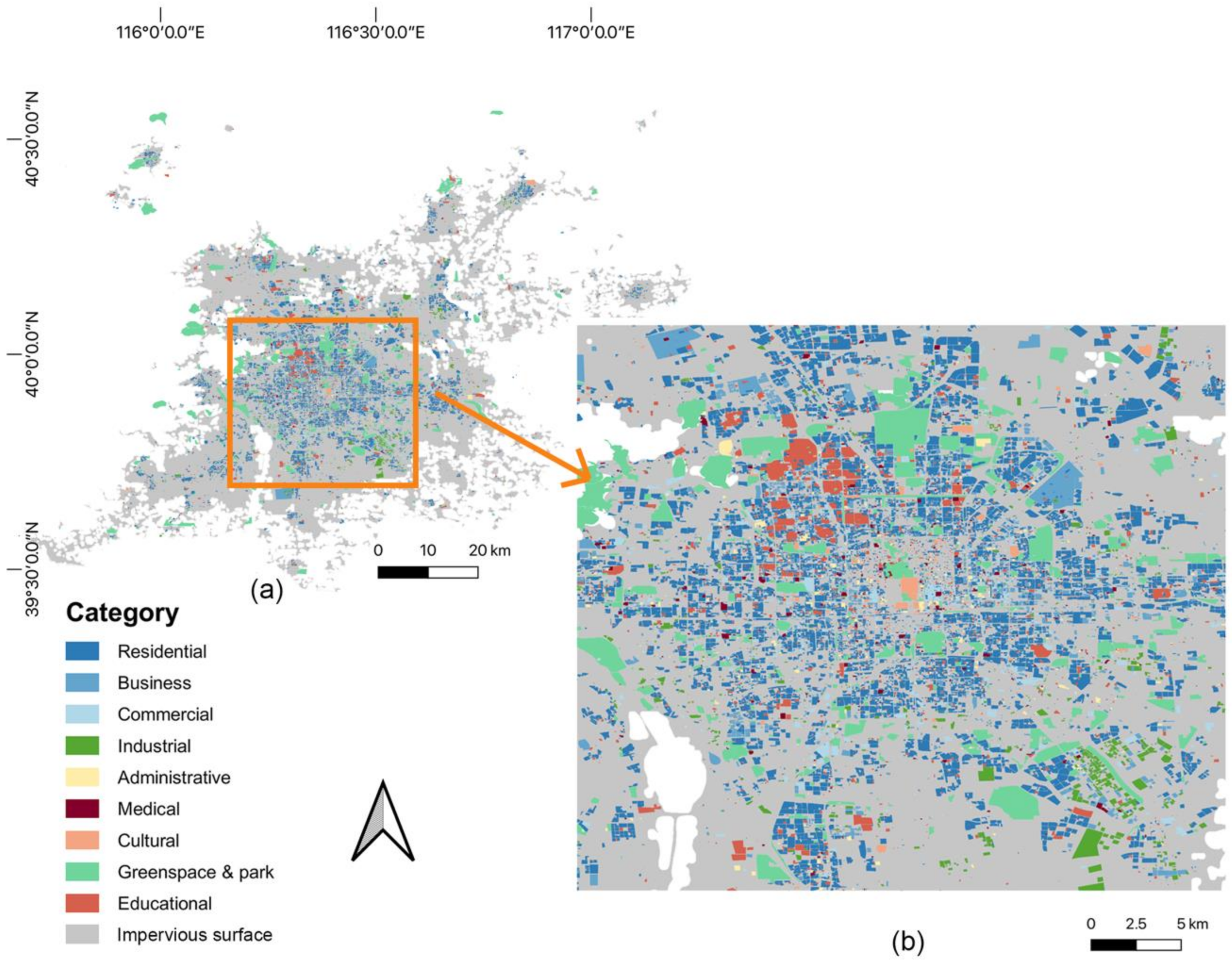
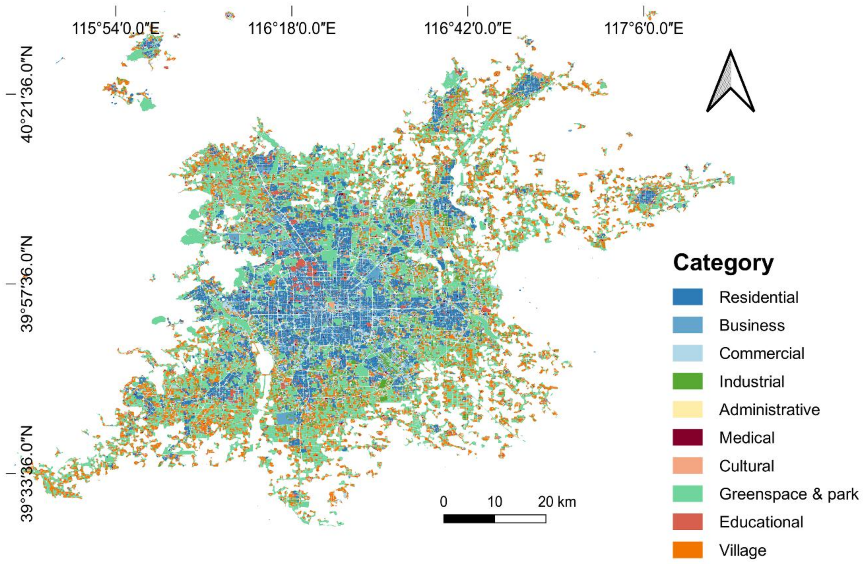
4.1. Mapping Results

Figure 8 shows most of the units were classified as a residential category with the original OSM units. Comparing Figure 8 with Figure 9, we can see that the proportion of the residential area was substantially reduced after a further decomposition of units. Many units at the urban fringe were classified as greenspace and village categories. Compared with the mapping results in Figure 9, the distribution pattern was increasingly detailed in Figure 10 and Figure 11, but the overall difference was small.

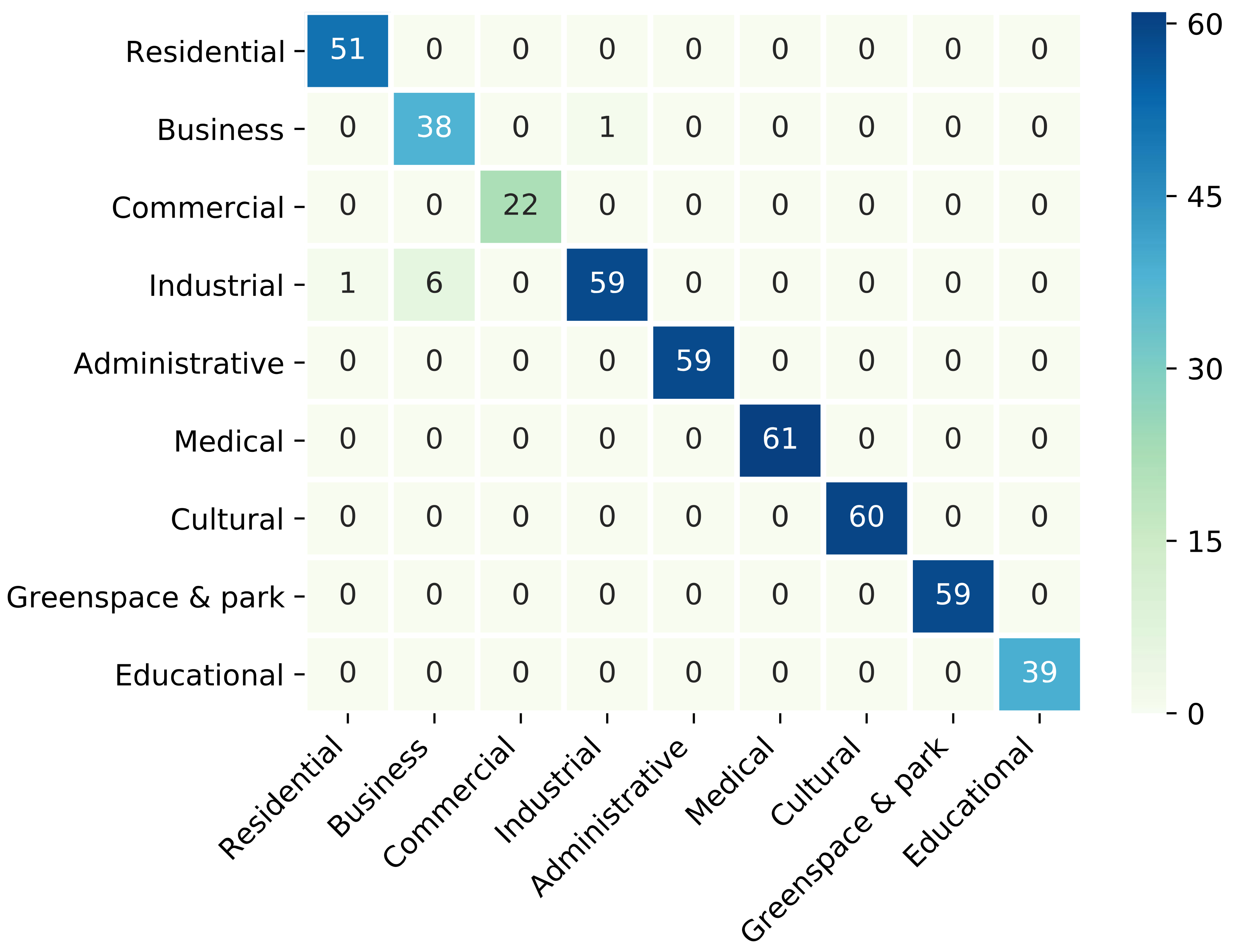
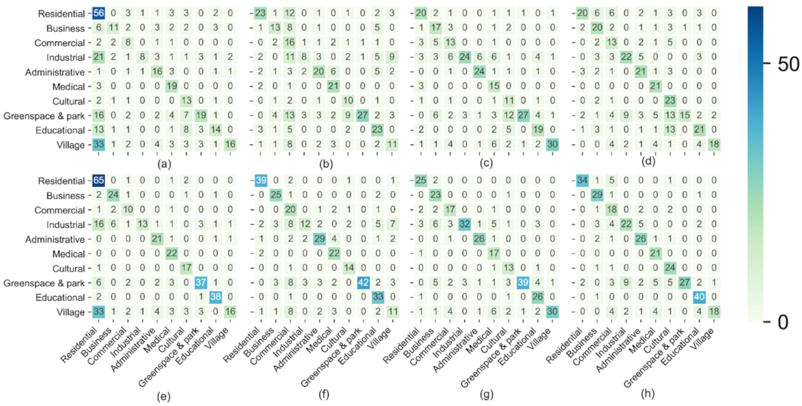
4.2. Accuracy Assessment of Mapping Results

Over 300 valid units were randomly selected and manually interpreted to conduct the accuracy assessment of the mapping results in each method. All validation units were surveyed through high resolution satellite image, Baidu Street View Service, and fieldwork.

Table 5. Accuracy assessment. OA, Kappa, and Support donate overall accuracy, Kappa coefficients, and the number of validation units, respectively.

Method	Before AOI Layer		After AOI Layer		Support
	OA	Kappa	OA	Kappa
OSM	48%	0.40	70%	0.66	377
OSM+300 m gird	50%	0.45	72%	0.68	345
OSM+200 m grid	62%	0.58	77%	0.74	323
OSM+100 m grid	57%	0.53	76%	0.74	340

shows the exact number of validation units used for each method, as well as the accuracy assessment results, including the overall accuracy (OA) and Kappa coefficients (Kappa). As the grid became smaller, both OA and Kappa increased. After integrating the AOIs layers, both OA and Kappa increased substantially. Using OSM and 200 m grid to generate classification units, we got the highest OA of 77% and Kappa of 0.74 after integrating the AOIs layers. Figure 12 presents the number of validation units in each category of the four methods. The least validation units used were in the commercial category of OSM methods with 14 sample units. The most validation units used were in the residential category of OSM methods with 69 units. Mostly, for a defined plan, the number of validation units in each category was no less than 20.

Comparing the two corresponding graphs above and below of Figure 13 we can see that integrating the AOIs layers resulted in a considerable rectification to classification results. From Figure 14, we found that after integrating the AOIs layers, UA and PA increased considerably.

4.3. Accuracy Assessment for Various Sample Size

Searching for the minimum sample size of stable classification accuracy, we used different numbers of AOIs as training samples. For each sample size, we repeated the experiment 20 times. The accuracy assessment was conducted using the same set of validation samples. We randomly selected AOIs of different numbers ranging from 5 percent to 95 percent in 5 percent intervals of all AOIs (24,346). Figure 15 illustrated the results. When the sample size reached 65 percent (15,824) of all AOIs, the classification results after integrating the AOIs layers reached stability.

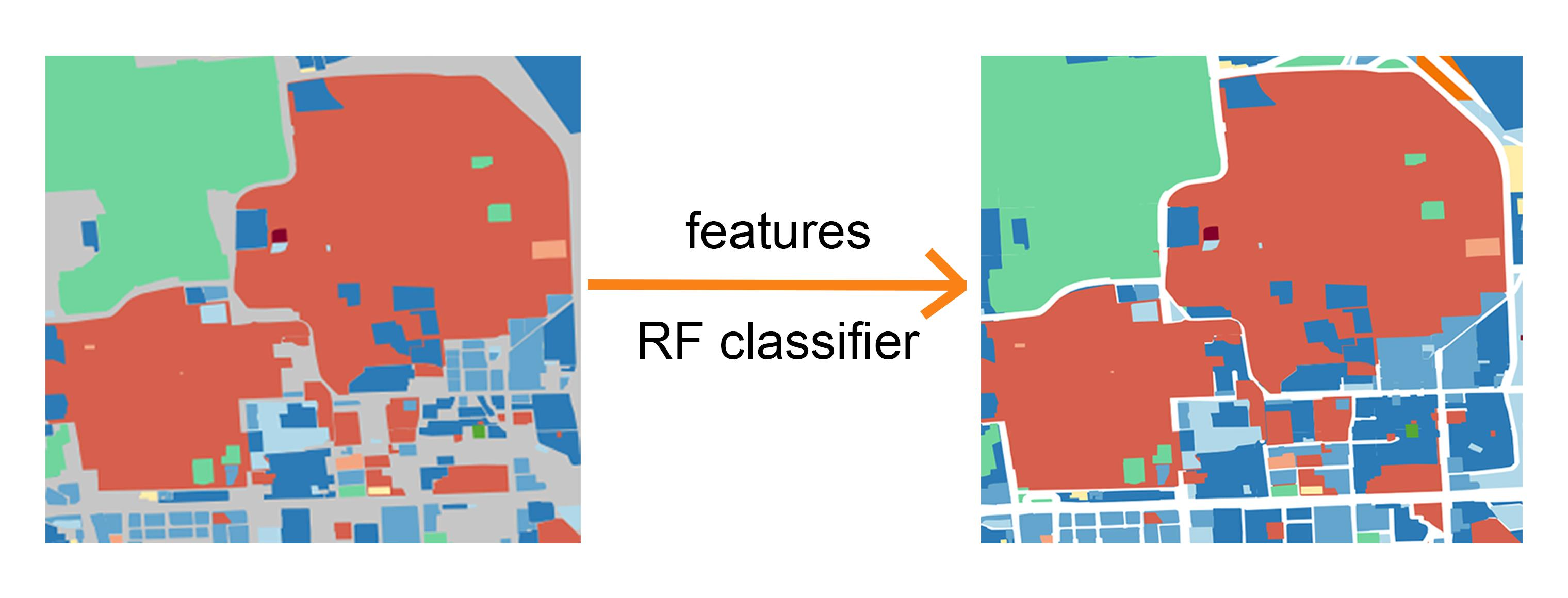
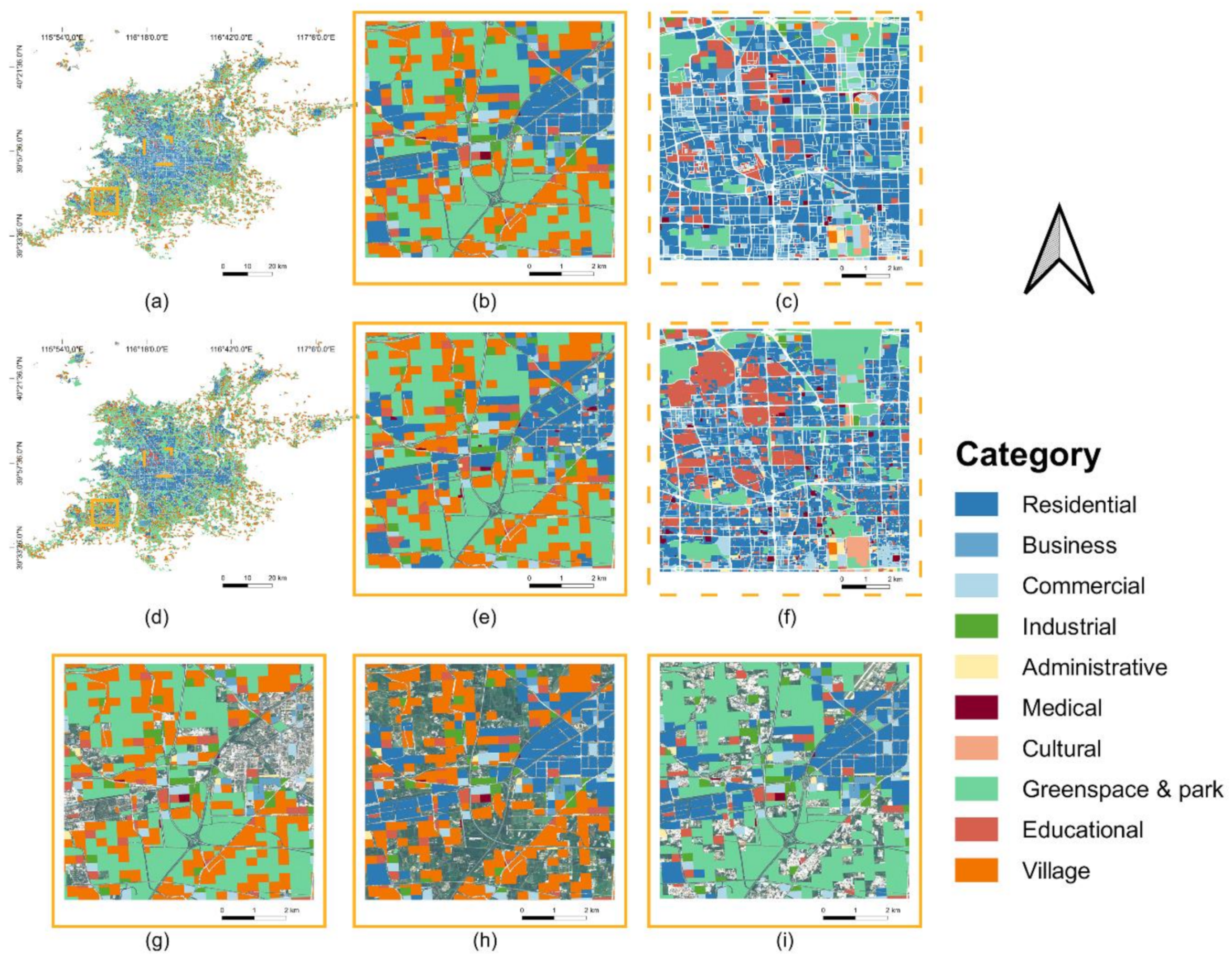
4.4. Comparison of Mapping Results before and after Integrating AOIs Layers

Comparing the differences between the update of Figure 16f to Figure 16c and the update of Figure 16e to Figure 16b, we found that the AOIs layers added much richer rectification and details to the urban centers than to the urban fringe area. It can be seen from Figure 16g–i, that a large number of units classified as residential at the urban fringe contained extensive area of greenspace and village categories. A comparison of Figure 17 with Figure 16 revealed similar results at the center, but Figure 17 provided more detailed information. For example, in Figure 16, the entire unit was marked as an administrative category, but in Figure 17, the whole unit was marked as a residential category, and the extent of the administrative category was marked more precisely with the help of AOIs layers. At the urban fringe, the classification in Figure 16 was more accurate and detailed. Figure 18 and Figure 19 offered more detailed information on the urban fringe area. Some administrative and medical units were scattered around the urban fringe. Administrative units mark the location of village committees and police stations, etc. Medical units mark the location of the village health center.

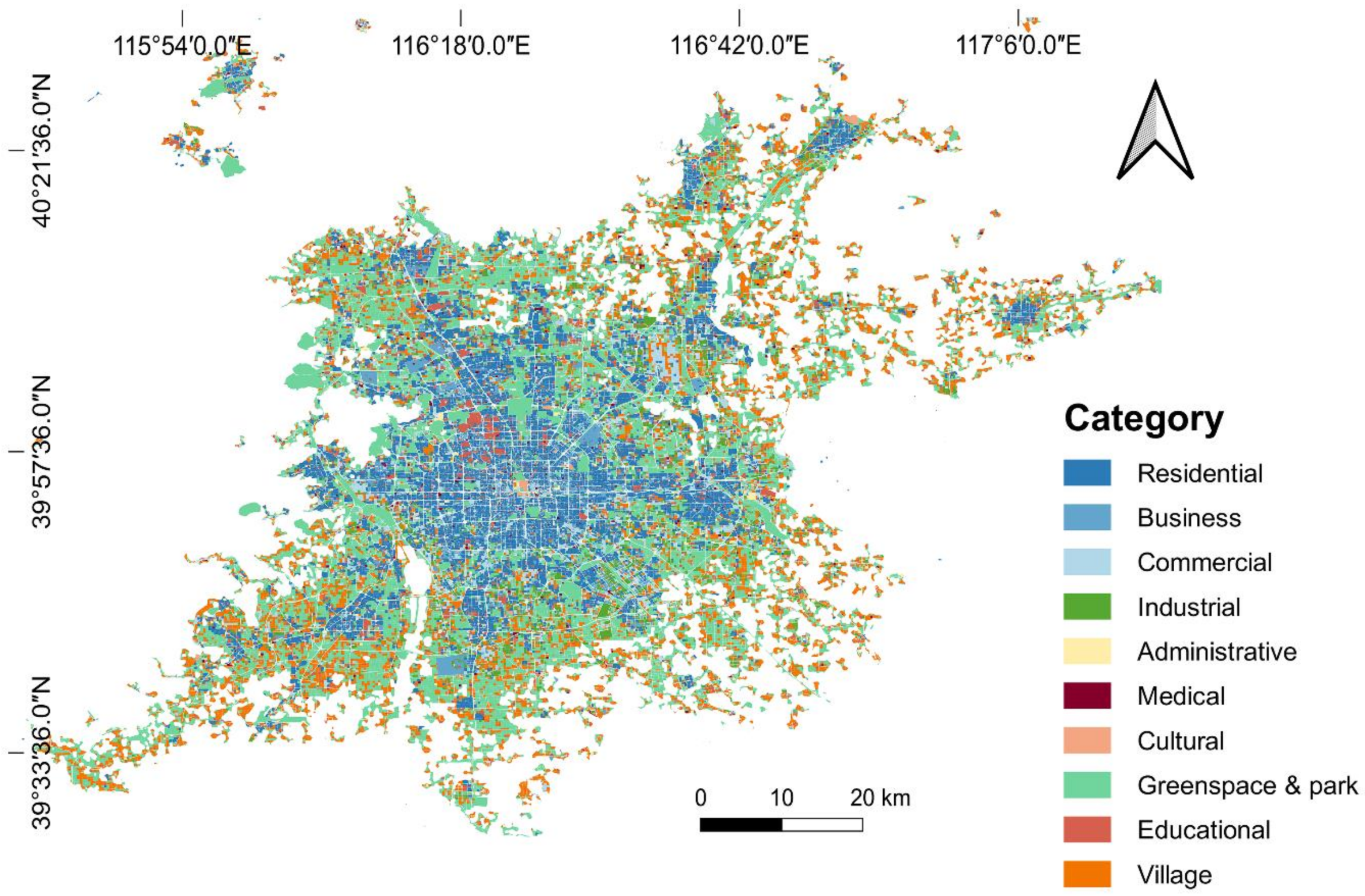
4.5. Comparison with EULUC Mapping Results

We compared the mapping results in this study with that in EULUC-China. Figure 20 and Figure 21 show the comparison for two locations at two scales, respectively. A large amount of administrative land is included in EULUC-China. In our results, the administrative extent is usually displayed with AOI data, only occupying the area as it is. Marking the whole unit as administrative category results in the loss of much valid information. When the same unit contains multiple educational, administrative, medical, and cultural categories, EULUC cannot handle it anymore, while our approach can still capture the results as they are.

5. Discussion

Using AOI data as the training sample significantly reduced labor-intensive sample collection work. The AOI data also provide a large number of the accurate extent of pure land uses. The mapping scheme proposed here is fast and stable to operate. After obtaining the nationwide AOI data with web crawlers, this scheme can be easily applied to cities across China.

In regions outside China, there is a lack of AOI data from the Baidu map used here. This makes it difficult to use AOI data as training samples. However, it is still possible to manually supplement the training sample by field survey or image interpretations. WorldPop data and OSM POI data can be used to replace Easygo Crowdedness data and Baidu map POI data, respectively. In this way, it is still feasible to classify urban land use with multi-source geospatial data and social data.

There are some limitations in our study that need to be improved in future works. First, we have a limited number of AOIs. The AOI data are mainly distributed in the urban centers but sparsely distributed in urban fringe areas. Image segmentation could be used [14] to extract building contours and assign them category information. In addition, the AOI data are prone to misclassification between business and industrial categories resulting in confusion between business and industrial categories in the mapping results. It is worth exploring how to classify the AOI data more accurately. In addition to the limitations of AOI data, the mixture of units needs to be addressed. Since most parcels are composed of mixed land uses, it is crucial to expand the classification from the current dominant-class only to multiple-class per parcel classification.

Choosing only Easygo Crowdedness data to represent people’s daily behavior is another limitation of this study. Further research is planned to include taxi GPS data, bus data, and subway data. In addition, there are some shortcomings in using geospatial big data to classify urban land use. For example, the activity frequency is closely related to the population density, which may be daily activities or noise caused by special events. Therefore, in future research, the classification of urban land use will be based on multisource data such as demographic data.

6. Conclusions

In this study, we overlaid the 300 m grid, 200 m grid, and 100 m grid to further divide the original OSM-based units of EULUC. Thus, units with more appropriate spatial sizes were obtained. AOI data were used as training samples, whose size was huge, and land use within the same unit was purer. This also eliminates data inconsistency in the crowdsourced collection due to subjective sample collection. After obtaining the classification results from the RF classifier, the AOIs layers were integrated with the classification results. Up to this step, we rectified some of the misclassification results and supplemented the land-use details to the building scale. As a result, we reached an overall accuracy of up to 77% with a Kappa coefficient of 0.74. We proposed a mapping scheme, which offers more detailed and accurate land-use information to the building scale, and significantly reduces labor-intensive sample collection work as compared to our previous EULUC mapping procedure. In addition, the scheme can be easily applied to cities across China.

References

1. Gong, P.; Liang, S.; Carlton, E.J.; Jiang, Q.; Wu, J.; Wang, L.; Remais, J.V. Urbanisation and health in China. Lancet 2012, 379, 843–852. [Google Scholar] [CrossRef]
2. Grimm, N.B.; Faeth, S.H.; Golubiewski, N.E.; Redman, C.L.; Wu, J.; Bai, X.; Briggs, J.M. Global Change and the Ecology of Cities. Science 2008, 319, 75–6760. [Google Scholar] [CrossRef] [PubMed] [Green Version]
3. Mao, W.; Lu, D.; Hou, L.; Liu, X.; Yue, W. Comparison of Machine-Learning Methods for Urban Land-Use Mapping in Hangzhou City, China. Remote Sens. 2020, 12, 2817. [Google Scholar] [CrossRef]
4. Lee, H.; Wang, J.; Leblon, B. Using Linear Regression, Random Forests, and Support Vector Machine with Unmanned Aerial Vehicle Multispectral Images to Predict Canopy Nitrogen Weight in Corn. Remote Sens. 2020, 12, 2071. [Google Scholar] [CrossRef]
5. Liu, Y.; Wang, L.; Zhang, B.; Men, J. Scene-level land use classification based on multi-features soft-probability cascading. Trans. Chin. Soc. Agric. Eng. 2016, 32, 266–272. [Google Scholar]
6. Yao, Y.; Liang, H.; Li, X.; Zhang, J.; He, J. Sensing Urban Land-Use Patterns by Integrating Google Tensorflow And Scene-Classification Models. arXiv 2017, arXiv:1708.01580. [Google Scholar] [CrossRef] [Green Version]
7. Fragou, S.; Kalogeropoulos, K.; Stathopoulos, N.; Louka, P.; Srivastava, P.K.; Karpouzas, S.P.; Kalivas, D.P.; Petropoulos, G. Quantifying Land Cover Changes in a Mediterranean Environment Using Landsat TM and Support Vector Machines. Forests 2020, 11, 750. [Google Scholar] [CrossRef]
8. Chakhar, A.; Ortega-Terol, D.; Hernández-López, D.; Ballesteros, R.; Ortega, J.F.; Moreno, M.A. Assessing the Accuracy of Multiple Classification Algorithms for Crop Classification Using Landsat-8 and Sentinel-2 Data. Remote Sens. 2020, 12, 1735. [Google Scholar] [CrossRef]
9. LaRocque, A.; Phiri, C.; Leblon, B.; Pirotti, F.; Connor, K.; Hanson, A. Wetland Mapping with Landsat 8 OLI, Sentinel-1, ALOS-1 PALSAR, and LiDAR Data in Southern New Brunswick, Canada. Remote Sens. 2020, 12, 2095. [Google Scholar] [CrossRef]
10. Morell-Monzó, S.; Estornell, J.; Sebastiá-Frasquet, M.-T. Comparison of Sentinel-2 and High-Resolution Imagery for Mapping Land Abandonment in Fragmented Areas. Remote Sens. 2020, 12, 2062. [Google Scholar]
11. Paoletti, M.; Haut, J.; Tao, X.; Plaza, J.; Plaza, A. A New GPU Implementation of Support Vector Machines for Fast Hyperspectral Image Classification. Remote Sens. 2020, 12, 1257. [Google Scholar] [CrossRef] [Green Version]
12. Hu, T.; Yang, J.; Li, X.; Gong, P. Mapping Urban Land Use by Using Landsat Images and Open Social Data. Remote Sens. 2016, 8, 151. [Google Scholar] [CrossRef]
13. Liu, X.; He, J.; Yao, Y.; Zhang, J.; Liang, H.; Wang, H.; Hong, Y. Classifying urban land use by integrating remote sensing and social media data. Int. J. Geogr. Inf. Sci. 2017, 31, 1675–1696. [Google Scholar] [CrossRef]
14. Tu, Y.; Chen, B.; Zhang, T.; Xu, B. Regional Mapping of Essential Urban Land Use Categories in China: A Segmentation-Based Approach. Remote Sens. 2020, 12, 1058. [Google Scholar] [CrossRef] [Green Version]
15. Gong, P.; Chen, B.; Li, X.; Liu, H.; Wang, J.; Bai, Y.; Chen, J.; Chen, X.; Fang, L.; Feng, S.; et al. Mapping essential urban land use categories in China (EULUC-China): Preliminary results for 2018. Sci. Bull. 2020, 65, 182–187. [Google Scholar] [CrossRef] [Green Version]
16. Su, M.; Guo, R.; Chen, B.; Hong, W.; Wang, J.; Feng, Y.; Xu, B. Sampling Strategy for Detailed Urban Land Use Classification: A Systematic Analysis in Shenzhen. Remote Sens. 2020, 12, 1497. [Google Scholar] [CrossRef]
17. Zong, L.; He, S.; Lian, J.; Bie, Q.; Wang, X.; Dong, J.; Xie, Y. Detailed Mapping of Urban Land Use Based on Multi-Source Data: A Case Study of Lanzhou. Remote Sens. 2020, 12, 1987. [Google Scholar] [CrossRef]
18. Sun, J.; Wang, H.; Song, Z.; Lu, J.; Meng, P.; Qin, S. Mapping Essential Urban Land Use Categories in Nanjing by Integrating Multi-Source Big Data. Remote Sens. 2020, 12, 2386. [Google Scholar] [CrossRef]
19. Hagenauer, J.; Helbich, M. Mining urban land use patterns from volunteered geographic information using genetic algorithms and artificial neural networks. Int. J. Geogr. Inf. Sci. 2012, 26, 963–982. [Google Scholar] [CrossRef]
20. Jokar Arsanjani, J.; Helbich, M.; Bakillah, M.; Hagenauer, J.; Zipf, A. Toward mapping land-use patterns from volunteered geographic information. Int. J. Geogr. Inf. Sci. 2013, 27, 2264–2278. [Google Scholar] [CrossRef]
21. Theobald, D.M. Development and applications of a comprehensive land use classification and map for the US. PLoS ONE 2014, 9, e94628. [Google Scholar] [CrossRef] [PubMed] [Green Version]
22. Vaz, E.; Jokar Arsanjani, J. Crowdsourced mapping of land use in urban dense environments: An assessment of Toronto. Can. Geogr./Géogr. Can. 2015, 59, 246–255. [Google Scholar] [CrossRef]
23. Forget, Y.; Linard, C.; Gilbert, M. Supervised Classification of Built-Up Areas in Sub-Saharan African Cities Using Landsat Imagery and OpenStreetMap. Remote Sens. 2018, 10, 1145. [Google Scholar] [CrossRef] [Green Version]
24. Grippa, T.; Georganos, S.; Zarougui, S.; Bognounou, P.; Diboulo, E.; Forget, Y.; Lennert, M.; Vanhuysse, S.; Mboga, N.; Wolff, E. Mapping Urban Land Use at Street Block Level Using OpenStreetMap, Remote Sensing Data, and Spatial Metrics. ISPRS Int. J. Geo-Inf. 2018, 7, 246. [Google Scholar] [CrossRef] [Green Version]
25. Gong, P.; Li, X.; Wang, J.; Bai, Y.; Chen, B.; Hu, T.; Liu, X.; Xu, B.; Yang, J.; Zhang, W.; et al. Annual maps of global artificial impervious area (GAIA) between 1985 and 2018. Remote Sens. Environ. 2020, 236, 111510. [Google Scholar] [CrossRef]
26. Louis, J.; Debaecker, V.; Pflug, B.; Main-Knorn, M.; Bieniarz, J.; Müller-Wilm, U.; Cadau, E.; Gascon, F. SENTINEL-2 SEN2COR: L2A Processor for Users. In Proceedings of the Living Planet Symposium, Prague, Czech Republic, 9–13 May 2016. [Google Scholar]
27. Li, X.; Zhao, L.; Li, D.; Xu, H. Mapping Urban Extent Using Luojia 1-01 Nighttime Light Imagery. Sensors 2018, 18, 3665. [Google Scholar] [CrossRef] [Green Version]
28. Li, F.; Zhang, F.; Li, X.; Wang, P.; Liang, J.; Mei, Y.; Cheng, W.; Qian, Y. Spatiotemporal Patterns of the Use of Urban Green Spaces and External Factors Contributing to Their Use in Central Beijing. Int. J. Environ. Res. Public Health 2017, 14, 237. [Google Scholar] [CrossRef]
29. Chen, B.; Song, Y.; Jiang, T.; Chen, Z.; Huang, B.; Xu, B. Real-Time Estimation of Population Exposure to PM2.5 Using Mobile- and Station-Based Big Data. Int. J. Environ. Res. Public Health 2018, 15, 573. [Google Scholar] [CrossRef] [Green Version]
30. Gong, P.; Marceau, D.J.; Howarth, P.J. A comparison of spatial feature extraction algorithms for land-use classification with SPOT HRV data. Remote Sens. Environ. 1992, 40, 137–151. [Google Scholar] [CrossRef]
31. Breiman, L. Random Forests. Mach. Learn. 2001, 45, 5–32. [Google Scholar] [CrossRef] [Green Version]
32. Gong, P.; Liu, H.; Zhang, M.; Li, C.; Wang, J.; Huang, H.; Clinton, N.; Ji, L.; Li, W.; Bai, Y.; et al. Stable classification with limited sample: Transferring a 30-m resolution sample set collected in 2015 to mapping 10-m resolution global land cover in 2017. Sci. Bull. 2019, 64, 370–373. [Google Scholar] [CrossRef] [Green Version]
33. Gong, P.; Wang, J.; Yu, L.; Zhao, Y.; Zhao, Y.; Liang, L.; Niu, Z.; Huang, X.; Fu, H.; Liu, S.; et al. Finer resolution observation and monitoring of global land cover: First mapping results with Landsat TM and ETM+ data. Int. J. Remote Sens. 2013, 34, 2607–2654. [Google Scholar] [CrossRef] [Green Version]
Figure 1. Map of the study area. The blue line shows the boundary of the administrative area of Beijing, China. The artificial impervious surface areas within Beijing are indicated by an orange boundary.
Remotesensing 13 00477 g001
Figure 2. Examples of manually interpreted land-use/land-cover categories from remote sensing imagery, indicated with orange boundaries. (a) Rural vegetation. (b) Urban greenspace. (c) Villages. (d) Residence.
Remotesensing 13 00477 g002
Figure 3. The workflow of the mapping scheme.
Remotesensing 13 00477 g003
Figure 4. The road network of central Beijing.
Remotesensing 13 00477 g004
Figure 5. Maps of AOI data. (a) The map of AOI data; (b) a zoomed-in view of (a).
Remotesensing 13 00477 g005
Figure 6. Confusion matrix for the accuracy assessment of AOI classification results.
Remotesensing 13 00477 g006
Figure 7. Histograms of features in remotely sensed data. The x-axis represents the value of features. The y-axis represents the probability density. The total number of bins for each graph is 100. Data less than the 1st quartile and greater than the 99th quartile are not shown. (a) Histograms of Mean of B, G, R, and NIR bands. (b) Histograms of the standard deviation of B, G, R, and NIR bands. (c) Histograms of features of NDVI and NDWI index. (d) Histograms of features of luojia nighttime light imagery.
Remotesensing 13 00477 g007
Figure 8. Map of EULUC-AOI (OSM) in Beijing, 2019.
Remotesensing 13 00477 g008
Figure 9. Map of EULUC-AOI (OSM+300 m grid) in Beijing, 2019.
Remotesensing 13 00477 g009
Figure 10. Map of EULUC-AOI (OSM+200 m grid) in Beijing, 2019.
Remotesensing 13 00477 g010
Figure 11. Map of EULUC-AOI (OSM+100 m grid) in Beijing, 2019.
Remotesensing 13 00477 g011
Figure 12. The number of validation units in each category of the four methods. Support donates the number of validation units.
Remotesensing 13 00477 g012
Figure 13. Confusion matrix for accuracy assessment of mapping results of EULUC-AOI in Beijing, 2019. (ad) The confusion matrix before integrating the AOI layers of OSM, OSM and 300 m grid, OSM and 200 m grid, and 100 m grid in turn; (eh) The confusion matrix after integrating AOIs layers of OSM, OSM and 300 m grid, OSM and 200 m grid, and OSM and 100 m grid in turn.
Remotesensing 13 00477 g013
Figure 14. Accuracy assessment of mapping results of EULUC-AOI in Beijing, 2019. UA and PA donate user’s accuracy and the producer’s accuracy, respectively.
Remotesensing 13 00477 g014
Figure 15. Overall accuracy assessment of classification results after integrating AOIs layers. The two black whiskers extend from the first quartile to the smallest value and from the third quartile to the largest value. The median is shown with an orange line. Extreme values are indicated with symbol of ☆. The horizontal red dashed line shows the value at which the overall accuracy has stabilized, and the vertical red dashed line represents the first experiment in which the overall accuracy is stable.
Remotesensing 13 00477 g015
Figure 16. Comparison and zoomed-in views of EULUC-AOI (OSM) in Beijing, 2019. (a) The mapping results before overlaying the AOIs layers; (b,c) zoomed-in views of (a); (d) the mapping results after overlaying the AOIs layers; (e,f) zoomed-in views of (d); the zoomed-in views with solid lines outside shows details in the solid box in the lower-left corner of the mapping results. The zoomed-in view with dashed lines outside shows details in the dashed box near the middle of the mapping results. (gi) The results of (b) with the removal of residential, greenspace, and village units in turn, with Sentinel II optical images in the background.
Remotesensing 13 00477 g016
Figure 17. Comparison and zoomed-in views of EULUC-AOI (OSM+300 m grid) in Beijing, 2019. (a) The mapping results before overlaying the AOIs layers; (b,c) zoomed-in views of (a); (d) the mapping results after overlaying the AOIs layers; (e,f) zoomed-in views of (d); the zoomed-in views with solid lines outside shows details in the solid box in the lower-left corner of the mapping results. The zoomed-in view with dashed lines outside shows details in the dashed box near the middle of the mapping results. (gi) The results of (b) with the removal of residential, greenspace, and village units in turn, with Sentinel II optical images in the background.
Remotesensing 13 00477 g017
Figure 18. Comparison and zoomed-in views of EULUC-AOI (OSM+200 m grid) in Beijing, 2019. (a) The mapping results before overlaying the AOIs layers; (b,c) zoomed-in views of (a); (d) the mapping results after overlaying the AOIs layers; (e,f) zoomed-in views of (d). The zoomed-in views with solid lines outside show details in the solid box in the lower-left corner of the mapping results. The zoomed-in view with dashed lines outside shows details in the dashed box near the middle of the mapping results. (gi) The results of (b) with the removal of residential, greenspace, and village units in turn, with Sentinel II optical images in the background.
Remotesensing 13 00477 g018
Figure 19. Comparison and zoomed-in views of EULUC-AOI (OSM+100 m grid) in Beijing, 2019s. (a) The mapping results before overlaying the AOIs layers; (b,c) zoomed-in views of (a); (d) the mapping results after overlaying the AOIs layers; (e,f) zoomed-in views of (d); the zoomed-in views with solid lines outside shows details in the solid box in the lower-left corner of the mapping results. The zoomed-in view with dashed lines outside shows details in the dashed box near the middle of the mapping results. (gi) The results of (b) with the removal of residential, greenspace, and village units in turn, with Sentinel II optical images in the background.
Remotesensing 13 00477 g019
Figure 20. Comparison of the mapping results in this study with that in EULUC-China. (a,c) Zoomed-in views of the mapping results of EULUC; (b,d) zoomed-in views of the mapping results in this study.
Remotesensing 13 00477 g020
Figure 21. Comparison of the mapping results in this study with that in EULUC-China. (a,c) Zoomed-in views of the mapping results of EULUC; (b,d) zoomed-in views of the mapping results in this study.
Remotesensing 13 00477 g021