Abstract
Water scarcity is one of the most important problems of agroecosystems in Mediterranean and semiarid areas, especially for species such as vineyards that largely depend on irrigation. Actual evapotranspiration (ET) is a variable that represents water consumption of a crop, integrating climate and biophysical variables. Actual evapotranspiration models based on remote sensing data from visible bands of Sentinel-2, including Penman-Monteith–Stewart (RS-PMS) and Penman-Monteith–Leuning (RS-PML), were evaluated at different temporal scales in a Cabernet Sauvignon vineyard (Vitis vinifera L.) located in central Chile, and their performance compared with independent ET measurements from an eddy covariance system (EC) and outputs from models based on thermal infrared data from Landsat 7 and Landsat 8, such as Mapping EvapoTranspiration with high Resolution and Internalized Calibration (METRIC) and Priestley–Taylor Two-Source Model (TSEB-PT). The RS-PMS model showed the best goodness of fit for all temporal scales evaluated, especially at instantaneous and daily ET, with root mean squared error (RMSE) of 28.9 Wm−2 and 0.52 mm day−1, respectively, and Willmott agreement index (d1) values of 0.77 at instantaneous scale and 0.7 at daily scale. Additionally, both approaches of RS-PM model were evaluated incorporating a soil evaporation estimation method, one considering the soil water content (fSWC) and the other hand, using the ratio of accumulated precipitation and equivalent evaporation (fZhang), achieving the best fit at instantaneous scale for RS-PMS fSWC method with relative root mean squared error (%RMSE) of 15.2% in comparison to 58.8% of fZhang. Finally, the relevance of the RS-PMS model was highlighted in the assessment and monitoring of vineyard drip irrigation in terms of crop coefficient (Kc) estimation, which is one of the methods commonly used in irrigation planning, yielding a comparable Kc to the one obtained by the EC tower with a bias around 9%.
1. Introduction
Water is becoming increasingly scarce, especially for agricultural activities, and its demand for agricultural purposes is projected to increase 60% by 2050 [1], especially in irrigated crops [1,2,3,4,5]. Vineyards (Vitis vinifera L.) located in arid, semi-arid and Mediterranean climates are especially sensitive to changes in water availability which affects not only yield but also the quality of wines [6,7,8,9,10]. A key element for water management in vineyards is the accurate measurement of water use via evapotranspiration (ET) both in time and space. Obtaining this type of information is now possible through remote sensing-based data [11,12,13,14,15,16] and models that use retrieved information to assess evapotranspiration.
Remote sensing-based ET models are classified in two different groups depending on the type of information used: (a) models based on thermal infrared bands (TIR-ET), and (b) models based on visible and near-infrared bands (VIS-ET) [17].
TIR-ET models are capable of estimating land surface temperature (LST) from thermal infrared remote sensing data, allowing the determination of plant water status [11]. Examples of TIR-ET models are the Mapping Evapotranspiration at High Resolution with Internalized Calibration (METRIC) [18], that includes a correction to mitigate atmospheric effects on surface temperature, and uses an internal calibration to reduce bias in aerodynamic stability or surface roughness, based on the selection of a hot (dry surface) and cold (wet surface) pixel. In addition, METRIC estimates ET by considering the value of evapotranspiration from a well irrigated reference crop (ET0). However large differences in the results have been reported due to the selection of hot/cold pixels within the evaluated scene [19].
In vineyards, the use of TIR-ET models has been assessed. Examples are the Surface Energy Balance Algorithm for Land (SEBAL) [20], METRIC [21,22,23], the Simplified Surface Energy Balance Index (S-SEBI) [24,25], the Simplified Two-Source Energy Balance (STSEB) [26], the Atmosphere–Land Exchange Inverse (ALEXI) model and its flux disaggregation scheme (DisAlexi) [27,28] and the two-source energy balance (TSEB) model [20,23,29,30,31].
However, accuracy of TIR-ET models depends on temporal and spatial scale of thermal infrared (TIR) bands. As their spatial resolution ranges between 30–120 m, Landsat 5, Landsat 7 and Landsat 8 satellites have been widely used at field scale. Nevertheless, the 16-day frequency of temporal resolution of these products, limit their use for irrigation management purposes [11,32,33].
VIS-ET models have the advantage of using vegetation indices (VIs) to estimate ET, which are simple to obtain and are strongly correlated with the biophysical characteristics of canopy associated with ET, such as leaf area index (LAI), a fraction of absorbed PAR radiation (fAPAR) and vegetation cover (fC) [11,13]. As TIR-ET models, VIS-ET are limited by usual tradeoff between spatial and temporal scale of remote sensing data.
The launch of Sentinel-2 satellite in 2015, which captures data within visible and near infra-red spectrum, at a spatial resolution between 10–20 m and temporal resolution of 3–5 days, opens an opportunity to circumvent those problems and becomes an appropriate data source for ET monitoring and irrigation assessment. Only recently there has been methods that are based on this type of the information, with some reports of successful use in crops such as tomato [34], cotton [35], irrigated barley and wheat (in combination with Landsat 8 data) [36], irrigated corn-soybean, vineyard and potato, the latter through a data fusion method between Sentinel-2 and Sentinel-3 satellites [23,37].
The performance of the VIS-ET (FAO-56) and TIR-ET (TSEB) models has been compared in an orange orchard in Mediterranean climate and under drip irrigation conditions, highlighting that although the FAO-56 model has the advantage that it delivers daily ET without scaling from instantaneous values, the TIR-ET models yielded the best fit when compared with EC measurements. Similarly, ET is modeled via FAO-56 method for table grapes in absence of water stress using Landsat 8 and RapidEyes data, obtaining good agreement with independent eddy-covariance measurements [38]. Nevertheless, it is highlighted that the estimations obtained from the proposed method depend on ET0, precipitation, phenology and canopy cover at each site, thus Kcb values are site specific.
The Penman-Monteith equation has been coupled with remote sensing data for evapotranspiration modeling (RS-PM), based on the combination of energy balance and a mass transfer method that incorporates resistance or conductance factors. Two RS-PM models were evaluated using Landsat 5 and Landsat 7 data, establishing the strong dependency between ET and soil water content, especially in irrigated vineyards and orchards, since a larger fraction of net radiation (RN) is allocated to instantaneous latent heat flux (λE) and not to instantaneous sensible heat flux (H), as would occur on dryland vineyards [39].
Several approaches have been proposed to improve RS-PM model, focusing on the estimation of surface conductance. In this regard, the vegetation conductance has been modeled from the LAI estimated with remote sensing data, using initially Moderate Resolution Imaging Spectroradiometer (MODIS) data that have a pixel resolution of 1000 m [40]. Despite the good agreement on magnitudes and seasonal variation in both ecosystems, the method is limited to areas where the LAI is greater than 2, since it is assumed that the canopy cover a large proportion of the soil and thus the surface conductance (gs) is approximate to the canopy conductance (gc).
Likewise, Leuning and collaborators [41] introduced improvements to the previous models regarding the modeling of gc and soil evaporation (RS-PML). Thus, gc is modeled as a function of maximum leaf stomatal conductance at the top of the canopy (gsx), LAI, Da and the hyperbolic response to absorbed short-wave radiation [42], which is easily parameterized and coupled with a photosynthesis function, but does not respond to water stress, an important factor in irrigated vineyards under Mediterranean climates. Additionally, soil evaporation is assumed as a constant fraction (f) of the equilibrium evaporation rate of soil surface, although that should be adjusted according to soil water content. However, RS-PML had good agreement when assessed in 15 sites at a spatial resolution of 1000 m, including vegetation cover of savannah, annual crops, and diverse forest classes. Authors modeled daily f as a function of soil water content [43,44], which improved the estimation of soil evaporation and thus the estimation of total ET, especially in dryland sparse vegetation.
Based on the aforementioned, modeling ET based on the Penman-Monteith equation and Sentinel-2 data in drip irrigated vineyards, the RS-PM approach should be improved incorporating soil water content data as one of the environmental variables that controls both stomatal conductance and the soil evaporation fraction. Thus, the model of stomal conductance proposed by Stewart [45] is an empirical approach based on a multiplicative environmental function from solar radiation, air temperature, vapor pressure deficit and soil water deficit, which is suitable to be coupled with the RS-PM model, hereinafter referred as Remote Sensing Penman-Monteith–Stewart model (RS-PMS). Therefore, it is hypothesized that RS-Penman-Monteith model integrated with Sentinel-2 data and coupled to a function that adjusts the stomatal conductance and soil evaporative fraction according to soil water content (RS-PMS), improves the goodness of fit of modeled actual ET. Hence, the general objective of this research was to evaluate the Penman-Monteith model for remote sensing data, based on the Leuning approach (RS-PML) and a novel approach that incorporates the Stewart stomatal conductance model (RS-PMS), on a drip irrigated vineyard located in central Chile by comparing independent data from an eddy covariance system and the METRIC and TSEB-PT models.
2. Materials and Methods
2.1. Study Area
The study was carried on in a drip irrigated vineyard (Vitis vinifera L. cv. Cabernet Sauvignon) during the 2017–2018 (S1) and 2018–2019 (S2) growing seasons. The Vineyard is in central Chile, 40 km south of the city of Santiago. The area is characterized by Mediterranean climate with annual average temperatures of 18 °C; precipitations are concentrated in winter (June-September) with an average annual total of 280 mm. The soil is characterized by Mollisol order with predominantly loamy texture within the first 0.6 m and sandy loam between 0.6 and 1 m of depth; bulk density varies between 1.38 and 1.48 g cm−3 within one meter of depth.
The vineyard was planted in 2010, rows oriented north-south with 2.5 m between rows and 1.0 m between vines. The aisles are maintained vegetation-free using mechanical and chemical weed controls; fertilization management is used to avoid nutritional deficiencies of both macro and micro elements. The amount of water applied by drip irrigation during the season was calculated as a function of reference crop evapotranspiration (ET0), applying 50% of ET0 (ET0 × 0.5) with frequencies of 7 days throughout the season and an irrigation time that varied between 8 and 10 h. The applied irrigation corresponds to the gross water demand and the total amount irrigated was measured with a flow meter, applying 481 mm in S1 and 334 in S2. Additionally, the irrigation system has a single irrigation line, with two emitters per plant spaced at 0.4 m and a flow rate of 4.1 L s−1 per emitter. In each irrigation event, wetted area uniformity was observed with some cases where superficial water runoff was evidenced, which corresponded to less than 5% of the emitters. Canopy management was different in the two growing seasons. In S1 the trellis system was vertical-shoot-positioned with three wire lines, while in S2 the training system was without wire lines, increasing the frequency of pruning during the growing season.
2.2. Field Measurements
Ground and remote sensing data are the input of both VIS-ET and TIR-ET models (Figure 1), which are described in the following sections. Field measurements included micrometeorological, phenological and fraction of radiation transmitted by canopy. The micrometeorological data were obtained through an eddy covariance system (EC) measuring exchanges of energy and mass between the vineyard and the atmosphere [46]. Due to the prevailing wind direction during daylight hours, a west-facing EC tower was installed in the east border of the study area (Figure 2), with coordinates 33°42’16”S and 70°34’32”.
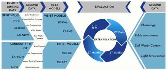
Figure 1.
Data sources and their integration with Remote Sensing-based Evapotranspiration (ET) models (RS-ET models). NDVI = Normalized Differential Vegetation Index; LAI-NDVI = Leaf Area Index obtained by NDVI; LST = Land Surface Temperature; RS-PML: Remote Sensing Penman-Monteith–Leuning Model; RS-PMS = Remote Sensing Penman-Monteith–Stewart Model; METRIC = Mapping EvapoTranspiration with high Resolution and Internalized Calibration; TSEB-PT = Priestley–Taylor Two-Source Model; λE = Instantaneous Evapotranspiration; ET-Daily = Cumulative Daily Evapotranspiration; ET-Weekly = Cumulative Weekly Evapotranspiration; ET-Monthly = Cumulative Monthly Evapotranspiration.
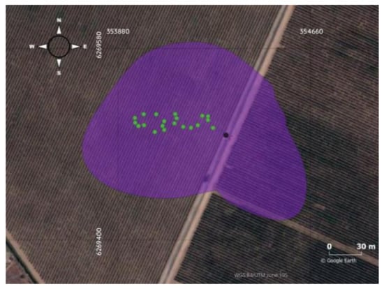
Figure 2.
Vineyard study area and climatological footprint. Black dot is eddy covariance system (EC) localization. Purple line contour is footprint 90% flux source area. Green dots are places where phenology and radiation intercepted by canopy were measured.
The EC was equipped with an open-path infrared gas analyzer integrated with a 3D sonic anemometer model IRGASON (Campbell Scientific Inc., Logan, UT, USA), placed 4 m above the ground surface and sampling frequency of 10 Hz. Other measuring devices in place were temperature and relative humidity HMP45C sensors (Campbell Scientific Inc., Logan, UT, USA); photosynthetically active radiation (PAR) model LI190SB (Campbell Scientific Inc. Logan, UT, USA) device; net radiometer model NR Lite2 (Kipp and Zonen B.V., The Netherlands), placed 0.5 m above the top of the vineyard canopy, which is representative of both the bare soil surface and the vegetative surface covered by the vine; two soil heat plates model HFP01-L (Campbell Scientific Inc., Logan, UT, USA), with 0.9 m of separation and 0.08 m below the soil surface. Additionally, there were two thermocouples model TCAV (Campbell Scientific Inc., Logan, UT, USA) at 0.05 m of depth and one Time Domain Reflectometry model CS616 (Campbell Scientific Inc., Logan, UT, USA) at 10 cm of depth. The data from these sensors were processed by a CR3000 datalogger (Campbell Scientific Inc., Logan, UT, USA).
Traditional EC raw data quality controls were performed [47,48], including spike removal, double coordinate rotation [49], correction for frequency loss [50], air density [51] and turbulent and stationarity conditions [52]. Additionally, an analysis of energy balance closure was made, which means a linear regression between the sum of latent and sensitive heat flux (λE + H) and the subtraction between net radiation and soil heat flux (RN − G) or available energy (A) [53]. The EC data analysis was synthesized in 30-min averages and the climatological flux footprint was parameterized based on the crosswind distribution [54] in order to overlap with remote sensing data and evaluate model outputs, considering the footprint contour encompass 90% of the total flux [55,56,57].
In addition, EC measurements were complemented with meteorological data collected from the William Fevre agrometeorological station (33°67’S and 70°58’W), located 4 km north of the study area. This station records solar radiation (MJ m−2 day−1), air temperature (°C), relative humidity (%), wind speed (m s−1) and precipitation (mm).
The EC footprint was divided according to Landsat 8 pixels (green dots in Figure 2) and vines located within the pixels were randomly selected, in order to observe phenology and measure fraction of radiation transmitted by canopy (fTPAR). Phenological observations were made every 7 days during S1 and S2 according to BBCH-scale [58], which assigns a decimal code to each phenological stage ranging from 00 to 99 and in vineyards were identified the beginning of Leaf development (BBCH-11), Inflorescence emergence (BBCH-53), Flowering (BBCH-61), Development of fruits (BBCH-71) and Ripening of berries (BBCH-81). The criterion used to identify a phenological stage was when 50% of the vines had reached the next phenological stage (Table 1).

Table 1.
Description of vineyard phenology according to BBCH scale [58].
Finally, fTPAR was measured at 20 points within the EC footprint as was made with phenological observation. Those points are obtained from samples made across the row in three consecutive vines each spaced by 0.3 m with a LAIPen LP 100 sensor (Photon Systems Instruments, Czech Republic), which has been used in forest canopy characterization [59,60,61]. The LAIPen LP 100 measures the gap fraction of blue band of the photosynthetically active radiation (0.4–0.5 µm), which is the most efficiently absorbed spectral band by leaf pigments and similar to LAI-2000 (LI-COR, Lincoln, NE, USA), removes radiation with wavelengths higher than 0.5 µm at which scattering is more pronounced. All measurements were made before 11:00 am in order to reduce the influence of high zenith angles.
Moreover, assuming that vineyard canopy is a homogeneous turbid medium, where leaves are randomly distributed within the canopy, and individual leaf size is small when is compared with the canopy, one LAIPen LP 100 equipment measured below the canopy (Rbelow) and simultaneously a second equipment measured on top of the canopy (Rtop). With these measurements, fTPAR is calculated as the ratio Rbelow/Rtop and applying a light extinction model [62] is estimated the Leaf Area Index (LAIE) as an indirect measurement of LAI:
where k is canopy extinction coefficient, set in a value of 0.5 in previous measurements on a Cabernet Sauvignon vineyard [63]. Then, LAIE was adjusted (LAIEA) assuming that vineyard canopy is composed of 82% of wood (trunk, cordons and canes) by volume of surface area [64], and by inter-row space factor of 0.40, which was obtained from the ratio of vines space (1.0 m) and inter-row space (2.5 m) [65]:
2.3. Remote Sensing Data
Remote sensing data was obtained from Landsat 7, Landsat 8 and Sentinel-2 missions, with each mission having different temporal, spatial, spectral and radiometric resolution (Table 2). Landsat 7 and Landsat 8 (Landsat 7–8) have a 16-day repeat cycle, both within visible (σblue, σgreen, σred) and near-infrared (σnir) bands have pixel resolution of 30 m, while within thermal infrared band (σtir) Landsat 7 has a pixel resolution of 60 m and Landasat 8 of 100 m, with a resampling to 30 m [66]. Sentinel-2 visible and near-infrared bands have a spatial resolution of 10 m with temporal frequency of 5 days at latitudes near to equator and 2–3 days at mid latitudes [67]. The remote sensing data were filtered by date during the growing season and by percentage of cloudiness lower than 10% for Landsat 7–8 and lower than 30% for Sentinel-2. In Landsat 7-8 a lower percentage of cloudiness was used, since this data source uses the TIR band for Land Surface Temperature (LST) estimation, which generates a large amount of noise when the percentage of cloudiness is higher than 10%.
Table 2.
Spatial resolution of remote sensing data.
The Normalized Difference Vegetation Index (NDVI) was calculated from Landsat 7–8 and Sentinel-2 data (Table 3), in order to model the Leaf Area Index (LAINDVI). Previously the noise associated with NDVI was removed through Savitzky–Golay’s algorithm [68] and therefore, a regression analysis was performed between NDVI and LAIEA to model LAINDVI for each set of remote sensing data. In addition, the fraction of vegetation cover (fC) was calculated as a function of LAINDVI and the viewing angle of the sensor (θ) [69]:
Table 3.
Parameters and number of images from remote sensing data.
The LST was calculated from thermal bands of Landsat 7 (10.4–12.5 µm) and Landsat 8 (10.6–11.2 µm) according to the Single Channel Algorithm method (SC) [70,71], which is appropriate when one single thermal band of the sensor is available. Furthermore, SC method is based on surface emissivity (εS) and radiance (Lsen), brightness temperature (Tsen), transmissivity (τ) and downward (Ld) and upward (Lu) radiance as atmospheric variables. The atmospheric variables were obtained from the National Center for Environmental Prediction (NCEP), that is a global tropospheric analyses product providing atmospheric profiles every 6h at resolution of 1° × 1° [72], and it is available in the data catalog of Google Earth Engine (https://developers.google.com/earth-engine/datasets/catalog/NCEP_RE_surface_temp#description).
The calculation of NDVI (https://code.earthengine.google.com/2f17d6fd8809f2ca1a21448c1c61b653) and LST (https://code.earthengine.google.com/4c0f3d0af6df02bf6a88ba96e046f711) was supported by Google Earth Engine (GEE), a cloud-based platform for spatial data analysis [73]. GEE is based on JavaScript code for geospatial analysis and in addition provides access to several remote sensing data bases including Landsat 7, Landsat-8, Sentinel-2 and NCEP, which allow the data assimilation process with minimum computational capabilities.
The overlapping of remote sensing grid and EC climatological flux footprint were grouped in 22 pixels for Landsat 7–8 and 108 pixels for Sentinel-2, which are averaged in order to compare with 90% source area of EC climatological flux footprint [74].
2.4. Remote Sensing-Based ET Models
The Remote Sensing Penman-Monteith–Stewart model (RS-PMS) is evaluated and compared with the Remote Sensing Penman-Monteith–Leuning (RS-PML), the Mapping Evapotranspiration at High Resolution with Internalized Calibration (METRIC) and the Priestley–Taylor Two Source Energy Balance (TSEB-PT). Table 4 summarizes the main features of evaluated models.
Table 4.
Main features of the models Mapping Evapotranspiration at High Resolution with Internalized Calibration (METRIC), Priestley–Taylor Two Source Energy Balance (TSEB-PT), Remote Sensing Penman-Monteith–Leuning (RS-PML) and Remote Sensing Penman-Monteith–Stewart (RS-PMS).
2.4.1. Mapping Evapotranspiration at High Resolution with Internalized Calibration (METRIC)
The instantaneous λE (Wm−2) is calculated in METRIC [18] as a residual of the energy balance equation:
where RN is net radiation (Wm−2); α the surface albedo; εs the surface emissivity; RS the solar radiation (Wm−2); RLd the downward longwave radiation (Wm−2) determined empirically by air transmissivity; RLu is upward longwave radiation (Wm−2) obtained by thermal band. Therefore, shortwave and longwave net radiation are calculated following the approach suggested by [75].
The soil heat flux (G) is calculated as a fraction of RN based on field measurements, and H (W m−2) is calculated following the equations:
where ρa is air density (kg m−3); Cp air specific heat at constant pressure (J kg−1 K−1); ΔT vertical temperature difference near the surface (K); rah (s m−1) aerodynamic resistance corresponding to ΔT; and c and m are parameters empirically determined in the image. ΔT and rah are derived from the information of two selected pixels in the evaluated scene or image, called the "cold pixel" and "hot pixel", which refer to a wet and dry surface, respectively. The λE for each of these pixels is assigned by operators, in order to derive H using Equation (4). Thus, the combined values of ΔT and rah are iteratively obtained assuming an initial condition of neutral stability and subsequently is corrected by atmospheric stability conditions, which depends on the length of Monin–Obukhov for both the wind speed at satellite overpass and the surface roughness length [18,76,77].
2.4.2. Priestley–Taylor Two Source Energy Balance (TSEB-PT)
As in METRIC, which estimates λE as residual of surface energy balance (Equation (4)), TSEB-PT estimates resistances of both canopy and soil surfaces, splitting the energy balance components between canopy and soil [78]:
where instantaneous fluxes are expressed in Wm−2, and subscripts refer to canopy (C) and soil (S). Here G is a fraction of RN obtained from EC measurements.
Therefore, total (H), canopy (HC) and soil (HS) heat fluxes are given by:
where TA is air temperature (K); TAC is the temperature in the air-canopy space (K); TS is soil surface temperature; rA aerodynamic resistance (s m−1) to heat transfer through the canopy-surface interface; rX total resistance of the canopy boundary layer (s m−1); and rS the soil surface boundary layer resistance (s m−1).
Since TA is an input variable that comes from micrometeorological data; rA, rX, rS depend on canopy properties and their distribution is assumed as a serial configuration, because it is more robust for several environmental conditions and consistent with the turbulence model that is generated in vineyards inter-row space [79]; finally TC, TS and TAC are iteratively calculated considering LST from thermal band of Landsat 7-8, and assuming that fg transpires a rate based on Priestley–Taylor equation, hence instantaneous λEC is given by [80]:
where αPT is the Priestley–Taylor coefficient [81] set to 1.26, γ is the psychrometric constant and s is the slope of the curve relating saturation water vapor pressure and temperature.
2.4.3. Remote Sensing Penman-Monteith (RS-PM)
An evaluation was made of two Penman-Monteith model approaches for remote sensing data (RS-PM). Therefore, both models are based on Penman-Monteith (PM) formulation, which takes LAI as a function of NDVI (LAINDVI) to estimate the available energy for latent heat flux. Thus, applying the PM equation separately to canopy (λEC) and soil (λES), and assuming that λES occurs as a fraction (f) of the soil surface evaporation equilibrium rate [41]:
where ξ = s/γ, γ is the psychrometric constant and s the slope of the curve relating saturation water vapor pressure to temperature; ga is aerodynamic conductance (m s−1); gc is canopy conductance (m s−1); Da is water vapor pressure deficit of the air (kPa) and f is a factor that modulates potential evaporation rate at the soil surface, expressed by the Priestley–Taylor equation where f = 0 when the soil is dry, and f = 1 when the soil is completely wet. In this study two approaches for the calculation of f are evaluated, on the one hand considering the ratio between the accumulated daily precipitation (Pi) and daily soil equilibrium evaporation rate for day i (Eeq,s,i) of 30 previous days [44] (fZhang) and on the other hand the relationship among measured soil water content (θm), soil water content at field capacity (θfc) and permanent wilting point (θwp) (fSWC) [43]:
The available energy absorbed by the canopy AC (Wm−2) and soil surface AS (Wm−2) depends on both available surface energy (A = RN-G) and τ as a function of LAINDVI and the extinction coefficient (k) set in 0.5:
RN (Wm−2) was calculated from the shortwave and longwave energy balance, which albedo (α) was estimated from Sentinel-2 data [82]; atmospheric emissivity (εa) was estimated from air temperature [83] and surface emissivity was considered 0.94 from ground measurements made in vineyards [84]:
As in METRIC and TSEB-PT models, G is estimated as a fraction of RN based on EC data.
Moreover, RS-PML approach follows the canopy conductance model [85]:
where D50 is the vapor pressure deficit in which stomatal conductance is reduced to half its maximum value; gsx is the maximum stomatal conductance at the top of the canopy; Qh is the photosynthetically active radiation (PAR) flux density at the top of the canopy; kQ, is the extinction coefficient of shortwave radiation and Q50 is the PAR flow when stomatal conductance is half its maximum value. It should be noted that after a model sensitivity analysis [41], the parameters were set: Q50 = 30 Wm−2, D50 = 0.7 kPa and kQ = 0.6. Moreover, Equation (20) is very sensitive to parameter gsx, which is specific to species and cultivar, and in this research is set as 0.0133 m s−1 [86,87,88].
The RS-PMS model is based on Equations (14)–(21) and canopy conductance (gc) is modeled as follows [45]:
where f1, f2 and f3 are functions of measured solar radiation (Rs), water vapor pressure deficit (Da) and soil water content, which require the parameterization of k1 and k3, as well as gsx. These parameters were calibrated with the even days of S1 and S2 and were evaluated with the odd days of those two seasons.
2.4.4. Daily, 7-Day and Monthly ET Extrapolation
All remote sensing-based ET models estimate instantaneous values of energy balance components in Wm−2 units. Therefore, to estimate daily ET, instantaneous λE is extrapolated using observed λE and solar radiation (RS) ratio at time satellite overpass [30]:
where ETd is total daily ET (mm d−1); λEso/Rsso is the ratio of latent heat to solar radiation at time satellite overpass; Rs24 (MJ m−2 d−1) is average daily solar radiation; and λ is the latent heat of vaporization.
Additionally, the Rs24 ratio approach was used to extrapolate ET to a 7-day and monthly scale.
2.5. Model Assessment
The metrics to compare and evaluate the performance of remote sensing-based ET models were:
- Bias represents the average difference between the observed and modeled values, so the ideal model gives the lowest value:where Pi is the predicted value, corresponding to the average of pixels within the EC footprint, and Oi to EC measurement.
- Root mean squared error (RMSE):
- Relative root mean squared error (%RMSE) which is dimensionless and expresses the error as a fraction of the measured average (Oavg), thus the model with the best performance is the one with the lowest %RMSE:
- Willmott agreement index, which is a skill score that involves the variability of the observed and modeled values. Therefore, the model is perfect if Pi = Oi and consequently the index = 1. Conversely, if Pi = Oavg the index = 0 [89]:
3. Results
3.1. Vineyards Seasonal Observations and Measurements
The linear regression analysis of the energy balance closure for S1 and S2 (Figure 3) shows that both seasons are similar in terms of slope, intercept, and coefficient of determination. The slope varies between 0.76 and 0.82, intercept around 16 Wm−2 and the coefficient of determination between 0.93 and 0.95.
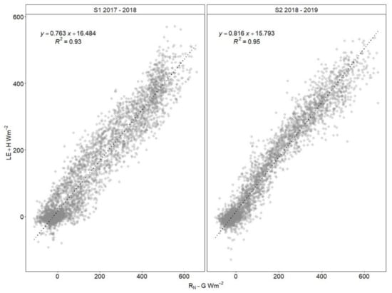
Figure 3.
Energy balance closure analysis based on 30 min averages during seasons S1 (November 2017–March 2018) and S2 (November 2018–March 2019). The dotted line is the regression line that describes the response of LE + H to RN-G changes.
Daily average fluxes (RN, H and λE) are shown in Figure 4. RN has lower values during early and late season, around 3 MJ m−2 day−1 in November and 10 MJ m−2day−1 in March and maximum values in December and January between 17 and 18 MJ m−2day−1, corresponding to flowering and development of fruits stages. The minimum values of λE are observed in both seasons in November (1.5–2.5 MJ m−2day−1) and March (2.3–1.9 MJ m−2day−1), while maximum values are observed in January in S1 (10.2 MJ m−2day−1) and in February in S2 (9.6 MJ m−2day−1). Hence, sensible heat flux (H) in both seasons shows higher values in December and February and lower in November and March. Thus, H is consistently higher than λE, representing 48% of RN, while λE represents 42% of RN.
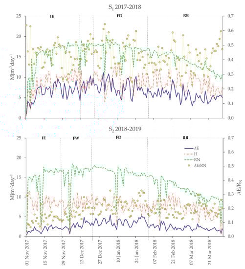
Figure 4.
Daily average energy balance components during seasons S1 (November 2017–March 2018) and S2 (November 2018–March 2019). Dashed lines indicate the duration of the following phenological phases of the vineyard: LD = Leaf Development (BBCH-11); IE = Inflorescence Emergence (BBCH-53); FW = Flowering (BBCH-61); DF = Development of Fruits (BBCH-71); RB = Ripening of Berries (BBCH-81).
Daily average fluxes (RN, H and λE) are shown in Figure 4. RN has lower values during early and late season, around 3 MJ m−2 day−1 in November and 10 MJ m−2day−1 in March and maximum values in December and January between 17 and 18 MJ m−2day−1, corresponding to flowering and development of fruits stages. The minimum values of λE are observed in both seasons in November (1.5–2.5 MJ m−2day−1) and March (2.3–1.9 MJ m−2day−1), while maximum values are observed in January in S1 (10.2 MJ m−2day−1) and in February in S2 (9.6 MJ m−2day−1). Hence, sensible heat flux (H) in both seasons shows higher values in December and February and lower in November and March. Thus, H is consistently higher than λE, representing 48% of RN, while λE represents 42% of RN.
The pattern of LAIEA per unit of ground area, estimated from measurements of radiation transmitted by the canopy is similar during S1 and S2 (Figure 5) with an initial phase of rapid growth between November and December, covering leaf development (LD) and inflorescence emergence (IE) stages, followed by a second phase where maximum values are reached during January and early February, including flowering (FW) and development of fruits (DF) stages, and finally a third phase where the LAIEA is slowly reduced from ripening of berries (RB) stage (Veraison) to the end of season (late February to April). Additionally, LAIEA values in S2 were lower than S1, mainly from flowering to ripening of berries stages, possibly due to canopy management that included higher frequency of pruning in S2.
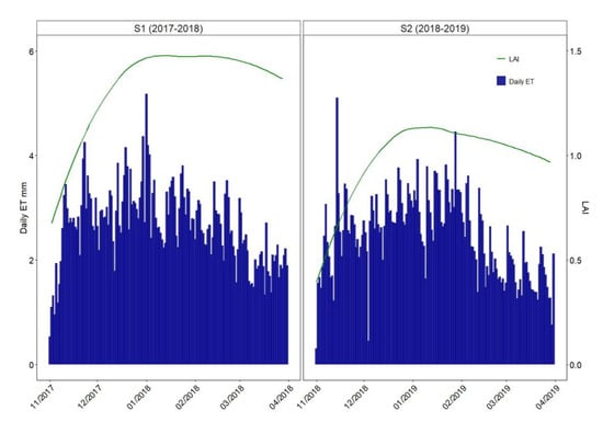
Figure 5.
Total daily evapotranspiration of the vineyard (Daily ET) and Leaf Area Index (LAIEA) during seasons S1 (November 2017–March 2018) and S2 (November 2018–March 2019).
3.2. Biophysical Variables Based on Remote Sensing Data
The NDVI–LAIEA regression analysis using Landsat 7–8 and Sentinel-2 data are shown in Figure 6a,b respectively. In both data sets the best fit were obtained using a power function with R2 values of 0.63 from Landsat 7–8 and 0.82 from Sentinel-2 data, suggesting that Sentinel-2 data provide better estimations of LAINDVI and canopy properties than Landsat 7–8 data.
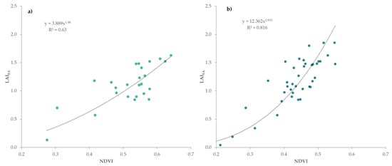
Figure 6.
Regression analysis between the adjusted leaf area index (LAIEA) and the normalized difference vegetation index (NDVI) estimated from Landsat 7–8 (a) and Sentinel-2 (b) data. The dotted line is the regression line that describes the response of LAIEA to NDVI changes.
Consequently, Figure 7a,b and Figure 8a,b show the seasonal pattern of LAINDVI from Landsat 7–8 and Sentinel-2 data, where seasonal bias (%Bias) is lower in Sentinel-2 (−2.8%) than Landsat 7–8 (−6.6%). On the other hand, LAINDVI values are lower in Landsat 7–8, with maximum around 1.4 m2 m−2 in both seasons, while in Sentinel-2 the maximum was around 2.1 m2 m−2 in S1 and 1.5 m2 m−2 in S2. However, despite the differences in magnitude and %Bias, in both data sets the pattern is similar, reproducing a three-phase trend.
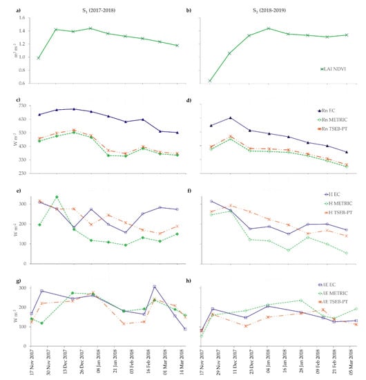
Figure 7.
Leaf area index and energy balance components involved in the measured and modeled instantaneous latent heat flux pattern during S1 (2017–2018) and S2 (2018–2019) in Landsat 7 and Landsat 8 satellite overpass time. (a,b) Leaf area index estimated from Landsat 7–8 (LAI NDVI) data in m2/m2. (c,d) Net radiation measured by eddy covariance (Rn EC) and modeled by METRIC (Rn METRIC) and TSEB-PT (Rn TSEB-PT). (e,f) Sensible heat flux measured by eddy covariance (H EC) and modeled by METRIC (H METRIC) and TSEB-PT (H TSEB-PT). (g,h) Latent heat flux measured by eddy covariance (λE EC) and modeled by METRIC (λE METRIC) and by TSEB-PT (λE TSEB-PT).

Figure 8.
Biophysical variables involved in latent heat flux patterns (λE) during seasons S1 (2017–2018) and S2 (2018–2019) in Sentinel-2 satellite overpass time. (a,b) Soil water content (SWC) in m3 m−3 and leaf area index estimated from Sentinel-2 data (LAI NDVI) in m2 m−2. (c,d) Instantaneous latent heat flux measured by eddy covariance (λE EC), modeled by Penman-Monteith–Leuning (λE RS-PML) and Penman-Monteith–Stewart (λE RS-PMS).
3.3. Assessment of Remote Sensing-Based ET Models
Linear regression analysis of the components of the energy balance (Figure 9), shows that modeled fluxes from RS-PMS and RS-PML are the most closely grouped around the 1:1 line. However, the RS-PMS model has the best fit of instantaneous sensible (H) and latent (λE) heat fluxes with R2 of 0.53 and 0.79, respectively. On the other hand, when comparing TIR-ET models, TSEB-PT gives the best fit of modeled λE with R2 of 0.6, while METRIC exhibits a low R2 of 0.3. However, comparing these models in terms of RMSE, %RMSE and d1 the difference between them is not so pronounced, having the TSEB-PT model a slightly better performance than METRIC with values of 55.5 Wm−2 (RMSE), 30.8% (%RMSE) and 0.64 (d1), versus 42.8 Wm−2 RMSE), 23.7% (%RMSE) and 0.62 (d1) yielded by TSEB-PT model (Table 5)
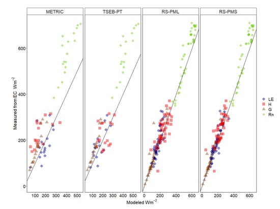
Figure 9.
Regression analysis and 1:1 line (solid line) between measured by eddy covariance (EC) and modeled energy balance components by Mapping Evapotranspiration at High Resolution with Internalized Calibration (METRIC), Priestley–Taylor Two Source Energy Balance (TSEB-PT), Remote Sensing Penman-Monteith–Leuning (RS-PML) and Remote Sensing Penman-Monteith–Stewart (RS-PMS).
Table 5.
Model comparison of estimations of evapotranspiration at different temporal scales.
Models based on the Penman-Monteith equation (RS-PML and RS-PMS) were evaluated with two approaches to estimate the soil evaporative fraction (fZhang and fSWC) as presented in equations 16 and 17 of Section 2.4.3. In this regard, for both RS-PML and RS-PMS the approach that includes soil water content measurements (fSWC) yielded the best goodness of fit in the estimation of instantaneous λE (Table 5), where a %RMSE of 21.3% (RS-PML) and 15.2% (RS-PMS), while fZhang approach results a %RMSE of 32.2% for RS-PML and 58.8% for RS-PMS (data not shown). Likewise, the Wilmott agreement index (d1) was higher under the fSWC approach (0.65–0.77) than the fZhang approach (0.52–0.33).
The seasonal pattern of λE modeled by the TIR-ET models and compared with λE measured by the eddy covariance (λE EC) (Figure 7), show that both METRIC and TSEB-PT replicate very well the intra-seasonal variability of λE EC, however, METRIC underestimates λE in S1 (−10.2 Wm−2) and overestimates in S2 (16.2 Wm−2), while TSEB-PT underestimates both seasons (−17.6 and 1–2.7 Wm−2). Therefore, Figure 7g,h show that METRIC tends to underestimate λE in early season (November-December), while the estimation is closer to measured λE between January and March. On the other hand, Figure 7g–h show that the TSEB-PT model underestimates λE when H is overestimated and, vice versa, λE is overestimated when H is overestimated, suggesting a strong dependence of λE with the remaining components of the energy balance, particularly H.
Assessing the intra-seasonal variation of λE modeled by RS-PML and RS-PMS (Figure 8c–d), both models successfully replicate the seasonal variability of λE, especially RS-PMS with a bias of −10.8 Wm−2 in S1 and −0.1 Wm−2 in S2, while RS-PML systematically underestimates in both seasons (−19.9 and −13.3 Wm−2).
4. Discussion
The results obtained at instantaneous time scale both METRIC and TSEB-PT are within the range of error reported in vineyards, with a RMSE ranging from 40 to 95 Wm−2 [21,90,91] in METRIC and from 47 to 89 Wm−2 in TSEB-PT model [28,30,92]. Additionally, both METRIC and TSEB-PT showed similar performance in terms of RMSE, %RMSE and d1. However, TSEB-PT had slightly better performance than METRIC (Table 5). This behavior may be due to both models sharing the same input data, as reported in an evaluation of both models in herbaceous (corn, soybean, wheat) and woody (olive and vineyards) crops [23].
The slight underestimation of TSEB-PT is possibly due to an overestimation of the short and long wave radiation components and hence a systematic underestimation of RN (Figure 7c,d), this implies less energy availability for the estimation of λE and H, especially if it is taken into account that λE is a residual function of the components of the energy balance [93,94]. Conversely, an underestimation of H implies greater energy availability for λE modeling and therefore its overestimation [93,95,96] as occurs in S2 with λE modeling by METRIC (Figure 7h).
Furthermore, LST estimation from Landsat-TIR bands require atmospheric and emissivity correction, which is a source of uncertainty in modeled H and consequently modeled λE from METRIC and TSEB-PT. However, METRIC reduces this uncertainty by including an internal calibration process, which depends on the selection of a hot (dry surface) and a cold (wet surface) pixel [15], selection done automatically throughout an exhaustive search algorithm [77]. On the other hand, TSEB-PT has greater sensitivity to LST estimation, since it is associated to estimation of TC, TAC and TS (Equations (10)–(12)) and consequently to the propagation of the error in H partition between soil (HS) and canopy (HC) [97].
When comparing approaches to model the soil evaporative fraction required both RS-PML and RS-PMS models, the best fit of the fSWC approach is because the energy for soil evaporation depends on the soil water content of top soil layers [41], which is captured by measuring the soil water content. However, satisfactory results have been obtained with the fZhang approach in sparsely vegetated areas characterized by a high evaporation rate and higher frequency of precipitation [44], which evidenced that the aforementioned approach reproduces well the dynamics of soil evaporation when it depends on the precipitation of previous days. Therefore, due to the characteristics of drip irrigation, where soil evaporation is located only in the portion of soil wetted by the dripper, the fSWC approach is able to simulate more accurately the soil evaporation dynamics under such conditions. The fSWC approach consistently had the best fit in comparison to the fZhang approach, hence hereinafter the results will be shown only for the fSWC approach for both the RS-PML and RS-PMS models, omitting the subscript fSWC.
Additionally, the results from the fSWC approach are comparable to those obtained in the evaluation of two remote sensing Penman-Monteith models (RS-PM) using visible, near-infrared and thermal infrared data from Landsat 5 and Landsat 7 platforms, yielding a higher RMSE around 39.7 Wm−2 and establishing the strong dependency between ET and soil water content, especially in irrigated vineyards and orchards, since a larger fraction of net radiation (RN) is allocated to instantaneous latent heat flux (λE) and not to instantaneous sensible heat flux (H), as would occur on dryland vegetation covers [39].
The behavior of λE modeled by RS-PML responds to phenology, to the error associated to LAI estimation (Figure 7a,b) from remote sensing data [41], to the inherent errors in λE measurement by the eddy covariance system and to the parameterization of the maximum stomatal conductance (gsx). The first two aspects were already discussed previously, while gsx is a species-specific parameter that varies according to phenology [41] and in this work is taken the maximum value reported in the bibliography [87]. In spite of the latter, it is possible that the selected gsx is lower than actually evidenced in the assessed seasons through measured λE, however, the gsx value satisfactorily represents the last phenological stage corresponding to Ripening of Berries (February–April) as is observed in Figure 7c,d where the bias is lower compared to the overall season.
On the other hand, the model of stomatal conductance developed by Stewart [45] provides a better description of transpiration dynamics in the vineyard, which involves the adjustment of four parameters (gSX, f1, f2 and f3), while the Leuning stomatal conductance approach [42] requires the adjustment of one parameter (gSX), becoming a model that can be easily applied in a wide range of environmental conditions. Additionally, the Stewart stomatal conductance model requires soil water content measurements, which are not commonly carried out in commercial vineyards, while the Leuning stomatal conductance model requires vapor pressure deficit measurements, which are available from nearby weather stations. However, SWC measurements in commercial fields should become more frequent since water restrictions for irrigation purposes are expected to increase in the coming years. Therefore, through the widespread adoption of SWC measurements, the monitoring of available water at the root zone would be improved and the application of the RS-PMS model would be extended to different environmental and agronomic management conditions.
Analyzing different timescales where instantaneous λE was extrapolated to daily ET, 7-day and monthly ET (Table 5), the best agreement index (d1) corresponds to the RS-PMS model (0.7), followed by RS-PML (0.58), TSEB-PT (0.56) and METRIC (0.5), which is consistent with respective RMSE and %RMSE values. Therefore, daily ET values modeled by METRIC have a slightly higher RMSE than those reported in vineyards [22,91,98], ranging from 0.4 to 0.8 mm day−1. These differences possibly are due to the extrapolation method chosen, since in addition to the approach used in this research (λE/Rs ratio), there are other common methods such as ET/ET0 [22,91] and ET/RN-G ratio [98].
In addition, daily ET error reported in vineyards by other TSEB models such as ALEXI/DisALEXI yield RMSE around 0.35–0.79 mm day−1 and %RMSE between 8 and 22% [28,30,99], which are lower than those obtained by TSEB-PT model, possibly due to the fusion of remote sensing data methodology used in ALEXI/DisALEXI models, allows a comprehensive daily characterization of vineyard water consumption.
Moreover, it is reported lower daily ET RMSE of 0.34 mm day−1 with RS-PM model that include brightness temperature data from satellite sensor [39], which improve modeled daily ET. However, both RS-PMS and RS-PML models are consistent with reported by the VIS-ET models based on multiple linear regression with RMSE around 0.62 mm day−1 [100].
The irrigation management in the evaluated vineyard takes as a criterion the ET0 multiplied by a crop coefficient (Kc) of 0.5 (ET0 × 0.5) during the whole season (Kc Target) (Figure 10c,d). In this context, the proposed RS-PMS model provides a method to evaluate and monitor whether the irrigation applied corresponds to the criteria selected. Therefore, Figure 9 shows the water irrigation applied in seasons S1 and S2, which is around to the estimated by the criterion ET0 × 0.5, despite irregular management in S1 (Figure 10a) in comparison with S2 (Figure 10b). Nonetheless, Figure 10c,d show that estimating the Kc provided by the eddy covariance system (Kc EC), which is the ratio between ET EC and ET0, has standard deviation of 0.04 and does not reach the Kc Target of 0.5, thus implying that the irrigation applied is lower than the estimated by the vineyard irrigation management. Hence, the Kc estimated by the RS-PMS model (Kc PMS), this means the ratio between ET RS-PMS and ET0, is reasonably similar to the Kc EC with a bias around 9% and standard deviation of 0.06, which would allow accurately the evaluation and monitoring of irrigation [101,102,103,104] at a spatial scale of 10 m × 10 m and a daily and weekly temporal scale, which are suitable for irrigation management.
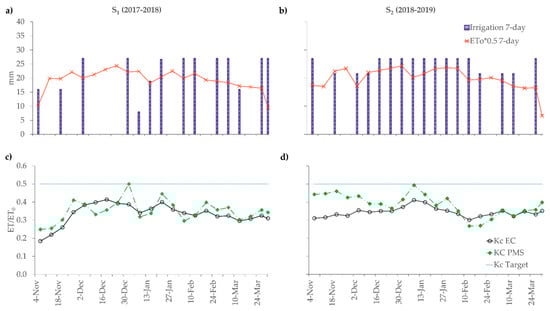
Figure 10.
(a,b) Irrigation schedule during S1 (2017–2018) (a) and S2 (2018–2019) (b) in 7-day cumulative intervals, total amount of water applied in mm (7-day irrigation) and total programmed irrigation in mm according to the criteria of crop coefficient (Kc) equal to 0.5 (ET0 × 5 7-day). (c,d) Comparison of the Kc = 0.5 (Kc Target) with the estimated Kc with data from both the eddy covariance system (Kc EC = ET EC/ETo) and the Penman-Monteith model for remote sensing coupled to Stewart’s stomatal conductance model (Kc PMS = ET PMS/ETo) during seasons S1 (c) and S2 (d).
Additionally, under the environmental conditions and vineyard management addressed in this study (Mediterranean climate and drip irrigation), RS-PMS outperforms RS-PML, METRIC and TSEB-PT. However, several researches have highlighted that TIR-ET methods are more appropriate than VIS-ET methods under conditions of water shortage, because LST is more sensitive to vegetation water condition, while VIS-ET methods do not have a fast response to early plant water stress [15,38]. In contrast, there are other studies that have concluded that VIS-ET models, with the current specifications of the available remote sensing platforms, have better performance than TIR-ET methods due to uncertainties in LST estimation for low pixel resolution (and widely separated row crops such as vineyards), impacting H estimation and generating uncertainties in λE, meanwhile VIS-ET models are capable to capture the heterogeneity of land surface, because of higher pixel resolution [13]. However, the data acquired by aircraft and Unmanned Airborne Vehicles (UAV) provide a high spatial resolution (<10 m) of TIR bands, reporting better fit of the actual evapotranspiration modeled by METRIC and TSEB-PT [20,29,31,105,106], which clearly suggests that the difference in performance of the TIR-ET and VIS-ET models is given by the resolution of the input data.
5. Conclusions
The Penman-Monteith model was evaluated for the estimation of actual evapotranspiration (ET) with remote sensing data (RS-PM) at multiple temporal scales, on a vineyard located in central Chile and under drip irrigation. Therefore, two approaches of the RS-PM model were evaluated, one based on the Leuning approach (RS-PML) [41] and a novel approach based on remote sensing data that couples the RS-PM model to Stewart’s stomatal conductance model [89] (RS-PMS). Both models employed Sentinel-2 remote sensing data and were compared with independent eddy covariance data and both the Mapping Evapotranspiration at High Resolution with Internalized Calibration (METRIC) [18] and the Priestley–Taylor Two-Source Energy Balance (TSEB-PT) [78], which are widely used to assess actual ET and are based on infrared thermal band data from the Landsat 7 and Landsat 8 satellites, with lower spatial and temporal resolution than the Sentinel-2 visible and near-infrared band data.
The RS-PM models outperform the METRIC and TSEB-PT models, especially in the instantaneous and daily time scales where RS-PM models have the lowest root mean square error (RMSE) and the highest Wilmott agreement index (d1). The higher temporal scale resolution of the input data in RS-PM models might be foremost responsible for those results since with higher resolution data obtained from aircraft and Unmanned Airborne Vehicles (UAV), both METRIC and TSEB-PT models performed similarly and even better than shown in this research for RS-PM models. On the other hand, the RS-PMS approach yields a better performance than RS-PML in all temporal scales evaluated, due to the four fitted parameters which improve the model ability to properly capture variations in soil water content, which in conjunction with the leaf area index determines the evapotranspiration rate of the vineyard managed with localized irrigation. However, the implementation of this approach under conditions different from those of this research will be subject to the availability of data to adjust the four model parameters, especially measurements of soil water content.
Finally, it was demonstrated that RS-PMS model is suitable to assess water consumption and irrigation management, since it is possible to estimate the actual Kc of the vineyard with the actual modeled ET (Kc PMS), which is one of the criteria used in irrigation management. Thus, on average the Kc PMS is biased by 9% compared to the Kc estimated with data from the Eddy covariance system (Kc EC). This is relevant taking into account it was found that during the two evaluated seasons, the vineyard’s Kc was bellow of the 0.5 target Kc, equivalent to 0.33 in S1 (2017–2018) and 0.34 in S2 (2018–2019), representing a 32% lower than planned.
Author Contributions
Conceptualization, V.G.-G. and F.J.M.; methodology, V.G.-G.; software, V.G.-G.; validation, V.G.-G., F.J.M., C.S. and P.M.G.; formal analysis, V.G.-G.; investigation, V.G.-G.; resources, F.J.M.; data curation, V.G.-G.; writing—original draft preparation, V.G.-G.; writing—review and editing, V.G.-G., F.J.M., C.S. and P.M.G.; visualization, V.G.-G.; supervision, F.J.M.; project administration, F.J.M.; funding acquisition, F.J.M. All authors have read and agreed to the published version of the manuscript.
Funding
This research was funded by FONDECYT, grant number 1170429 and partially supported by CONICYT REDES grant number 180025 and FONDEQUIP grant number EQM170024. Víctor García-Gutiérrez was financially supported by FONDECYT National Doctoral Grant number 21180457.
Institutional Review Board Statement
Not applicable.
Informed Consent Statement
Not applicable.
Data Availability Statement
The data presented in this study are available on request from the corresponding author. The data are not publicly available due to because it is currently being used in various research projects.
Acknowledgments
This work could not have been accomplished without the support from Pedro Ruiz-Tagle (vineyard landowner) and Pedro Mesina (vineyard manager).
Conflicts of Interest
The authors declare no conflict of interest.
References
- Arnell, N.W. Climate change and global water resources. Glob. Environ. Chang. 1999, 9 (Suppl. 1), S31–S49. [Google Scholar] [CrossRef]
- Boretti, A.; Rosa, L. Reassessing the projections of the World Water Development Report. Npj Clean Water 2019, 2, 15. [Google Scholar] [CrossRef]
- Kim, S.H.; Hejazi, M.; Liu, L.; Calvin, K.; Clarke, L.; Edmonds, J.; Kyle, P.; Patel, P.; Wise, M.; Davies, E. Balancing global water availability and use at basin scale in an integrated assessment model. Clim. Chang. 2016, 136, 217–231. [Google Scholar] [CrossRef]
- Schmied, H.M.; Adam, L.; Eisner, S.; Fink, G.; Flörke, M.; Kim, H.; Oki, T.; Portmann, F.T.; Reinecke, R.; Riedel, C.; et al. Variations of global and continental water balance components as impacted by climate forcing uncertainty and human water use. Hydrol. Earth Syst. Sci. 2016, 20, 2877–2898. [Google Scholar] [CrossRef]
- Wada, Y.; Flörke, M.; Hanasaki, N.; Eisner, S.; Fischer, G.; Tramberend, S.; Satoh, Y.; Van Vliet, M.T.H.; Yillia, P.; Ringler, C.; et al. Modeling global water use for the 21st century: The Water Futures and Solutions (WFaS) initiative and its approaches. Geosci. Model Dev. 2016, 9, 175–222. [Google Scholar] [CrossRef]
- Van Leeuwen, C.; Trégoat, O.; Choné, X.; Bois, B.; Pernet, D.; Gaudillère, J.-P. Vine water status is a key factor in grape ripening and vintage quality for red Bordeaux wine. How can it be assessed for vineyard management purposes? J. Int. Sci. Vigne Vin 2009, 43, 121–134. [Google Scholar] [CrossRef]
- Medrano, H.; Tomás, M.; Martorell, S.; Escalona, J.-M.; Pou, A.; Fuentes, S.; Flexas, J.; Bota, J. Improving water use efficiency of vineyards in semi-arid regions. A review. Agron. Sustain. Dev. 2015, 35, 499–517. [Google Scholar] [CrossRef]
- Munitz, S.; Schwartz, A.; Netzer, Y. Water consumption, crop coefficient and leaf area relations of a Vitis vinifera cv. “Cabernet Sauvignon” vineyard. Agric. Water Manag. 2019, 219, 86–94. [Google Scholar] [CrossRef]
- Romero, P.; Fernández-Fernández, J.I.; Ordaz, P.B. Interannual Climatic Variability Effects on Yield, Berry and Wine Quality Indices in Long-Term Deficit Irrigated Grapevines, Determined by Multivariate Analysis. Int. J. Wine Res. 2016, 8, 3–17. Available online: https://dialnet.unirioja.es/servlet/articulo?codigo=6846980&info=resumen&idioma=ENG (accessed on 26 October 2020).
- Serrano, L.; González-Flor, C.; Gorchs, G. Assessment of grape yield and composition using the reflectance based Water Index in Mediterranean rainfed vineyards. Remote Sens. Environ. 2012, 118, 249–258. [Google Scholar] [CrossRef]
- Anderson, M.C.; Allen, R.G.; Morse, A.; Kustas, W.P. Use of Landsat thermal imagery in monitoring evapotranspiration and managing water resources. Remote Sens. Environ. 2012, 122, 50–65. [Google Scholar] [CrossRef]
- Courault, D.; Seguin, B.; Olioso, A. Review on estimation of evapotranspiration from remote sensing data: From empirical to numerical modeling approaches. Irrig. Drain. Syst. 2005, 19, 223–249. [Google Scholar] [CrossRef]
- Glenn, E.P.; Nagler, P.; Huete, A. Vegetation Index Methods for Estimating Evapotranspiration by Remote Sensing. Surv. Geophys. 2010, 31, 531–555. [Google Scholar] [CrossRef]
- Glenn, E.P.; Huete, A.R.; Nagler, P.; Hirschboeck, K.K.; Brown, P. Integrating Remote Sensing and Ground Methods to Estimate Evapotranspiration. Crit. Rev. Plant Sci. 2007, 26, 139–168. [Google Scholar] [CrossRef]
- Gonzalez-Dugo, M.; Neale, C.; Mateos, L.; Kustas, W.; Prueger, J.; Anderson, M.; Li, F. A comparison of operational remote sensing-based models for estimating crop evapotranspiration. Agric. For. Meteorol. 2009, 149, 1843–1853. [Google Scholar] [CrossRef]
- Kustas, W.P.; Norman, J.M. Use of remote sensing for evapotranspiration monitoring over land surfaces. Hydrol. Sci. J. 1996, 41, 495–516. [Google Scholar] [CrossRef]
- Glenn, E.P.; Neale, C.M.U.; Hunsaker, D.; Nagler, P. Vegetation index-based crop coefficients to estimate evapotranspiration by remote sensing in agricultural and natural ecosystems. Hydrol. Process. 2011, 25, 4050–4062. [Google Scholar] [CrossRef]
- Allen, R.G.; Tasumi, M.; Trezza, R. Satellite-Based Energy Balance for Mapping Evapotranspiration with Internalized Calibration (METRIC)—Model. J. Irrig. Drain. Eng. 2007, 133, 380–394. [Google Scholar] [CrossRef]
- Long, D.; Singh, V.P. Assessing the impact of end-member selection on the accuracy of satellite-based spatial variability models for actual evapotranspiration estimation. Water Resour. Res. 2013, 49, 2601–2618. [Google Scholar] [CrossRef]
- Minacapilli, M.; Agnese, C.; Blanda, F.; Cammalleri, C.; Ciraolo, G.; D’Urso, G.; Iovino, M.; Pumo, D.; Provenzano, G.; Rallo, G. Estimation of actual evapotranspiration of Mediterranean perennial crops by means of remote-sensing based surface energy balance models. Hydrol. Earth Syst. Sci. 2009, 13, 1061–1074. [Google Scholar] [CrossRef]
- Carrasco-Benavides, M.; Ortega-Farias, S.; Lagos, O.; Kleissl, J.; Morales, L.; Kilic, A. Parameterization of the Satellite-Based Model (METRIC) for the Estimation of Instantaneous Surface Energy Balance Components over a Drip-Irrigated Vineyard. Remote Sens. 2014, 6, 11342–11371. [Google Scholar] [CrossRef]
- Carrasco-Benavides, M.; Ortega-Farias, S.; Lagos, L.O.; Kleissl, J.; Morales, L.; Poblete-Echeverría, C.; Allen, R.G. Crop coefficients and actual evapotranspiration of a drip-irrigated Merlot vineyard using multispectral satellite images. Irrig. Sci. 2012, 30, 485–497. [Google Scholar] [CrossRef]
- Guzinski, R.; Nieto, H.; Sandholt, I.; Karamitilios, G. Modelling High-Resolution Actual Evapotranspiration through Sentinel-2 and Sentinel-3 Data Fusion. Remote Sens. 2020, 12, 1433. [Google Scholar]
- Ciraolo, G.; Capodici, F.; D’Urso, G.; la Loggia, G.; Maltese, A. Mapping evapotranspiration on vineyards: The SENTINEL-2 potentiality-NASA/ADS. In Proceedings of the First Sentinel-2 Preparatory Symposium, Frascati, Italy, 23–27 April 2012. [Google Scholar]
- Galleguillos, M.; Jacob, F.; Prévot, L.; French, A.; Lagacherie, P. Comparison of two temperature differencing methods to estimate daily evapotranspiration over a Mediterranean vineyard watershed from ASTER data. Remote Sens. Environ. 2011, 115, 1326–1340. [Google Scholar] [CrossRef]
- Bisquert, M.; Sánchez, J.; López-Urrea, R.; Caselles, V. Estimating high resolution evapotranspiration from disaggregated thermal images. Remote Sens. Environ. 2016, 187, 423–433. [Google Scholar] [CrossRef]
- Parry, C.K.; Kustas, W.P.; Knipper, K.R.; Anderson, M.C.; Alfieri, J.G.; Prueger, J.H.; McElrone, A.J. Comparison of vineyard evapotranspiration estimates from surface renewal using measured and modelled energy balance components in the GRAPEX project. Irrig. Sci. 2019, 37, 333–343. [Google Scholar] [CrossRef]
- Knipper, K.; Kustas, W.P.; Anderson, M.C.; Alfieri, J.G.; Prueger, J.H.; Hain, C.R.; Gao, F.; Yang, Y.; McKee, L.G.; Nieto, H.; et al. Evapotranspiration estimates derived using thermal-based satellite remote sensing and data fusion for irrigation management in California vineyards. Irrig. Sci. 2018, 37, 431–449. [Google Scholar] [CrossRef]
- Nieto, H.; Bellvert, J.; Kustas, W.P.; Alfieri, J.G.; Gao, F.; Prueger, J.; Torres-Rua, A.F.; Hipps, L.E.; Elarab, M.; Song, L. Unmanned airborne thermal and mutilspectral imagery for estimating evapotranspiration in irrigated vineyards. In Proceedings of the International Geoscience and Remote Sensing Symposium (IGARSS), Fort Worth, TX, USA, 23–28 July 2017; pp. 5510–5513. [Google Scholar] [CrossRef]
- Semmens, K.A.; Anderson, M.C.; Kustas, W.P.; Gao, F.; Alfieri, J.G.; McKee, L.; Prueger, J.H.; Hain, C.R.; Cammalleri, C.; Yang, Y.; et al. Monitoring daily evapotranspiration over two California vineyards using Landsat 8 in a multi-sensor data fusion approach. Remote Sens. Environ. 2016, 185, 155–170. [Google Scholar] [CrossRef]
- Xia, T.; Kustas, W.P.; Anderson, M.C.; Alfieri, J.G.; Gao, F.; McKee, L.; Prueger, J.H.; Geli, H.M.E.; Neale, C.M.U.; Sanchez, L.; et al. Mapping evapotranspiration with high-resolution aircraft imagery over vineyards using one- and two-source modeling schemes. Hydrol. Earth Syst. Sci. 2016, 20, 1523–1545. [Google Scholar] [CrossRef]
- Allen, R.G.; Tasumi, M.; Morse, A.; Trezza, R. A Landsat-based energy balance and evapotranspiration model in Western US water rights regulation and planning. Irrig. Drain. Syst. 2005, 19, 251–268. [Google Scholar] [CrossRef]
- Senay, G.B.; Friedrichs, M.; Singh, R.K.; Velpuri, N.M. Evaluating Landsat 8 evapotranspiration for water use mapping in the Colorado River Basin. Remote Sens. Environ. 2016, 185, 171–185. [Google Scholar] [CrossRef]
- Vanino, S.; Nino, P.; De Michele, C.; Bolognesi, S.F.; D’Urso, G.; Di Bene, C.; Pennelli, B.; Vuolo, F.; Farina, R.; Pulighe, G.; et al. Capability of Sentinel-2 data for estimating maximum evapotranspiration and irrigation requirements for tomato crop in Central Italy. Remote Sens. Environ. 2018, 215, 452–470. [Google Scholar] [CrossRef]
- Rozenstein, O.; Haymann, N.; Kaplan, G.; Tanny, J. Estimating cotton water consumption using a time series of Sentinel-2 imagery. Agric. Water Manag. 2018, 207, 44–52. [Google Scholar] [CrossRef]
- Mokhtari, A.; Noory, H.; Pourshakouri, F.; Haghighatmehr, P.; Afrasiabian, Y.; Razavi, M.; Fereydooni, F.; Naeni, A.S. Calculating potential evapotranspiration and single crop coefficient based on energy balance equation using Landsat 8 and Sentinel-2. ISPRS J. Photogramm. Remote Sens. 2019, 154, 231–245. [Google Scholar] [CrossRef]
- Guzinski, R.; Nieto, H. Evaluating the feasibility of using Sentinel-2 and Sentinel-3 satellites for high-resolution evapotranspiration estimations. Remote Sens. Environ. 2019, 221, 157–172. [Google Scholar] [CrossRef]
- Vanino, S.; Pulighe, G.; Nino, P.; De Michele, C.; Bolognesi, S.F.; D’Urso, G. Estimation of Evapotranspiration and Crop Coefficients of Tendone Vineyards Using Multi-Sensor Remote Sensing Data in a Mediterranean Environment. Remote Sens. 2015, 7, 14708–14730. [Google Scholar] [CrossRef]
- Teixeira, A.H.D.C. Determining Regional Actual Evapotranspiration of Irrigated Crops and Natural Vegetation in the São Francisco River Basin (Brazil) Using Remote Sensing and Penman-Monteith Equation. Remote Sens. 2010, 2, 1287–1319. [Google Scholar] [CrossRef]
- Cleugh, H.A.; Leuning, R.; Mu, Q.; Running, S.W. Regional evaporation estimates from flux tower and MODIS satellite data. Remote Sens. Environ. 2007, 106, 285–304. [Google Scholar] [CrossRef]
- Leuning, R.; Zhang, Y.Q.; Rajaud, A.; Cleugh, H.; Tu, K. A simple surface conductance model to estimate regional evaporation using MODIS leaf area index and the Penman-Monteith equation. Water Resour. Res. 2008, 44, 10. [Google Scholar] [CrossRef]
- Leuning, R. A critical appraisal of a combined stomatal-photosynthesis model for C3 plants. Plant Cell Environ. 1995, 18, 339–355. [Google Scholar] [CrossRef]
- Morillas, L.; Leuning, R.; Villagarcía, L.; García, M.; Serrano-Ortiz, P.; Domingo, F. Improving evapotranspiration estimates in Mediterranean drylands: The role of soil evaporation. Water Resour. Res. 2013, 49, 6572–6586. [Google Scholar] [CrossRef]
- Zhang, Y.; Leuning, R.; Hutley, L.B.; Beringer, J.; McHugh, I.; Walker, J.P. Using long-term water balances to parameterize surface conductances and calculate evaporation at 0.05° spatial resolution. Water Resour. Res. 2010, 46, 5512. [Google Scholar] [CrossRef]
- Stewart, J. Modelling surface conductance of pine forest. Agric. For. Meteorol. 1988, 43, 19–35. [Google Scholar] [CrossRef]
- Baldocchi, D.D. Assessing the eddy covariance technique for evaluating carbon dioxide exchange rates of ecosystems: Past, present and future. Glob. Chang. Biol. 2003, 9, 479–492. [Google Scholar] [CrossRef]
- Vickers, D.; Mahrt, L.; Vickers, D.; Mahrt, L. Quality Control and Flux Sampling Problems for Tower and Aircraft Data. J. Atmos. Ocean. Technol. 1997, 14, 512–526. [Google Scholar] [CrossRef]
- Wilczak, J.M.; Oncley, S.P.; Stage, S.A. Sonic Anemometer Tilt Correction Algorithms. Bound. Layer Meteorol. 2001, 99, 127–150. [Google Scholar] [CrossRef]
- Kaimal, J.C.; Finnigan, J.J. Atmospheric Boundary Layer Flows: Their Structure and Measurement; Oxford University Press: Bracknell, UK; Berks, UK, 1994. [Google Scholar]
- Moncrieff, J.; Massheder, J.; De Bruin, H.; Elbers, J.; Friborg, T.; Heusinkveld, B.; Kabat, P.; Scott, S.; Soegaard, H.; Verhoef, A. A system to measure surface fluxes of momentum, sensible heat, water vapour and carbon dioxide. J. Hydrol. 1997, 188–189, 589–611. [Google Scholar] [CrossRef]
- Webb, E.K.; Pearman, G.I.; Leuning, R. Correction of flux measurements for density effects due to heat and water vapour transfer. Q. J. R. Meteorol. Soc. 1980, 106, 85–100. [Google Scholar] [CrossRef]
- Foken, T.; Wichura, B. Tools for quality assessment of surface-based flux measurements. Agric. For. Meteorol. 1996, 78, 83–105. [Google Scholar] [CrossRef]
- Wilson, K.; Goldstein, A.; Falge, E.; Aubinet, M.; Baldocchi, D.; Berbigier, P.; Bernhofer, C.; Ceulemans, R.; Dolman, A.; Field, C.; et al. Energy balance closure at FLUXNET sites. Agric. For. Meteorol. 2002, 113, 223–243. [Google Scholar] [CrossRef]
- Kljun, N.; Calanca, P.; Rotach, M.W.; Schmid, H.P. A Simple Parameterisation for Flux Footprint Predictions. Bound. Layer Meteorol. 2004, 112, 503–523. [Google Scholar] [CrossRef]
- Barcza, Z.; Kern, A.; Haszpra, L.; Kljun, N. Spatial representativeness of tall tower eddy covariance measurements using remote sensing and footprint analysis. Agric. For. Meteorol. 2009, 149, 795–807. [Google Scholar] [CrossRef]
- Chen, B.; Black, T.A.; Coops, N.C.; Hilker, T.; Trofymow, J.A. (Tony); Morgenstern, K. Assessing Tower Flux Footprint Climatology and Scaling Between Remotely Sensed and Eddy Covariance Measurements. Bound. Layer Meteorol. 2008, 130, 137–167. [Google Scholar] [CrossRef]
- Bai, J.; Jia, L.; Liu, S.M.; Xu, Z.; Hu, G.; Zhu, M.; Song, L. Characterizing the Footprint of Eddy Covariance System and Large Aperture Scintillometer Measurements to Validate Satellite-Based Surface Fluxes. IEEE Geosci. Remote Sens. Lett. 2015, 12, 943–947. [Google Scholar] [CrossRef]
- Lorenz, D.; Eichhorn, K.; Bleiholder, H.; Klose, R.; Meier, U.; Weber, E. Growth Stages of the Grapevine: Phenological growth stages of the grapevine (Vitis vinifera L. ssp. vinifera)—Codes and descriptions according to the extended BBCH scale. Aust. J. Grape Wine Res. 1995, 1, 100–103. [Google Scholar] [CrossRef]
- Bellan, M.; Marková, I.; Zaika, A.; Krejza, J. Light use efficiency of aboveground biomass production of Norway spruce stands. Acta Univ. Agric. Silvic. Mendel. Brun. 2017, 65, 9–16. [Google Scholar] [CrossRef]
- Černý, J.; Krejza, J.; Pokorný, R.; Bednář, P. LaiPen LP 100–a new device for estimating forest ecosystem leaf area index compared to the etalon: A methodologic case study. J. For. Sci. 2018, 64, 455–468. [Google Scholar] [CrossRef]
- Homolová, L.; Janoutová, R.; Lukeš, P.; Hanuš, J.; Novotný, J.; Brovkina, O.; Fernandez, R.R.L. In situ data supporting remote sensing estimation of spruce forest parameters at the ecosystem station Bílý Kříž. Beskydy 2017, 10, 75–86. [Google Scholar] [CrossRef]
- Monsi, M.; Saeki, T. On the Factor Light in Plant Communities and its Importance for Matter Production. Ann. Bot. 2004, 95, 549–567. [Google Scholar] [CrossRef]
- Ortega-Farias, S.; Carrasco, M.; Olioso, A.; Acevedo, C.; Poblete, C. Latent heat flux over Cabernet Sauvignon vineyard using the Shuttleworth and Wallace model. Irrig. Sci. 2006, 25, 161–170. [Google Scholar] [CrossRef]
- Patakas, A.; Noitsakis, B. An indirect method of estimating leaf area index in cordon trained spur pruned grapevines. Sci. Hortic. 1999, 80, 299–305. [Google Scholar] [CrossRef]
- Lopez-Lozano, R.; Baret, F.; De Cortazar-Atauri, I.G.; Bertrand, N.; Casterad, M.A. Optimal geometric configuration and algorithms for LAI indirect estimates under row canopies: The case of vineyards. Agric. For. Meteorol. 2009, 149, 1307–1316. [Google Scholar] [CrossRef]
- Roy, D.P.; Wulder, M.; Loveland, T.R.; Woodcock, C.; Allen, R.; Anderson, M.; Helder, D.; Irons, J.; Johnson, D.; Kennedy, R.; et al. Landsat-8: Science and product vision for terrestrial global change research. Remote Sens. Environ. 2014, 145, 154–172. [Google Scholar] [CrossRef]
- Drusch, M.; Del Bello, U.; Carlier, S.; Colin, O.; Fernandez, V.M.; Gascon, F.; Hoersch, B.; Isola, C.; Laberinti, P.; Martimort, P.; et al. Sentinel-2: ESA’s Optical High-Resolution Mission for GMES Operational Services. Remote Sens. Environ. 2012, 120, 25–36. [Google Scholar] [CrossRef]
- Savitzky, A.; GolayE, M.J. Smoothing and Differentiation of Data by Simplified Least Squares Procedures. Anal. Chem. 1964, 36, 1627–1639. Available online: https://pubs.acs.org/sharingguidelines (accessed on 23 December 2020). [CrossRef]
- Anderson, M.C.; Norman, J.M.; Kustas, W.P.; Li, F.; Prueger, J.H.; Mecikalski, J.R. Effects of Vegetation Clumping on Two–Source Model Estimates of Surface Energy Fluxes from an Agricultural Landscape during SMACEX. J. Hydrometeorol. 2005, 6, 892–909. [Google Scholar] [CrossRef]
- Jimenez-Munoz, J.; Cristobal, J.; Sobrino, J.; Soria, G.; Ninyerola, M.; Pons, X. Revision of the Single-Channel Algorithm for Land Surface Temperature Retrieval From Landsat Thermal-Infrared Data. IEEE Trans. Geosci. Remote Sens. 2009, 47, 339–349. [Google Scholar] [CrossRef]
- Jimenez-Munoz, J.C.; Sobrino, J.A.; Jovanovic, D.S.; Mattar, C.; Cristobal, J. Land Surface Temperature Retrieval Methods From Landsat-8 Thermal Infrared Sensor Data. IEEE Geosci. Remote Sens. Lett. 2014, 11, 1840–1843. [Google Scholar] [CrossRef]
- Kalnay, E.; Kanamitsu, M.; Kistler, R.; Collins, W.; Deaven, D.; Gandin, L.; Iredell, M.; Saha, S.; White, G.; Woollen, J.; et al. The NCEP/NCAR 40-Year Reanalysis Project. Bull. Am. Meteorol. Soc. 1996, 77, 437–472. [Google Scholar] [CrossRef]
- Gorelick, N.; Hancher, M.; Dixon, M.; Ilyushchenko, S.; Thau, D.; Moore, R. Google Earth Engine: Planetary-scale geospatial analysis for everyone. Remote Sens. Environ. 2017, 202, 18–27. [Google Scholar] [CrossRef]
- Ma, Y.; Liu, S.M.; Song, L.; Xu, Z.; Liu, Y.; Xu, T.; Zhu, Z. Estimation of daily evapotranspiration and irrigation water efficiency at a Landsat-like scale for an arid irrigation area using multi-source remote sensing data. Remote Sens. Environ. 2018, 216, 715–734. [Google Scholar] [CrossRef]
- Kustas, W.P.; Norman, J.M. Evaluation of soil and vegetation heat flux predictions using a simple two-source model with radiometric temperatures for partial canopy cover. Agric. For. Meteorol. 1999, 94, 13–29. [Google Scholar] [CrossRef]
- Tasumi, M. Estimating evapotranspiration using METRIC model and Landsat data for better understandings of regional hydrology in the western Urmia Lake Basin. Agric. Water Manag. 2019, 226, 105805. [Google Scholar] [CrossRef]
- Bhattarai, N.; Quackenbush, L.J.; Im, J.; Shaw, S.B. A new optimized algorithm for automating endmember pixel selection in the SEBAL and METRIC models. Remote Sens. Environ. 2017, 196, 178–192. [Google Scholar] [CrossRef]
- Kustas, W.P.; Norman, J.M. A Two-Source Energy Balance Approach Using Directional Radiometric Temperature Observations for Sparse Canopy Covered Surfaces. Agron. J. 2000, 92, 847–854. [Google Scholar] [CrossRef]
- Nieto, H.; Kustas, W.P.; Torres-Rúa, A.; Alfieri, J.G.; Gao, F.; Anderson, M.C.; White, W.A.; Song, L.; Alsina, M.M.; Prueger, J.H.; et al. Evaluation of TSEB turbulent fluxes using different methods for the retrieval of soil and canopy component temperatures from UAV thermal and multispectral imagery. Irrig. Sci. 2018, 37, 389–406. [Google Scholar] [CrossRef]
- Norman, J.; Kustas, W.; Humes, K. Source approach for estimating soil and vegetation energy fluxes in observations of directional radiometric surface temperature. Agric. For. Meteorol. 1995, 77, 263–293. [Google Scholar] [CrossRef]
- Priestley, C.H.B.; Taylor, R.J. On the Assessment of Surface Heat Flux and Evaporation Using Large-Scale Parameters. Mon. Weather Rev. 1972, 100, 81–92. [Google Scholar] [CrossRef]
- Bonafoni, S.; Sekertekin, A. Albedo Retrieval From Sentinel-2 by New Narrow-to-Broadband Conversion Coefficients. IEEE Geosci. Remote Sens. Lett. 2020, 17, 1618–1622. [Google Scholar] [CrossRef]
- Idso, S.B.; Jackson, R.D. Thermal radiation from the atmosphere. J. Geophys. Res. Space Phys. 1969, 74, 5397–5403. [Google Scholar] [CrossRef]
- Soliman, A.S.; Heck, R.J.; Brenning, A.; Brown, R.; Miller, S. Remote Sensing of Soil Moisture in Vineyards Using Airborne and Ground-Based Thermal Inertia Data. Remote Sens. 2013, 5, 3729–3748. [Google Scholar] [CrossRef]
- Leuning, R.; Kelliher, F.M.; Pury, D.G.G.; Schulze, E.-D. Leaf nitrogen, photosynthesis, conductance and transpiration: Scaling from leaves to canopies. Plant Cell Environ. 1995, 18, 1183–1200. [Google Scholar] [CrossRef]
- Winkel, T.; Rambal, S. Stomatal conductance of some grapevines growing in the field under a Mediterranean environment. Agric. For. Meteorol. 1990, 51, 107–121. [Google Scholar] [CrossRef]
- Jara-Rojas, F.; Ortega-Farias, S.; Valdés-Gómez, H.; Poblete, C.; Del Pozo, A. Model Validation for Estimating the Leaf Stomatal Conductance in cv. Cabernet Sauvignon Grapevines. Chil. J. Agric. Res. 2009, 69, 88–96. [Google Scholar] [CrossRef]
- Green, S.; Clothier, B.; van den Dijssel, C.; Deurer, M.; Davidson, P.; Ahuja, L.R.; Reddy, V.R.; Saseendran, S.A.; Yu, Q. Measuring and modeling the stress response of grapevines to soil-water deficits. In Response of Crops to Limited Water: Understanding and Modeling Water Stress Effects on Plant Growth Processes; Advancesinagric, Responseofcrops, American Society of Agronomy, Crop Science Society of America, Soil Science Society of America: New York, NY, USA, 2008; pp. 357–385. [Google Scholar]
- Willmott, C.J. On the validation of models. Phys. Geogr. 1981, 2, 184–194. [Google Scholar] [CrossRef]
- De La Fuente-Sáiz, D.; Ortega-Farías, S.; Fonseca, D.; Ortega-Salazar, S.; Kilic, A.; Allen, R.G. Calibration of METRIC Model to Estimate Energy Balance over a Drip-Irrigated Apple Orchard. Remote Sens. 2017, 9, 670. [Google Scholar] [CrossRef]
- Gonzalez-Piqueras, J.; Carrilero, J.V.; Balbontín, C. Seguimiento de los flujos de calor sensible y calor latente en vid mediante la aplicación del balance de energía METRIC. Rev. Teledetección 2015, 43, 43–54. [Google Scholar] [CrossRef]
- González-Dugo, M.P.; González-Piqueras, J.; Campos, I.; Andréu, A.; Balbontín, C.; Calera, A. Evapotranspiration monitoring in a vineyard using satellite-based thermal remote sensing. In Remote Sensing for Agriculture, Ecosystems, and Hydrology XIV; SPIE: Edinburgh, UK, 2012; p. 8531. [Google Scholar] [CrossRef]
- Reyes-González, A.; Kjaersgaard, J.; Trooien, T.; Reta-Sánchez, D.G.; Sánchez-Duarte, J.I.; Preciado-Rangel, P.; Hernández, M.F. Comparison of Leaf Area Index, Surface Temperature, and Actual Evapotranspiration Estimated Using the METRIC Model and In Situ Measurements. Sensors 2019, 19, 1857. [Google Scholar] [CrossRef]
- Tang, R.; Li, Z.-L.; Jia, Y.; Li, C.; Chen, K.-S.; Sun, X.; Lou, J. Evaluating one- and two-source energy balance models in estimating surface evapotranspiration from Landsat-derived surface temperature and field measurements. Int. J. Remote Sens. 2012, 34, 3299–3313. [Google Scholar] [CrossRef]
- French, A.N.; Hunsaker, D.; Thorp, K.R. Remote sensing of evapotranspiration over cotton using the TSEB and METRIC energy balance models. Remote Sens. Environ. 2015, 158, 281–294. [Google Scholar] [CrossRef]
- Kilic, A.; Allen, R.; Trezza, R.; Ratcliffe, I.; Kamble, B.; Robison, C.; Ozturk, D. Sensitivity of evapotranspiration retrievals from the METRIC processing algorithm to improved radiometric resolution of Landsat 8 thermal data and to calibration bias in Landsat 7 and 8 surface temperature. Remote Sens. Environ. 2016, 185, 198–209. [Google Scholar] [CrossRef]
- Zhao, P.; Zhang, X.; Li, S.; Kang, S. Vineyard Energy Partitioning Between Canopy and Soil Surface: Dynamics and Biophysical Controls. J. Hydrometeorol. 2017, 18, 1809–1829. [Google Scholar] [CrossRef]
- Paço, T.A.; Pôças, I.; Cunha, M.; Silvestre, J.C.; Santos, F.L.; Paredes, P.; Pereira, L.S. Evapotranspiration and crop coefficients for a super intensive olive orchard. An application of SIMDualKc and METRIC models using ground and satellite observations. J. Hydrol. 2014, 519, 2067–2080. [Google Scholar] [CrossRef]
- Kustas, W.P.; Alfieri, J.G.; Nieto, H.; Wilson, T.G.; Gao, F.; Anderson, M.C. Utility of the two-source energy balance (TSEB) model in vine and interrow flux partitioning over the growing season. Irrig. Sci. 2018, 37, 375–388. [Google Scholar] [CrossRef]
- Dold, C.; Heitman, J.; Giese, G.; Howard, A.; Havlin, J.; Sauer, T. Upscaling Evapotranspiration with Parsimonious Models in a North Carolina Vineyard. Agronomy 2019, 9, 152. [Google Scholar] [CrossRef]
- Campos, I.; Neale, C.M.; Calera, A.; Balbontín, C.; González-Piqueras, J. Assessing satellite-based basal crop coefficients for irrigated grapes (Vitis vinifera L.). Agric. Water Manag. 2010, 98, 45–54. [Google Scholar] [CrossRef]
- Balbontín, C.; Campos, I.; Odi-Lara, M.; Ibacache, A.; Calera, A. Irrigation Performance Assessment in Table Grape Using the Reflectance-Based Crop Coefficient. Remote Sens. 2017, 9, 1276. [Google Scholar] [CrossRef]
- Tasumi, M.; Allen, R.G.; Trezza, R.; Wright, J.L. Satellite-Based Energy Balance to Assess Within-Population Variance of Crop Coefficient Curves. J. Irrig. Drain. Eng. 2005, 131, 94–109. [Google Scholar] [CrossRef]
- Picón-Toro, J.; González-Dugo, V.; Uriarte, D.; Mancha, L.A.; Testi, L. Effects of canopy size and water stress over the crop coefficient of a “Tempranillo” vineyard in south-western Spain. Irrig. Sci. 2012, 30, 419–432. [Google Scholar] [CrossRef]
- Chen, A.; Orlov-Levin, V.; Meron, M. Applying high-resolution visible-channel aerial imaging of crop canopy to precision irrigation management. Agric. Water Manag. 2019, 216, 196–205. [Google Scholar] [CrossRef]
- Khaliq, A.; Comba, L.; Biglia, A.; Aimonino, D.R.; Chiaberge, M.; Gay, P. Comparison of Satellite and UAV-Based Multispectral Imagery for Vineyard Variability Assessment. Remote Sens. 2019, 11, 436. [Google Scholar] [CrossRef]
Publisher’s Note: MDPI stays neutral with regard to jurisdictional claims in published maps and institutional affiliations. |
© 2021 by the authors. Licensee MDPI, Basel, Switzerland. This article is an open access article distributed under the terms and conditions of the Creative Commons Attribution (CC BY) license (http://creativecommons.org/licenses/by/4.0/).