Spatiotemporal Variability in the Glacier Snowline Altitude across High Mountain Asia and Potential Driving Factors

Abstract

The glacier snowline altitude (SLA) at the end of the melt season is an indicator of the glacier equilibrium line altitude and can be used to estimate glacier mass balance and reconstruct past climate. This study analyzes the spatiotemporal variability in glacier SLA across High Mountain Asia, including the Altai Mountains, Karakoram Mountains, Western Himalayas, Gongga Mountains, Tian Shan, and Nyainqentanglha Mountains, over the past 30 years (1989–2019) to better elucidate the state of these mountain glaciers. Remote-sensing data are processed to delineate the glacier SLA across these mountainous regions, and nearby weather station data are incorporated to determine the potential relationships between SLA and temperature/precipitation. The mean SLAs across the Altai and Karakoram mountains ranged from 2860 ± 169 m to 3200 ± 152 m and from 5120 ± 159 m to 5320 ± 240 m, respectively, with both regions experiencing an average increase of up to 137 m over the past 30 years. Furthermore, the mean glacier SLAs across the Western Himalayas and Gongga Mountains increased by 190–282 m over the past 30 years, with both regions experiencing large fluctuations. In particular, the mean glacier SLA across the Western Himalayas varied from 4910 ± 190 m in 1989 to 5380 ± 164 m in 2000, and that across the Gongga Mountains varied from 4960 ± 70 m in 1989 to 5330 ± 100 m in 2012. Correlation analyses between glacier SLA and temperature/precipitation suggest that temperature is the primary factor influencing glacier SLA across these High Mountain Asia glaciers. There is a broad increase in glacier SLA from the Altai Mountains to the Karakoram Mountains, with a decrease in glacier SLA with decreasing latitude across the Himalayas; the maximum SLA occurs near the northern slopes of the Western Himalayas. The glacier SLA is lower on the eastern side of the Tibetan Plateau and exhibits a longitudinal distribution pattern. These results are expected to provide useful information for evaluating the state of High Mountain Asia glaciers, as well as their response and feedback to climate change.

1. Introduction

Mountain glacier is a critical component of the Earth’s system, and its serve as a key freshwater source in many regions [1]. Glacier changes also have a significant impact on sea level [2]. Moreover, they can also lead to devastating natural disasters, including outburst glacier floods and glacier debris flow [3]. Changes in mountain glaciers also serve as a primary indicator of climate change. Glacier variation can be determined by monitoring changes in glacier area, length, mass balance, equilibrium line altitude (ELA, the ELA is a line on the glacier where annual accumulation equals ablation) or snowline altitude (SLA), and the contribution of global mountain glaciers and small ice caps to sea-level rise can be estimated through mass balance calculation [4]. Observations of glacier/snow parameters (e.g., mass balance and ELA) from a large mountain range and/or cryospheric region can assist to identify the influence of meteorological parameters (e.g., temperature and precipitation) on glacier changes for a region of interest, and promote better understanding of the relationship between glaciers and the climate at a regional scale. In particular, the ELA of glaciers can be used to determine the transient accumulation area ratio (AAR) and further estimate the mass balance of glaciers [5,6,7]. However, mass balance monitoring in general requires substantial financial and technical support to conduct ground-based observations, and thus it is difficult obtain mass balance data covering a large regions due to the limited number of ground observation sites. Paterson [8] indicated that the SLA at the end of the melt season is approximately equal to the ELA. Therefore, SLA has been used to represent ELA in mid-latitude glaciers [6,9,10,11].

Remote sensing is a powerful tool to monitor the evolution of glacial systems, due to its high temporal-spatial resolution and coverage, and is particularly useful to map SLA of glaciers where ground-based observations and/or regional-scale constraints are rare [12]. To discern SLA from remote sensing data, analysts first need to extract the snow boundary or area [13,14], then distinguish the boundary between snow and ice, and finally, a digital elevation model (DEM) is used to determine SLA [15,16]. This SLA recognition procedure utilizes different data processing methods, including the band combination method [17,18], the band ratio method [9,13] and the threshold method [19,20]. Extant literatures have also used MODIS data to determine regional SLA in the Tibetan Plateau and its environs [21,22,23,24]. However, the research results on glacial changes in High Mountain Asia so far are still quite scarce. In particular, High Mountain Asia glaciers are critical for both the global water cycle and water eco-environment in the arid regions of central Asia. Therefore, in this paper, the quantitative method based on the difference between snow and ice albedo determines a single glacier SLA.

In this study, we present remote sensing data covering High Mountain Asia, where the SLA of different glaciers and there changes over the past ~20 years are identified. The resultant SLA data are then compared with local meteorological data including summer mean temperature and precipitation, in order to explore the potential influence of weather and/or climate conditions on SLA changes. The results are expected to provide information that is useful to evaluate the state of High Mountain Asia glaciers and their response and feedback to climate change.

2. Study Site

High Mountain Asia (27–50°N, 70–105°E) comprises the Tibetan Plateau and surrounding Asian mountain ranges and possesses the largest cryosphere environment outside of the Polar Regions (Figure 1). They are bounded by the Altai Mountains to the north, the Himalayas to the south, the Pamir Mountains and the Western Tian Shan to the west, and the Qilian Mountains and the Hengduan Mountains to the east. There are 97,974 modern glaciers across this region, covering a vast area of 98,768.86 km² with ice storage of 1.1 × 10⁴ to 1.5 × 10⁴ km³, and producing 110–150 km³ melt water annually [25].

The western and northern regions of High Mountain Asia are affected primarily by the westerlies, whereas the southwest region is affected mainly by the Indian monsoon. The eastern and southeastern regions are influenced mainly by the East Asian monsoon and also by the plateau monsoon caused by the uplift of the Tibetan Plateau [26,27]. Owing to the impact of different wind systems, High Mountain Asia regional glaciers can be catalogued as continental or marine glaciers in the southwest and continental or polar glaciers in the northwest [26,28]. Annual precipitation ranges from 600 to 1000 mm in the Altai Mountains to above 3000 mm in the southeast region of High Mountain Asia. Precipitation is the material basis of mass balance and ELA changes. Accordingly, glacier ELAs vary from 2800 m in the Altai Mountains to 6200 m in the Himalayas [29].

Temporal variations in SLA were investigated by selecting subsets of representative glaciers in both the monsoon and westerlies regions of High Mountain Asia. Glaciers from the Altai Mountains (6) and the Karakoram Mountains (9) were chosen to represent the westerlies region, and glaciers from the Western Himalayas (12) and the Gongga Mountains (5) were chosen to represent the monsoon region. The locations of the selected glaciers are listed in Figure 1.

3. Data and Methods

3.1. Data

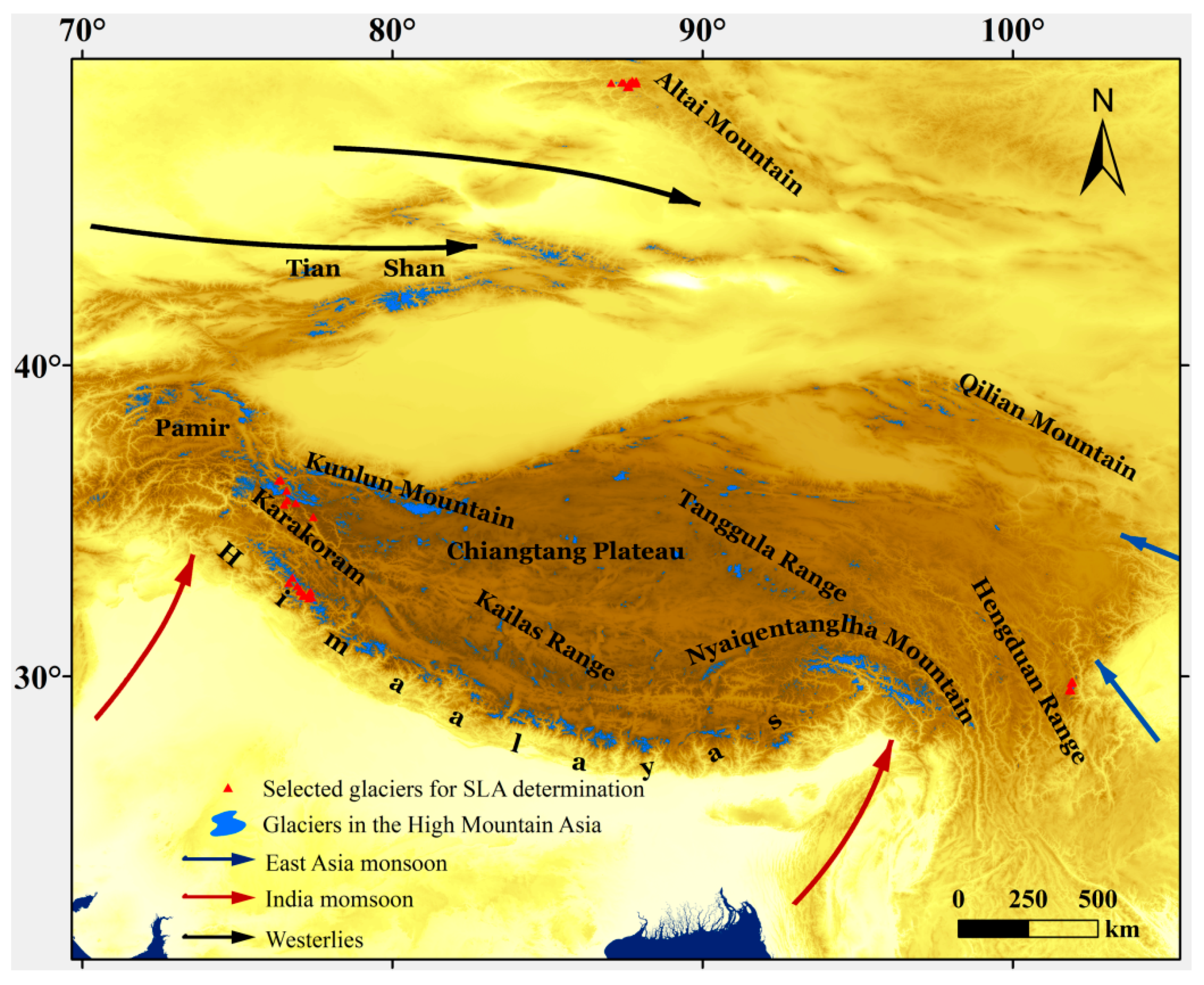
Landsat Multispectral Scanner System (MSS)/Thematic Mapper ™/Enhanced Thematic Mapper Plus (ETM+)/Operational Land Imager (OLI) data were downloaded from the USGS (http://earthexplorer.usgs.gov/) and the Geospatial Data Cloud (http://www.gscloud.cn). According to the three criteria for image selection, Landsat images of the Altai Mountains, the Karakoram Mountains, the Himalayas, and the Gongga Mountain from 1989 to 2019 were screened (

Table 1. Landsat MSS/TM/ETM+/OLI data used for mapping SLA.

Study Region	Path/Row	Sensor	Date	Data Source
The Altai Mountains	144/26	MSS	1989/8/17	USGS
		TM5	1993/8/12	USGS
		TM5	1996/8/20	USGS
		TM5	1998/8/26	USGS
		ETM+	2000/8/7	GSCloud
		ETM+	2001/8/10	USGS
		ETM+	2004/8/18	GSCloud
		ETM+	2006/7/23	GSCloud
		TM5	2007/8/3	USGS
		ETM+	2008/8/13	GSCloud
		TM5	2009/8/8	GSCloud
		TM5	2010/8/27	GSCloud
		ETM+	2012/8/24	GSCloud
		ETM+	2013/8/27	USGS
		OLI	2015/7/24	GSCloud
		OLI	2016/8/25	GSCloud
		OLI	2017/8/14	USGS
		OLI	2019/8/4	USGS
The Karakoram Mountains	148/35	TM 5	1991/8/19	USGS
		TM5	1993/7/7	USGS
		TM5	1994/7/26	USGS
		TM5	1996/8/16	USGS
		TM5	1997/7/18	USGS
		TM5	1999/8/9	USGS
		TM5	2000/8/27	USGS
		ETM+	2001/7/21	USGS
		ETM+	2002/8/9	USGS
		ETM+	2004/8/14	USGS
		ETM+	2005/9/2	USGS
		ETM+	2006/8/20	USGS
		ETM+	2007/8/23	USGS
		ETM+	2009/8/12	USGS
		ETM+	2010/8/31	USGS
		TM5	2011/8/10	GSCloud
		OLI	2013/7/30	USGS
		ETM+	2014/7/25	USGS
		OLI	2015/8/21	USGS
		ETM+	2017/8/18	USGS
		ETM+	2018/8/21	USGS
		OLI	2019/8/16	USGS
The Himalayas	147/37	TM5	1989/8/6	USGS
		TM5	1991/8/28	USGS
		TM5	1992/8/14	USGS
		TM5	1993/9/2	USGS
		TM5	1994/8/20	USGS
		TM5	1998/8/31	USGS
		ETM+	2000/8/28	GSCloud
		ETM+	2002/8/2	GSCloud
		ETM+	2004/9/8	USGS
		ETM+	2007/8/16	USGS
		TM 5	2009/8/13	USGS
		ETM+	2011/9/12	USGS
		OLI	2013/7/23	GSCloud
		OLI	2014/8/11	USGS
		OLI	2015/9/15	GSCloud
		OLI	2016/8/16	USGS
		OLI	2018/8/22	USGS
The Gongga Mountains	131/39	TM5	1989/6/19	USGS
		TM5	1990/7/8	USGS
		TM5	1994/8/4	USGS
		TM5	1995/8/7	USGS
		TM5	1997/7/27	USGS
		TM5	1998/7/30	USGS
		TM5	1999/8/2	USGS
		TM5	2000/8/20	USGS
		ETM+	2003/8/5	USGS
		ETM+	2006/7/28	USGS
		TM5	2007/8/8	USGS
		ETM+	2009/8/21	USGS
		ETM+	2010/8/8	USGS
		ETM+	2011/8/11	USGS
		ETM+	2012/8/13	USGS
		OLI	2013/7/7	USGS
		OLI	2014/7/26	USGS
		OLI	2016/8/24	USGS
		ETM+	2019/8/17	USGS

).

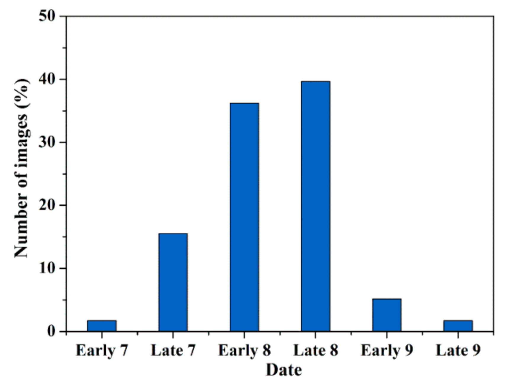
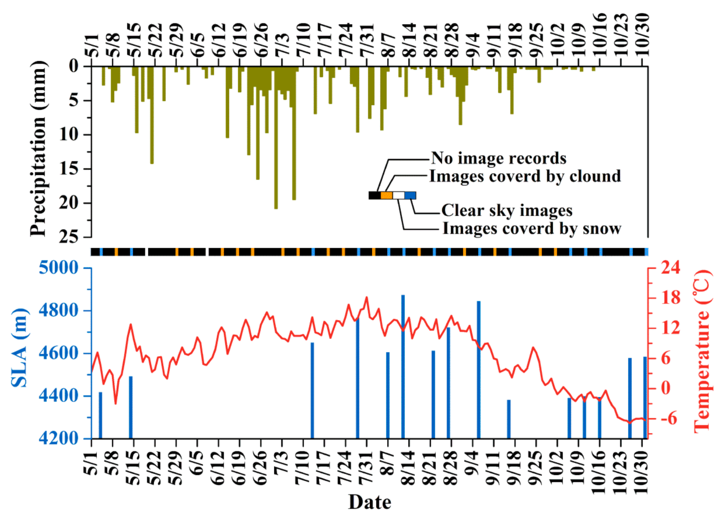
Landsat data have a high spatial resolution (30 m) and long time series, making them an ideal remote-sensing dataset for mapping glacier SLA. High Mountain Asia glaciers have a long melt season (generally the June–August timeframe), such that the highest SLA may occur on any day in either July or August (occasionally in early September). However, the data used in this study may not capture the highest SLA due to the large number of sensors and relatively low temporal resolution (8–16 days) of the Landsat satellites, which introduces a degree of uncertainty in the extracted SLA. Here we limit our data range for determining the glacier SLA to remote-sensing images that were acquired between 7 July and 15 September during the 1989–2019 period. Approximately 75% of the Landsat scenes that were analyzed for glacier SLA extraction were acquired in August (Figure 2).

Sentinel-2 data were used to evaluate the uncertainty in the Landsat-derived glacier SLA that arose from inconsistent Landsat data acquisition times since Sentinel-2 images possess a considerably higher spatiotemporal resolution. Sentinel 2A and 2B were launched in June 2015 and March 2017, respectively. Both satellites have a maximum spatial resolution of 10 m, and a temporal resolution to 5 days is achieved when Sentinel 2A and 2B data are analyzed together. We selected Sentinel-2 data that spanned the May 1–October 31, 2018 period for our analysis. Furthermore, the temporal proximity of the Sentinel-2 data to the Landsat data provides the opportunity to construct a long-term time series of glacier SLA from these two datasets.

Moderate Resolution Imaging Spectroradiometer (MODIS) data, which possess a high temporal resolution, were used to interpolate the glacier SLA where it was not extracted from the Landsat scenes. We preprocessed the MOD10A data to extract the glacier SLA [30], and then used Landsat data as the “true values” to verify the MODIS-derived glacier SLA, and obtain the annual snowline positions. We used the Shuttle Radar Topography Mission (SRTM) digital elevation model (DEM) (http://earthexplorer.usgs.gov/) to determine the snowline position on each analyzed glacier; the horizontal and vertical accuracies of the DEM are $\pm 20\mathrm{m}$ and $\pm 16\mathrm{m}$, respectively.

The meteorological data were obtained from the China Meteorological Data Service Center (http://data.cma.cn/) and NOAA National Climatic Data Center (NCDC) (http://www.ncdc.noaa.gov/).

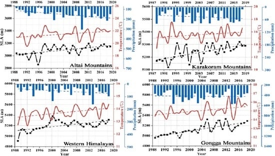
There are two main functions of the meteorological data in this study. The first is to evaluate the Landsat-derived SLA uncertainty using Sentinel 2 data. Temperature and precipitation data were also acquired from Tuole weather station, which is near Qiyi Glacier in the Qilian Mountains. The second function is to discuss the effects of temperature and precipitation on glacier SLA across High Mountain Asia. We acquired data from the nearest meteorological stations to the analyzed glacier areas during the 1998–2019 period; detailed information on the nearest meteorological stations in our study area is provided in

Table 2. Information on the nearest meteorological stations to the analyzed glacier areas.

Station ID	Name	Latitude	Longitude	Elevation (m)	Study Area
52633	Tuole	38°48′	98°25′	3368	Qiyi Glacier
51053	Haba River	48°03′	86°24′	533	Altai Mountains
51804	Tashkurgan	37°27′	75°08′	3090	Karakoram Mountains
55437	Purang	30°17′	81°15′	3900	Western Himalayas
56374	Kangding	30°1.8′	101°34′	2616	Gongga Mountains

. The analyzed glacier regions, with the exception of the Altai Mountains, mainly experience summer accumulation and melt, such that the average summer (June–August) temperature and precipitation were mainly collected for the analysis. We acquired summer precipitation and cold season (September–May) precipitation for the Altai Mountains since this region mainly experiences summer melt and cold season accumulation.

3.2. Methods

Data processing methods included data screening, pre-processing and SLA determination. Data screening mainly followed three criteria or principles: Landsat TM/ETM+/LC 8 images with (1) little cloud cover, (2) no recent snowfall on the glaciers, and (3) at the end of the summer melt season (July–August) were preferentially selected to enhance the probability of extracting the highest snowline or minimum snow cover. Image pre-processing included radiometric calibration, registration, atmospheric correction, and narrow-band to broadband albedo conversion. The subsequent delineation of the SLA was based on the registered DEM.

Radiation calibration is the process of converting a digital number (DN) to a corresponding radiation. The radiation of Landsat Level 1 product was calculated using the following equation:

L_λ = M_L × Q_cal + A_L

(1)

where L_λ is TOA spectral radiance [W (m⁻²·sr⁻¹·μm⁻¹)], M_L is band-specific gain from the metadata; Q_cal is quantized and calibrated standard product pixel values; and A_L is band-specific bias from the metadata.

Image registration is the process of matching and superposing two or more images acquired at different times, by different sensors (imaging devices) or under different conditions (i.e., weather, illumination, camera position and angle). In this study, Landsat image (ID: LT514402619980826, mean cloud cover: 4.57%) was taken as the base image to calibrate other Landsat images. The registered Landsat data was used as a base image to register the DEM data. This study utilized the ENVI software’s automatic accurate registration function, which makes the root mean square error (RMSE) of the ground control points less than 1, and performs quadratic polynomial correction to ensure registration accuracy and eventually obtains images with high registration quality.

Atmospheric correction can been used to reduce or eliminate the effect of atmospheric water vapor on the sensor, and can further calculate the narrowband albedo of the image. The FLAASH (Fast Line-of-sight Atmospheric Analysis of Spectral Hypercubes) module based on Modtran 4+ radiation transfer code was adopted in this study. This model can quickly perform atmospheric corrections of multispectral, hyperspectral data and aerial images, which could effectively eliminate the influence of atmosphere and light on the reflection of objects. The equation can be written as:

L = A × ρ/(1 − ρ_e × S) + B × ρ_e/(1 − ρ_e × S) + L_a

(2)

where L is the surface radiance [W (m⁻²·sr⁻¹·μm⁻¹)]; ρ is the pixel surface reflectance; ρ_e is the mean surface reflectance of the pixel and its surrounding regions; S is the spherical albedo of the atmosphere; L_a is the backscattering radiation of the atmosphere; and A, B is the coefficient which is related to the atmospheric and geometric conditions, but not to the underlying surface.

Our study determined the boundary between snow and bare ice based on the difference of their albedo. However, the albedo has not been directly obtained from satellites observations. Signals received by satellite sensors originate from radiances constitute radiation from a particular direction in narrowband at the top of the atmosphere. These signals must be converted to surface albedo. Based on near-surface and aircraft measurements, Greuell [31] established a narrowband-to-broadband albedo conversion model for glacier ice and snow, and it has a residual standard deviation of 0.011 for Landsat images. The equation is as follows:

α = 0.539 × ρ_i + 0.166 × ρ_j × (1 + ρ_j)

(3)

where α is the albedo; ρ is the narrowband albedo; i and j represent the specific band. For Landsat MSS, i and j represent the 1st and 3rd bands, respectively. For Landsat TM/ETM+, I and j represent the 2nd and 4th bands, respectively, because Landsat OLI has been changed in the band setting (a band is added in the visible band), and i and j represent the 3rd and 5th bands, respectively.

In order to calculate broadband albedo, the downloaded level-1C Sentinel 2 data need to conduct atmospheric correction. We will convert top-of-atmosphere reflectance of Level 1C Sentinel 2 data to surface reflectance data using the Sen2cor software. Sen2cor can be found on http://step.esa.int/main/third-party-plugins-2/sen2cor/. The atmospherically corrected Sentinel 2 data (Level 2A) were resembled using SNAP software and then converted to ENVI format for output. A narrow-to-broadband conversion was then performed through ENVI software to obtain the broadband albedo [32,33]. Snow line locations were determined based on the difference of albedo between the ice and snow. The snow line locations were extracted in the same way as the Landat data. In this case, the broadband albedo is obtained by the following equation,

A = 0.356ρ₂ + 0.130ρ₄ + 0.373ρ₈ + 0.085ρ₁₁ + 0.072ρ₁₂ − 0.0018

(4)

where α is the albedo; ρ is the narrowband albedo; 2, 4, 8, 11, and 12 represent the specific band of Sentinel 2.

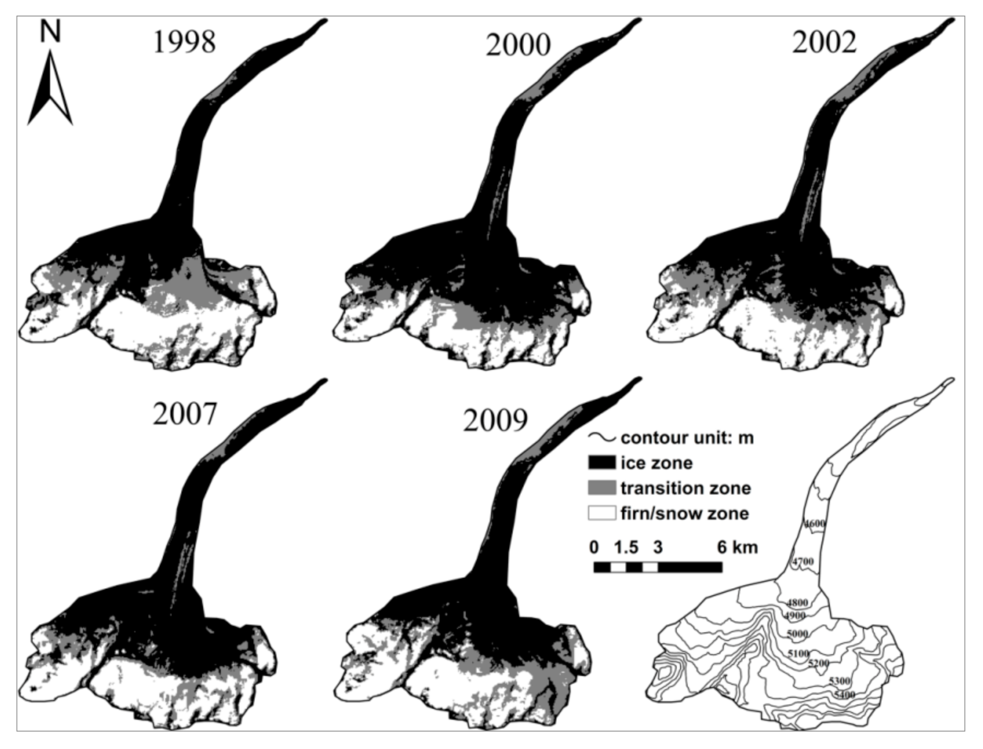
Based on the registered DEM data, its contour layer was extracted and overlaid with the broadband albedo image, and then the glacier surface was classified according to the difference between snow and bare ice albedo by ArcGIS software. If there was no transition zone between snow and bare ice, the boundary between snow and bare ice was defined as a snowline; if a transition zone existed, the boundary between snow and the transition zone was defined as a snowline. The SLA was then determined by the DEM contour layer by linking the lower edges of snowlines. It is possible that a snowline crosses several contours and does not coincide with a contour; in this case, the mean contour near the snowline was considered as the SLA [15,19] (Figure 3).

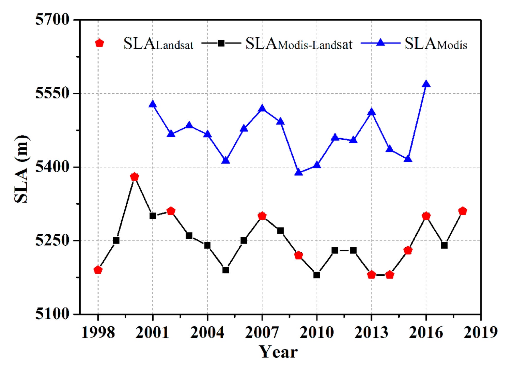
There are fewer available Landsat scenes for assessing the glacier SLA uncertainty over different dates in a given period due to the temporal resolution of the Landsat images and the impacts of clouds and new snowfall. We therefore combined the Sentinel-2 data, which possess a high temporal resolution (five days when using the data from 2A and 2B). Similarly, the Landsat temporal resolution, cloud cover, fresh snowfall, and stripe of the Landsat ETM data, all of which may result in missing data, could affect the glacier SLA time series reconstruction and analysis of glacier SLA variability over time. In particular, the glacier SLA in a given single year may determine the linear trend of the entire SLA, making it critical to have a complete SLA time series. MODIS data have a high temporal resolution (1 day) and long time series (data acquisition since 2000), but they possess a low spatial resolution (≤500 m); we therefore used the Landsat-derived SLAs as the “true values” to correct the MODIS-derived SLAs and further interpolate the Landsat-derived SLA time series (Figure 4).

4. Results and Discussions

4.1. Glacier SLA Accuracy Evaluation

Glacier SLA can reflect glacier changes, and is therefore a sensitive indicator of climate changes; these changes can be inferred from the degree of SLA variability. Furthermore, we can also estimate the glacier equilibrium line altitude (ELA), as well as the glacier mass balance, water volume, and runoff based on the SLA, highlighting the need to ensure the accuracy of the extracted SLA data. The glacier SLA accuracy is primarily affected by the data source (temporal and spatial resolution of the satellite imagery, and length of the data time series, if temporal glacier SLA changes are investigated). Cloud cover (especially in the southeastern region of the Tibetan Plateau), fresh snowfall, Landsat ETM data strips, and different extraction methods will likely affect the data accuracy. Furthermore, the precision of the DEM also determines the SLA accuracy since the DEM must be analyzed to obtain the glacier SLA. The accuracy of the extracted glacier SLA can generally be improved if the spatial resolution of the image is high. However, each data type has its own advantages and disadvantages when analyzing spatiotemporal SLA variability, such that joint analysis of multiple remote-sensing datasets can be considered.

We primarily selected images from the mid/late July–early September timeframe because the glacier SLA at the end of the ablation period should be the maximum SLA for a given year, which means that this SLA can represent the ELA. This image selection process also allowed us to evaluate and reduce the impact of image spatial resolution on glacier SLA. The ablation period mainly occurs in the June–August timeframe, although the highest SLA may be observed in early September if either warmer temperatures persist or there is little/no new precipitation. Approximately 90% of the analyzed Landsat images were acquired in the late July–August timeframe, with 75% acquired in August and 15% acquired in late July (Figure 2).

Sentinel-2 images (1 May–31 October 2018 timeframe) were also used to further evaluate the influence of the temporal resolution of the sensor on glacier SLA (Figure 5). The relationship between glacier SLA and temperature/precipitation during the ablation season was analyzed using the Sentinel-2 images, and temperature and precipitation observations from Tuole weather station, which is near Qiyi Glacier (Figure 5). We extracted the glacier SLA from 15 images during the ablation season due to the influences of new snowfall, cloud cover, and the temporal resolution of the satellite images. The glacier SLA was above 4600 m from July 28 to September 6, with a maximum SLA of 4873 m observed on August 12. The results indicated that the average variability from the highest SLA (August 12) during the late July–August timeframe was 132 m, with minimum and maximum variations of 29 and 268 m, respectively. These Sentinel-2-derived glacier SLA data suggest that our analysis of the Landsat scenes that were mainly acquired in August to extract glacier SLA could extract the highest glacier SLA. A comparison and analysis of our extracted glacier SLA positions with temperature and precipitation data revealed that the extracted SLAs from the late July–early September timeframe were high due to higher temperatures and less precipitation during this period. The highest SLA does not appear around July 31, when the temperature is highest, because there is more precipitation at the end of July. The highest SLA, which was acquired on August 12, was due to relatively high temperatures and less precipitation in the middle of August. Our correlation coefficient statistics indicate that glacier SLA is positively correlated with temperature (r = 0.56), which suggests that glacier SLA is mainly influenced by temperature. Temperature, precipitation, and SLA all show downward linear trends, which also indicates that temperature is the main factor influencing the observed glacier SLA variations.

We set a cloud cover threshold during the image filtering process, and then manually selected the appropriate images to avoid the influence of cloud cover on glacier SLA extraction. However, this resulted in the inability to obtain the SLA across some glaciers in a given year, which we express as “NA” in

Table 3. SLAs for the 12 analyzed glaciers across the Altai Mountains during the 1989–2019 period.

Year	SLA (m)
	A1	A2	A3	A4	A5	A6	A7	A8	A9	A10	A11	A12
1989	2880	2930	3270	3000	2950	2880	3210	3320	3080	3080	2900	2990
1993	2840	2860	NA	2910	2820	2760	3190	3070	2920	3030	2850	3040
1996	2600	2940	2980	2840	2730	2770	3210	3020	2820	2970	2740	2700
1998	3040	3120	3150	3210	2940	3110	3290	3440	3310	3350	3000	3300
2000	2750	3120	3140	3110	2970	2970	3100	3320	3200	3260	2990	3240
2001	NA	NA	3190	3090	3010	NA	3240	3440	3190	3260	2980	3180
2004	3030	3110	3160	NA	NA	3040	3310	3430	3250	NA	2970	3230
2006	2750	3050	3100	2950	2960	2880	3040	3300	3180	3240	2900	3170
2007	3060	NA	NA	3060	3000	NA	3230	3480	3200	3290	2970	3170
2008	3020	3140	3140	3120	2990	2850	3090	3210	3080	3220	3000	3240
2009	2740	3030	3090	2960	2920	2820	3070	3390	3090	3120	2900	3036
2010	3070	3070	3250	3070	2960	2920	3200	3470	3070	3190	2980	3030
2012	3100	3160	3180	3270	2960	2920	3290	3380	3300	3410	3130	3250
2013	2730	3010	NA	3090	3140	NA	3210	3380	3140	3180	2910	3050
2015	2960	3110	3170	3030	2930	2920	3220	3540	3220	3280	2960	3090
2016	3020	3140	3180	3100	3010	2960	3270	3480	3280	3330	2980	3280
2017	3090	3130	3200	3120	3030	2940	3230	3470	3330	3310	3130	3240
2019	2980	3110	NA	3050	2970	2930	3260	3460	3280	3330	2990	3270

. We also manually filtered the images with no fresh snowfall to avoid the effects of new snowfall. We note that there were stripes in the Landsat ETM data after 2003; these stripes were removed by applying nearest-neighbor interpolation to estimate the pixel values of the area covered by land. We extracted the snow line based on the albedo difference between the ice and snow, and set a threshold to segment the ice surface, with the boundary between the snow and ice marking the position of the snow line. The boundary between the snow and transition zone was treated as the location of the snow line if a transition zone was present. The albedo was obtained via our inversion approach, which is outlined in Section 3. Previous studies have shown that the absolute error between the albedo retrieved from Qiyi Glacier and the measured albedo is within 0.05 [34]. A DEM with a higher spatial resolution can be used to improve the accuracy of the glacier SLA; therefore, we used a SRTM DEM that possessed a 30 m spatial resolution and ~16 m linear vertical absolute height error to ensure the high accuracy of the extracted glacier SLAs.

4.2. Glacier SLA across the Altai Mountains

The glacier SLA across the Altai Mountains is presented in Table 3. We were unable to determine the SLA of some glaciers in a given year due to occasional cloud cover. The lowest and highest SLAs in the time series were 2600 m at A1 Glacier in 1996 and 3540 m at A8 Glacier in 2015, respectively, with 940 m of variability among the 12 analyzed glaciers. The SLA changes for the individual glaciers across Altai Mountains during the 1989–2019 period are shown in Figure 6. All of the glacier SLAs exhibit an upward trend. The SLA change of an individual glacier was in the 31–302 m range during the study period, with most of the analyzed glaciers exhibiting SLA changes in the 100–300 m range; A8 Glacier possessed the largest change (Figure 6a). Three glaciers (A3, A6, and A7) possessed a relatively stable SLAs, with an average increase of 42 m. The largest SLA variability during the study period was observed along A1 Glacier (SD = 156 m), whereas A3 Glacier possessed the smallest SLA variability (SD = 71 m; Figure 6b). The mean SLA of A8 Glacier was the highest among the analyzed glaciers across the Altai Mountains (3370 ± 142 m), and A6 Glacier possessed the lowest mean SLA at 2910 ± 92 m. The reason for the large SLA difference or variability among the 12 glaciers in a given year may be related to spatial differences in precipitation, temperature, and/or topography (such as aspect and slope).

The mean glacier SLA variability at the end of the melt season (generally August) across the Altai Mountains during the 1989–2019 period is shown in Figure 7. The mean glacier SLA generally increased over time, which indicates that the glaciers were in a state of ablation throughout the 1989–2019 period. The SLAs ranged from 2860 ± 169 m in 1996 to 3260 ± 152 m in 2012, with a maximum variability of 721 m. Furthermore, linear regression analysis revealed that the mean glacier SLA across the Altai Mountains declined by 151 m during the 1989–2019 period.

Meteorological data from the Haba River weather station were used to determine the effects of temperature and precipitation on glacier SLA across the Altai Mountains. The general temperature and precipitation trends should be similar in a relatively small region, such as the weather station and nearby glaciers, even though regional variations in the meteorological conditions exist. We calculated the total precipitation for the September–May timeframe and summer mean temperature for the June–August timeframe since these glaciers generally experienced accumulation during the cold season and strong ablation during the summer (Figure 7). The cold season precipitation and summer mean temperature both increased during our analysis period, suggesting that increased summer ablation might be the key reason for the increased SLA. The mean glacier SLA observations across the Altai Mountains generally exhibited a significant positive correlation with temperature (Figure 7). We calculated the correlation coefficients between mean SLA and summer mean temperature (r = 0.55; 95% confidence level) and cold season precipitation (r = 0.38), with the summer mean temperature being the primary factor influencing glacier SLA across the Altai Mountains. The linear trends in summer mean temperature and mean SLA further suggest that temperature exerts the primary influence on the glacier SLA changes across the Altai Mountains.

4.3. Glacier SLA across the Karakoram Mountains

The glacier SLA across the Karakoram Mountains is shown in

Table 4. SLA of the nine analyzed glaciers across the Karakoram Mountains during the 1989–2019 period.

Year	Snowline Altitude (m)
	K1	K2	K3	K4	K5	K6	K7	K8	K9
1991	5210	5190	5070	5200	5500	5060	5080	5110	5150
1993	5110	4900	4950	5090	5370	5010	5190	5160	5330
1994	5130	5130	5050	4980	5460	5310	5220	5120	5180
1996	5030	5120	NA	5520	5540	5170	5240	5400	5440
1997	5190	5100	5070	5130	5480	5210	5200	5230	5420
1999	5050	NA	NA	NA	NA	NA	5250	5420	5490
2000	5060	5150	4920	5220	5420	5060	NA	NA	NA
2001	5070	5170	4970	5350	5470	5290	5230	5270	5330
2002	5040	5200	4800	5300	5640	5270	NA	5300	5480
2004	5030	5140	4850	5160	5510	5190	5200	5110	NA
2005	5050	5150	4930	5290	5490	5280	5230	5340	5340
2006	5060	5200	5040	5370	5550	5390	5260	5430	5490
2007	5050	5190	NA	5290	NA	5300	NA	NA	5410
2009	5040	5150	4800	5210	5440	5250	5230	5490	5510
2010	5040	5140	4710	5230	5470	5260	5260	5530	5390
2011	5060	5160	NA	5110	5520	5240	5240	5430	5540
2013	NA	5160	4880	5310	5510	5300	5260	5660	5490
2014	5190	5140	5090	5180	5490	5210	5190	5440	5320
2015	5030	5160	5100	5190	5560	5240	5140	5600	5320
2017	5200	5160	NA	5220	5580	5300	5230	5380	5470
2018	5210	5170	5100	5210	5610	5260	5260	5380	5420
2019	5200	5180	5090	5210	5580	5260	5260	5580	5290

. It varied by 950 m, ranging from 4710 m at K3 Glacier in 2010 to 5660 m at K8 Glacier in 2013. The individual mean glacier SLA changes ranged from 22 to 412 m during the study period (Figure 8a), with K1, K3, and K4 glaciers exhibiting slight SLA changes (<50 m increase), and K8 Glacier exhibiting a 412 m increase over the past 30 years. Four glacier SLAs exhibited increases of >100 m. K8 Glacier exhibited the largest SLA variability (SD = 164 m; Figure 8b), whereas K7 Glacier possessed a relatively stable SLA (SD = 46 m) during the 1989–2019 period. K5 Glacier possessed the highest mean SLA at 5510 ± 66 m, and K3 Glacier possessed the lowest mean SLA at 4970 ± 124 m.

The mean SLA across the Karakoram Mountains at the end of the melt season (generally August) during the 1989–2019 period is shown in Figure 9. There is an obvious increase in mean glacier SLA over time, with a maximum increase from 5120 ± 159 m in 1993 to 5320 ± 240 m in 2013, which indicates that these glaciers were in a state of mass loss during the analysis period. Linear regression analysis of the SLA time series revealed a 123-m increase in mean SLA across this region during the 1989–2019 period.

We calculated the precipitation and mean temperature from the June–August (summer) observations at Tashkurgan weather station since the Karakoram Mountains experience both summer accumulation and ablation (Figure 9). The summer precipitation and temperature in the Karakoram Mountains both exhibited increasing trends over the study period. Temperature may therefore contribute to the increase in glacier SLA. The mean SLA across the Karakoram Mountains during the 1989–2019 period exhibited a strong positive correlation with summer mean temperature. The lowest SLA was observed in 1993, followed by an SLA of 5140 ± 171 m in 2000. The lowest summer mean temperature occurred in 1989. However, the difference in SLA between 2000 and 2004 was only 20 m, which was within the uncertainties of the SLA derivation. The highest glacier SLA was observed in 2013, when the mean summer mean temperature was 17.23 °C and there was relatively little precipitation (~50 mm). The correlation coefficients between mean glacier SLA and the summer mean temperature and summer precipitation in the Karakoram Mountains were 0.41 and 0.03, respectively. The mean SLA across the Karakoram Mountains during the 1989–2019 period exhibited an obvious positive correlation with summer mean temperature. The linear trends in summer mean temperature and mean SLA further suggest that temperature is the primary factor influencing the observed glacier SLA changes across the Karakoram Mountains.

4.4. Glacier SLA across the Western Himalayas

The glacier SLA across the Western Himalayas is presented in

Table 5. SLAs of the 12 analyzed glaciers across the Western Himalayas during the 1989–2018 period.

Year	Snowline Altitude (m)
	H1	H2	H3	H4	H5	H6	H7	H8	H9	H10	H11	H12
1989	4650	4720	4850	5070	4980	5090	5100	4810	5010	4920	5130	4560
1991	NA	4890	5250	523	5160	5200	5250	NA	5060	5190	5080	4900
1992	4890	4880	5160	5130	5040	5220	5310	NA	5030	5060	4950	4840
1993	5150	4790	5180	5160	5340	5190	5250	4830	4990	4920	5000	4860
1994	4970	4890	5220	5250	5360	5300	5230	5160	5090	5020	5040	4880
1998	5290	4890	5230	5270	5310	5320	5290	5190	5170	5180	5300	4870
2000	5500	4920	5500	5430	5460	5460	5420	5290	5370	5520	5440	5290
2002	5310	4970	5530	5310	5420	5370	5340	5240	5310	5300	5330	5330
2004	5310	4960	5460	5380	5420	5460	5340	5220	5150	5280	5380	4970
2007	5290	5100	5500	5290	5370	5410	5330	5270	5290	5230	5360	5130
2009	5100	5010	5410	5250	5370	5240	5240	5210	5110	5190	5260	4940
2011	5200	5400	5270	5240	5240	5240	5230	5170	5090	5160	5260	4860
2013	5120	4950	5330	5250	5380	5260	5040	5200	5060	5210	5140	NA
2014	5230	4930	5250	5260	NA	5250	5380	NA	5180	5210	5210	4900
2015	5270	4980	5410	5380	5110	5300	5290	NA	5350	5220	5310	4890
2016	5210	5080	5440	5300	5400	5350	5340	5250	5220	5300	5370	5300
2018	5410	4940	5480	5390	5430	5460	5350	5260	5290	5370	5390	5000

. The SLA varied by 970 m, ranging from 4560 m at H12 Glacier in 1989 to 5530 m at H3 Glacier in 2002. The SLA changes for individual glaciers during the 1989–2018 period are shown in Figure 10. Each analyzed glacier exhibited an increasing SLA trend in the Western Himalayas during the 1989–2018 period (Figure 10a), with glacier SLA increases of 60–357 m. H7 and H1 glaciers exhibited the smallest and largest increases, respectively, with most glaciers exhibiting SLA increases in the 100–300 m range. H1 Glacier also exhibited the largest SLA variability (SD = 207 m; Figure 10b), whereas H4 Glacier possessed a relatively stable SLA during the 1989–2018 period (SD = 94 m). H3 Glacier exhibited the highest mean SLA at 5320 ± 173 m, and H2 Glacier exhibited the lowest mean SLA at 4960 ± 173 m.

The mean SLA across the Western Himalayas at the end of the melt season (generally August) during the 1989–2018 period is shown in Figure 11. The mean SLA exhibited a gradual increase over time, which indicates that these glaciers were in a state of mass loss during the analysis period. The maximum and minimum SLAs were 4910 ± 190 m in 1989 and 5380 ± 164 m in 2000, respectively. Linear regression analysis of the SLA time series revealed that the mean SLA increased from 5110 m to 5300 m across the Western Himalayas during the 1989–2018 period.

We calculated both the precipitation and mean temperature from the June–August (summer) observations at the Purang weather station since the Western Himalayas experience both summer accumulation and ablation (Figure 11). The mean summer mean temperature and precipitation both exhibited increasing trends in the Western Himalayas during the analysis period, suggesting that temperature was the main cause of the increasing SLA across the Western Himalayas during the 1989–2018 period. The mean temperature was above 12.5 °C for most of the time series, ranging from 12.6 °C in 1992 to 14.4 °C in 2006.

The mean glacier SLA across the Western Himalayas during the 1989–2018 period exhibited a positive correlation with summer mean temperature (r = 0.54), which suggests that the summer mean temperature across the Western Himalayas is the main factor influencing glacier SLA. The observed relationship between glacier SLA and temperature further supports the influence of summer mean temperature on glacier SLA across the Western Himalayas.

4.5. Glacier SLA across the Gongga Mountains

The SLA for each of these glaciers is shown in

Table 6. SLA of the five analyzed glaciers across the Gongga Mountains during the 1989–2019 period.

Year	Snowline Altitude (m)
	G1	G2	G3	G4	G5
1989	4970	4840	5000	4970	5020
1990	4980	4870	5040	5060	4960
1994	5160	4970	5060	4990	5030
1995	5120	5020	5080	5080	5070
1997	5030	4830	4980	NA	4980
1998	5230	4810	5220	NA	5000
1999	5160	5040	5110	5150	4980
2000	5180	5060	5180	5020	5050
2003	5090	5070	5100	5010	5010
2006	5250	5350	5370	NA	NA
2007	5150	5150	5110	5000	5040
2009	5240	5290	5300	5310	5100
2010	5310	5310	5430	5320	5120
2011	5110	5120	5030	5300	5090
2012	5290	NA	5440	NA	5250
2013	5180	5370	5150	NA	5040
2014	5130	5060	5070	NA	NA
2016	5250	4980	5360	5320	5070
2019	5320	5240	5310	5350	5240

. The mean SLA of each analyzed glacier exhibited a remarkable increasing trend, ranging from 188 m at G5 Glacier to 405 m at G2 Glacier (Figure 12a), with four glaciers exhibiting an increase in SLA of more than 300 m during the 30-year analysis period. The SLA varied by 630 m across the Gongga Mountains, ranging from 4810 m at G2 Glacier in 1998 to 5440 m at G3 Glacier in 2012. G2 Glacier exhibited the largest SLA variability (SD = 180 m; Figure 12b), whereas G5 Glacier exhibited the smallest SLA variability (SD = 82 m). G3 Glacier exhibited the highest mean SLA at 5180 ± 149 m, and G5 Glacier exhibited the lowest mean SLA at 5060 ± 82 m.

The mean glacier SLA across the Gongga Mountains at the end of the melt season (generally August) during the 1989–2019 period is shown in Figure 13. The mean SLA generally increased over time, which indicates that these glaciers were in a state of mass loss during the 30-year analysis period. The mean SLA varied by 540 m, ranging from 4960 ± 70 m in 1989 to 5330 ± 100 m in 2012. Linear regression analysis revealed a mean SLA increase of 282 m across the Gongga Mountains during the 1989–2019 period.

Meteorological data from the Kangding weather station, which is the closest weather station to the Gongga Mountains, were analyzed to determine the effects of temperature and precipitation on glacier SLA. We calculated the summer (June–August) precipitation and mean temperature since the glaciers across the Gongga Mountains experience both accumulation and strong ablation during the summer months (Figure 13). Increasing trends are observed in both the summer mean temperature and precipitation values, suggesting that increasing temperatures may be accelerating ablation, resulting in the increasing SLAs across the Gongga Mountains during the 1989–2019 period. The mean SLA across the Gongga Mountains during the 1989–2019 period exhibited a positive correlation with summer mean temperature (r = 0.44), which indicates that the glacier SLA across the Gongga Mountains area was primarily influenced by temperature.

4.6. Glacier SLA for Different Orientations across the Westerlies and the Monsoon Control Zone

Due to spatial variation of entire mountains ranges and differences in the number of glaciers in various orientations, uncertainty exists in the discussion of SLA changes in different orientations. Therefore, we selected the SLA of different orientations of peaks where the glaciers are concentrated to analyze the influence of the windward slope of the westerlies and monsoon water vapor in the westerly wind belt. The Tian Shan and the Nyainqentanglha Mountains were selected to represent glaciers influenced by the westerlies and the monsoon, respectively. A total of 42 glaciers in the Tian Shan and 37 glaciers in the Nyainqentanglha Mountains were selected. The number of glaciers distributed in different orientations are listed in

Table 7. The number of glaciers in different orientations in the Tian Shan and the Nyainqentanglha Mountains.

Study Area	Number of Glaciers in Different Orientations
	N	E	S	W
Tian Shan	22	9	12	15
Nyainqentanglha Mountains	20	22	15	11

, and their mean SLA are calculated (Figure 14).

The mean SLA of the Tian Shan glaciers toward the east is higher than that toward the west because the Tian Shan climate is dominated by the westerlies. The glaciers facing west are located on the windward slope, where the airstream that comes from the western or northwestern direction is blocked, and precipitation is thus greater than in the east. This leads to lower SLA in the west of the glaciers compared to the east. At the same time, the mean SLA of the southward glaciers is higher than that of the northward glaciers. This is because the southern slope receives more solar radiation than the northern slope, as well as that the southern side is affected by the dry and hot climate of the Tarim Basin desert in summer. Furthermore, SLA differences between southward and northward glaciers are much greater than that of the eastward and westward glaciers, probably indicating that the effect of temperature on SLA is greater than the effect of precipitation on SLA.

The mean SLA of the southward glacier in the Nyainqentanglha Mountains is lower than that of the northward glacier. The selected glaciers are concentrated in the eastern segment of the Nyainqentanglha Mountains, where they converge with the Hengduan Mountains to form a trumpet-shaped terrain, its climate is mainly controlled by the Indian monsoon, and the southern slope of the mountain constitutes a barrier of the Indian monsoon moving north. The south slope is the windward slope with more precipitation than the northern slope (rain shadow zone), resulting in lower SLA of the southward glacier than that of the northward glaciers. The SLA of the eastward glaciers is higher than that of the westward glacier because the solar radiation on the eastern slope is higher than that of the western slope. The SLA differences between the eastward and westward glaciers are greater than those toward the south and north glaciers. This probably also indicates that temperature is also the main factor that affects the SLA of the Nyainqentanglha Mountains.

There was a sharp decrease in precipitation from the eastern and southeastern marginal mountains of the Tibetan Plateau to the west and northwest during the 1989–2019 period, whereas the maximum temperature occurred in the western region of the Tibetan Plateau. Regional hydrological conditions could therefore cause an east (southeast) to west (northwest) increase in glacier SLA, as shown in Figure 15, where the maximum glacier SLA occurred on the northern slopes of the Western Himalayas. The SLAs on the eastern side of the plateau were lower and exhibited an east-to-west longitudinal pattern of increasing glacier SLA. Glacier SLA generally increased with decreasing latitude from the Altai Mountains to the Karakoram Mountains; conversely, glacier SLA decreased with decreasing latitude across the Himalayan region. The glacier SLA across the Altai Mountains was mainly influenced by the westerly wind zone. The glacier scale to the east of the distribution center of the main glaciers formed by Friendship Peak and Kuitun Peak decreased with decreasing mountain height and annual precipitation, resulting in an increase in glacier SLA from 3100 m in the Burqin River Basin to 3800 m in the Ulungu River Basin. The glacier SLA across the Karakoram Mountains gradually increased from west to east, ranging from 5000 to 5800 m, with the western section being significantly influenced by the westerly flow zone. The Himalayan SLA ranged from 5800 m on the northern slope to 4700 m on the southern slope. The Himalayas block the northward flow of the Indian monsoon zone, leading to the northern slope and more northerly region being drier than the southern slope. The Himalayan SLA therefore exhibited an abnormal SLA distribution, with low glacier SLAs on the southern slope and high glacier SLAs on the northern slope. The glacier SLA across the Hengduan Mountains was in the 4900–5200 m range. The western part of the Hengduan Mountains is located in the water vapor transport zone of the southeast monsoon, with abundant precipitation causing the glacier SLAs to extend upglacier in a tongue shape, revealing a gradual increase in SLA from the outside to the inside of a given glacier. The glacier SLAs on the eastern side of the Hengduan Mountains exhibited a longitudinal SLA pattern, with an east-to-west increase in glacier SLA.

5. Conclusions

Glacier SLA is an indicator of glacier ELA, which is a key parameter for predicting climate behavior and change. We derived the glacier SLA across High Mountain Asia and analyzed the observed SLA changes, and their relationship to temperature and precipitation observations over the past ~30 years. The selected glaciers are largely located in regions where the climate is controlled by the westerlies and/or monsoons.

Our results demonstrate that summer mean temperature is the primary factor influencing the observed glacier SLA changes across High Mountain Asia, with precipitation also playing a major role in some regions.

The mean SLA across the Altai Mountains, Karakoram Mountains, Western Himalayas, and Gongga Mountains increased during the 1989–2019 period. The mean glacier SLA across the Altai Mountains ranged from 2860 ± 169 m to 3200 ± 152 m, and the mean glacier SLA across the Karakoram Mountains varied from 5120 ± 159 m in 1993 to 5320 ± 240 m in 2013, with the glaciers across both regions experiencing an average SLA increase of 123–151 m over the past 30 years. The mean glacier SLA across the Western Himalayas and Gongga Mountains increased by 190–282 m over the past 30 years, with the mean SLA across the Western Himalayas ranging from 4910 ± 190 m in 1989 to 5380 ± 164 m in 2000, and that across the Gongga Mountains increasing from 4960 ± 70 m to 5330 ± 100 m. The was a general increase in glacier SLA from the Altai Mountains to the Karakoram Mountains, with a decrease in glacier SLA with decreasing latitude across the Himalayas; the maximum SLA occurred near the northern slopes of the Western Himalayas. The glacier SLAs were in the 3100–3800, 5000–5800, 5800–4700, and 4900–5200 m ranges across the Altai Mountains, Karakoram Mountains, Western Himalayas, and Hengduan Mountains, respectively. Correlation analyses between glacier SLA and temperature/precipitation suggested that the mean glacier SLAs in the study areas were mainly influenced by temperature. Furthermore, the glacier SLA in the westerlies (Tian Shan) and monsoon control zones (Nyainqentanglha Mountains) are affected by both temperature and precipitation. However, temperature appears to generally play a more important role than precipitation.

The accuracy in mapping glacier SLA depends on the quality of the remote-sensing image, precision of the resultant DEM, and extraction method. Since optical remote sensing is greatly influenced by cloud cover, which is especially prevalent in the southeastern Tibetan imagery, future work should include further improvements in mapping glacier SLA across these poorly imaged regions, and then extending this methodology to the entire High Mountain Asia region to better capture regional climate change, and provide more accurate constraints for mass balance studies and for snowmelt runoff and hydrological models.

References

1. Immerzeel, W.W.; Beek, L.P.H.V.; Bierkens, M.F.P. Climate Change Will Affect the Asian Water Towers. Science 2010, 328, 1382–1385. [Google Scholar] [CrossRef] [PubMed]
2. Chen, X.Y.; Zhang, X.B.; Church, J.A.; Watson, C.S.; King, M.A.; Monselesan, D.; Legresy, B.; Harig, C. The Increasing Rate of Global Mean Sea-Level Rise during 1993–2014. Nat. Clim. Chang. 2017, 7, 492–495. [Google Scholar] [CrossRef]
3. Wang, W.C.; Xiang, Y.; Gao, Y.; Lu, A.X.; Yao, T.D. Rapid Expansion of Glacial Lakes Caused by Climate and Glacier Retreat in The Central Himalayas. Hydrol. Process. 2015, 29, 859–874. [Google Scholar] [CrossRef]
4. Gardner, A.S.; Moholdt, G.; Cogley, J.G.; Wouters, B.; Arendt, A.A.; Wahr, J.; Berthier, E.; Hock, R.; Pfeffer, W.T.; Kaser, G.; et al. A Reconciled Estimate of Glacier Contributions to Sea Level Rise: 2003 to 2009. Science 2013, 340, 852–857. [Google Scholar] [CrossRef] [PubMed] [Green Version]
5. Brahmbhatt, R.M.; Bahuguna, I.; Rathore, B.P.; Kulkarni, A.V.; Shah, R.D.; Nainwal, H.C.; Prof, A. Variation of Snowline and Mass Balance of Glaciers of Warwan and Bhut Basins of Western Himalaya Using Remote Sensing Technique. J. Indian Soc. Remote 2012, 40, 629–637. [Google Scholar] [CrossRef]
6. Rabatel, A.; Dedieu, J.P.; Vincent, C. Spatio-Temporal Changes in Glacier-Wide Mass Balance Quantified by Optical Remote Sensing on 30 Glaciers in the French Alps for the Period 1983–2014. J. Glaciol. 2016, 62, 1153–1166. [Google Scholar] [CrossRef] [Green Version]
7. Zhang, Z.M.; Jiang, L.M.; Liu, L.; Sun, Y.F.; Wang, H.S. Annual Glacier-Wide Mass Balance (2000–2016) of the Interior Tibetan Plateau Reconstructed from MODIS Albedo Products. Remote Sens. 2018, 10, 1031. [Google Scholar] [CrossRef] [Green Version]
8. Paterson, W.S.B. The Physics of Glaciers, 3rd ed.; Elsevier Science: Oxford, UK, 1994. [Google Scholar]
9. Rabatel, A.; Bermejo, A.; Loarte, E.; Soruco, A.; Gomez, J.; Leonardini, G.; Vincent, C.; Sicart, J.E. Can the Snowline Be Used as an Indicator of the Equilibrium Line and Mass Balance for Glaciers in the Outer Tropics? J. Glaciol. 2012, 58, 1327–1336. [Google Scholar] [CrossRef] [Green Version]
10. Mernild, S.H.; Pelto, M.; Malmros, J.K.; Yde, J.C.; Knudsen, N.T.; Hanna, E. Identification of Snow Ablation Rate, ELA, AAR and Net Mass Balance Using Transient Snowline Variations on two Arctic Glaciers. J. Glaciol. 2013, 59, 649–659. [Google Scholar] [CrossRef] [Green Version]
11. Rabatel, A.; Dedieu, J.P.; Vincent, C. Using Remote-Sensing Data to Determine Equilibrium-Line Altitude and Mass-Balance Time Series: Validation on Three French Glaciers, 1994–2002. J. Glaciol. 2005, 51, 539–546. [Google Scholar] [CrossRef] [Green Version]
12. Rees, W.G. Remote Sensing of Snow and Ice, 1st ed.; CRC Press: Boca Raton, FL, USA, 2005. [Google Scholar]
13. De Angelis, H.; Rau, F.; Skvarca, P. Snow Zonation on Hielo Patagónico Sur, Southern Patagonia, Derived from Landsat 5 TM Data. Glob. Planet. Chang. 2007, 59, 149–158. [Google Scholar] [CrossRef]
14. Hu, Z.Y.; Dietz, A.; Kuenzer, C. The Potential of Retrieving Snow Line Dynamics from Landsat during the End of the Ablation Seasons between 1982 and 2017 in European Mountains. Int. J. Appl. Earth Obs. Geoinf. 2019, 78, 138–148. [Google Scholar] [CrossRef]
15. McFadden, E.M.; Ramage, J.M.; Rodbell, D. Landsat TM and ETM+ Derived Snowline Altitudes in the Cordillera Huayhuash and Cordillera Raura, Peru, 1986–2005. Cryosphere 2011, 5, 419–430. [Google Scholar] [CrossRef] [Green Version]
16. Guo, Z.M.; Wang, N.L.; Wu, H.B.; Wu, Y.W.; Wu, X.J.; Li, Q.L. Variations in Firn Line Altitude and Firn Zone Area on Qiyi Glacier, Qilian Mountains, over the Period of 1990 to 2011. Arct. Antarct. Alp. Res. 2015, 47, 293–300. [Google Scholar] [CrossRef] [Green Version]
17. Pelto, M. Utility of Late Summer Transient Snowline Migration Rate on Taku Glacier, Alaska. Cryosphere 2011, 5, 1127–1133. [Google Scholar] [CrossRef]
18. Zhang, Q.B.; Kang, S.C. Glacier Snowline Altitude Variations in the Pamirs, Tajikistan, 1998–2013: Insights from Remote Sensing Images. Remote Sens. Lett. 2017, 8, 1220–1229. [Google Scholar] [CrossRef]
19. Kaur, R.; Saikumar, D.; Kulkarni, A.V.; Chaudhary, B.S. Variations in Snowcover and Snowline Altitude in Baspa Basin. Curr. Sci. India 2009, 96, 1255–1258. [Google Scholar]
20. Guo, Z.M.; Wang, N.L.; Kehrwald, N.M.; Mao, R.J.; Wu, H.B.; Wu, Y.W.; Jiang, X. Temporal and Spatial Changes in Western Himalayan Firn Line Altitudes from 1998 to 2009. Glob. Planet. Chang. 2014, 118, 97–105. [Google Scholar] [CrossRef]
21. Chen, M.D. Spatio-temporal Change Dynamic of Snowline on Tibetan Plateau; Lanzhou University: Lanzhou, China, 2014. [Google Scholar]
22. Shi, J.; Bai, S.; Gao, J.; Gu, H. Spatial and Temporal Variation of Snow Line and Its Relationships with Meteorological Factors in Tibet Plateau in Recent 10 Years. Desert Oasis Meteorol. 2015, 9, 7–13. [Google Scholar]
23. Tang, Z.; Wang, J.; Liang, J.; Li, C.; Wang, X. Monitoring of Snowline Altitude over the Tibetan Plateau Based on MODIS Data. Remote Sens. Technol. Appl. 2015, 30, 767–774. [Google Scholar]
24. Bao, W.J.; Liu, S.Y.; Wu, K.P.; Wang, R.J.; Jiang, Z.L. A Method for Extracting Snow Line Altitude Based on MODIS Snow Product. J. Glaciol. Geocryol. 2017, 39, 259–272. [Google Scholar]
25. Consortium, RGI. Randolph Glacier Inventory–A Dataset of Global Glacier Outlines: Version 5.0: Technical Report, Global Land Ice Measurements from Space, Boulder Colorado, the United States of America. 2015. Digital Media. Available online: www.glims.org/RGI (accessed on 15 December 2020).
26. Yao, T.; Thompson, L.; Yang, W.; Yu, W.; Gao, Y.; Guo, X.; Yang, X.; Duan, K.; Zhao, H.; Xu, B.; et al. Different Glacier Status with Atmospheric Circulations in Tibetan Plateau and Surroundings. Nat. Clim. Chang. 2012, 2, 663–667. [Google Scholar] [CrossRef]
27. Xie, Z.; Zhou, Z.; Li, Q.; Wang, S. Progress and Prospects of Mass Balance Characterist and Responding to Global Change of Glacier System in High Asia. Adv. Earth Sci. 2009, 24, 1065–1072. [Google Scholar]
28. Shih, Y.; Hsieh, T.; Cheng, P.H.; Li, C. Distribution, Features and Variations of Glaciers in China World Glacier Inventory; IAHS–AISH, Dorking, Eng.: International Association of Hydrological Sciences: Riederalp, Switzerland, 1980; Volume 126, pp. 111–116. [Google Scholar]
29. Lanzhou Institute of Glaciology and Cryopedology; Chinese Academy of Sciences. An Introduction to the Glaciers in China; Science Press: Beijing, China, 1988. [Google Scholar]
30. Tang, Z.; Wang, X.; Wang, J.; Wang, X.; Wei, J. Investigating Spatiotemporal Patterns of Snowline Altitude at the End of Melting Season in High Mountain Asia, Using Cloud-Free MODIS Snow Cover Product, 2001–2016. Cryosphere Discuss. 2019. Available online: https://tc.copernicus.org/preprints/tc-2019-139/ (accessed on 15 December 2020).
31. Greuell, W.; Reijmer, C.H.; Oerlemans, J. Narrowband-to-Broadband Albedo Conversion for Glacier Ice and Snow Based on Aircraft and Near-Surface Measurements. Remote Sens. Environ. 2002, 82, 48–63. [Google Scholar] [CrossRef]
32. Liang, S. Narrowband to Broadband Converions of Land Surface Albedo: I Algorithms. Remote Sens. Environ. 2000, 76, 213–238. [Google Scholar] [CrossRef]
33. Naegeli, K.; Damm, A.; Huss, M.; Wulf, H.; Schaepman, M.; Hoelzle, M. Cross-Comparison of Albedo Products for Glacier Surfaces Derived from Airborne and Satellite (Sentinel-2 and Landsat 8) Optical Data. Remote Sens. 2017, 9, 110. [Google Scholar] [CrossRef] [Green Version]
34. Mao, R.J.; Jiang, X.; Guo, Z.M.; Wu, H.B.; Wang, S. Study of the Inversion Precision of Albedo on the Qiyi Glacier in the Qilian Mountain Based on TM/ETM+ Image. J. Glaciol. Geocryol. 2013, 35, 301–309. [Google Scholar]
Figure 1. Location of the study area and primary wind circulation patterns. The black triangle represents the glaciers located in the Altai Mountains, the Karakoram Mountains, the Western Himalayas and the Gongga Mountains to identify the snowline altitude (SLA).
Remotesensing 13 00425 g001
Figure 2. Temporal distribution of the selected Landsat images to derive SLA.
Remotesensing 13 00425 g002
Figure 3. The distribution of bare ice and snow-covered areas based on appreciably different albedo on the Shamshar gang glacier in Western Himalayan in 1998, 2000, 2002, 2007, and 2009 [20].
Remotesensing 13 00425 g003
Figure 4. Landsat- and MODIS-derived SLA time series, with the Landsat-derived SLAs taken as the “true values” (example from the Western Himalayas presented). SLAModis, SLALandsat, and SLAModis-Landsat represent the MODIS-derived SLA, Landsat-derived SLA, and Landsat-derived SLA with MODIS interpolation, respectively.
Remotesensing 13 00425 g004
Figure 5. Glacier SLAs that were extracted from the Sentinel-2 images during the ablation season.
Remotesensing 13 00425 g005
Figure 6. (a) SLA changes and (b) mean SLA of the 12 analyzed glaciers across the Altai Mountains during the 1989–2019 period. The error bars in (b) represent one standard deviation from the mean.
Remotesensing 13 00425 g006
Figure 7. Cold season (September–May) precipitation (blue), summer mean temperature (red), and glacier SLA (black) across the Altai Mountains during the 1989–2019 period. Dashed lines indicate the best-fit linear trends for each dataset.
Remotesensing 13 00425 g007
Figure 8. (a) SLA changes and (b) mean SLA of the nine analyzed glaciers across the Karakoram Mountains during the 1989–2019 period. The error bars in (b) represent one standard deviation from the mean.
Remotesensing 13 00425 g008
Figure 9. Summer precipitation (blue), summer mean temperature (red), and glacier SLA (black) across the Karakoram Mountains during the 1989–2019 period. Dashed lines indicate the best-fit linear trends for each dataset.
Remotesensing 13 00425 g009
Figure 10. (a) SLA changes and (b) mean SLA for the12 analyzed glaciers across the Western Himalayas during the 1989–2018 period. The error bars in (b) represent one standard deviation from the mean.
Remotesensing 13 00425 g010
Figure 11. Summertime precipitation (blue) and temperature (red), and glacier SLA (black) across the Western Himalayas during the 1989–2018 period. Dashed lines indicate the best-fit linear trends to each dataset.
Remotesensing 13 00425 g011
Figure 12. (a) SLA changes and (b) mean SLA of the five analyzed glaciers across the Gongga Mountains during the 1989–2019 period. Error bars in (b) represent one standard deviation from the mean.
Remotesensing 13 00425 g012
Figure 13. Summer precipitation (blue), summer mean temperature (red), and glacier SLA (black) across Gongga Mountains during the 1989–2019 period. Dashed lines indicate the best-fit linear trends for each dataset.
Remotesensing 13 00425 g013
Figure 14. Glacier SLA in different orientations in the Tian Shan and the Nyainqentanglha Mountains.
Remotesensing 13 00425 g014
Figure 15. Glacier SLA variations across different mountainous regions of the Tibetan Plateau.
Remotesensing 13 00425 g015