Article

The Impact of Assimilating Satellite Radiance Observations in the Copernicus European Regional Reanalysis (CERRA)

by
Zheng Qi Wang
and
Roger Randriamampianina
*
Development Centre for Weather Forecasting, Norwegian Meteorological Institute, Oslo, P.O. Box 43, N-0313 Blindern, Norway
*
Author to whom correspondence should be addressed.
Remote Sens. 2021, 13(3), 426; https://doi.org/10.3390/rs13030426
Submission received: 1 October 2020 / Revised: 14 January 2021 / Accepted: 14 January 2021 / Published: 26 January 2021
(This article belongs to the Special Issue Satellite Observation for Atmospheric Modeling)

Abstract

:
The assimilation of microwave and infrared (IR) radiance satellite observations within numerical weather prediction (NWP) models have been an important component in the effort of improving the accuracy of analysis and forecast. Such capabilities were implemented during the development of the high-resolution Copernicus European Regional Reanalysis (CERRA), funded by the Copernicus Climate Change Services (C3S). The CERRA system couples the deterministic system with the ensemble data assimilation to provide periodic updates of the background error covariance matrix. Several key factors for the assimilation of radiances were investigated, including appropriate use of variational bias correction (VARBC), surface-sensitive AMSU-A observations and observation error correlation. Twenty-one-day impact studies during the summer and winter seasons were conducted. Generally, the assimilation of radiances has a small impact on the analysis, while greater impacts are observed on short-range (12 and 24-h) forecasts with an error reduction of 1–2% for the mid and high troposphere. Although, the current configuration provided less accurate forecasts from 09 and 18 UTC analysis times. With the increased thinning distances and the rejection of IASI observation over land, the errors in the analyses and 3 h forecasts on geopotential height were reduced up to 2%.

1. Introduction

The importance of the reanalysis has expanded over various meteorological and climatological applications over the years, where it can be an effective tool for observing long-term trends in climate monitoring studies, such as climate anomalies and variability [1,2]. Within the numerical weather prediction (NWP) community, the reanalysis can be used to study the impact of the changing observing system [3]. There are also industrial applications, including wind power assessment for potential wind farm establishments [4]. The reanalysis provides the best estimate of the atmospheric state throughout an extended period in the past from the assimilation of archived observations in an NWP system. A frozen state-of-the-art configuration of the NWP system is used to produce the reanalysis to ensure that any anomaly and trends are associated with the climatological changes rather than from the progressive changes in a typical operational NWP system [1].
Among the existing reanalysis datasets, ERA-Interim [5] and the subsequent generation ERA5 [3] are the most widely used global reanalyses, produced by the European Centre for Medium-Range Weather Forecasts (ECMWF). In order to resolve smaller-scale processes, the Uncertainty in Ensemble of Regional Reanalysis (UERRA) Project of the seventh framework programme (FP7) offers a high-resolution regional reanalysis over Europe. The UERRA reanalysis is based on the Harmonie regional NWP system, developed by the HIRLAM (High-Resolution Limited Area Model) consortium with the ALADIN (Aire Limitée Adaptation Dynamique Développement International) physics [6,7]. It has an 11 km horizontal resolution with 65 vertical levels while using an optimal interpolation (OI) assimilation scheme for surface analysis and three-dimensional variational (3D-VAR) data assimilation for upper-air analysis. Unlike the global reanalysis systems mentioned above, UERRA reanalysis does not assimilate satellite radiance observations and any other non-conventional upper-air observations.
A subsequent service project funded by the Copernicus Climate Change Services (C3S) delivered an extended near-real-time UERRA reanalysis dataset, up to July 2019. In parallel, a new modernized reanalysis system called Copernicus Regional Reanalysis for Europe (CERRA) was developed and currently in production for the period between the early 1980s to near real-time. The project was led by the Swedish Meteorological and Hydrological Institute (SMHI), in collaboration with the Norwegian Meteorological Institute (MET Norway) and Meteo-France. The CERRA dataset will be continuously updated throughout the production period and available in the Copernicus Climate Data Store (https://cds.climate.copernicus.eu/#!/home).
Similar to the UERRA system, the CERRA reanalysis system is based on the Harmonie NWP system with ALADIN physics, OI for surface analysis and 3D-VAR for upper-air analysis [8,9]. However, it has a higher horizontal and vertical resolution of 5.5 km and 106 levels, respectively. Additional improvements to the CERRA system include an Ensemble Data Assimilation (EDA) system coupled with the deterministic CERRA system to regularly update the flow-dependent information in the background error covariance matrix (B-Matrix), used in the 3D-VAR deterministic system [10,11]. The flow-dependency updates in B-Matrix were intended to better represent the evolving errors associated with passing/changing weather systems, which can lead to producing more representative analyses and forecasts [12]. Lastly, the CERRA system aims to assimilate additional observations from the observing system, such as satellite radiance observations and other non-conventional observations. It is anticipated that the increase in observations will produce a more accurate representation of the atmospheric conditions.
The assimilation of radiance observations has shown improvement in NWP’s forecast skills [13,14,15,16,17], especially over the sea where conventional observations are sparse. These observations also have a higher temporal and spatial resolution while covering over an extensive area in a given assimilation window. However, the assimilation of radiance observations is not trivial, where handling radiance bias correction and observation error correlation can be a challenge. Many NWP centres have adopted variational bias correction (VARBC) to reduce the radiance bias associated with instrumental, calibration and systematic errors in the radiative transfer model [18,19,20]. In addition, various diagnostic tools and methods are available to determine the acceptable spatial and inter-channel observation error correlation [21,22,23] to appropriately assimilate radiance observations.
This paper describes the development and impact of assimilating radiance observations in the CERRA system. The configuration of the NWP system and the radiance assimilation setup is discussed in Section 2 and Section 3, respectively. The impact of the variational bias correction is studied in Section 4. The relative impact of the radiance observations on the data assimilation and forecast systems is examined using two diagnostic metrics in Section 5, while the impact of the satellite radiances is examined through verification against conventional observations during both summer and winter periods in Section 6. Lastly, the discussions and conclusions are presented in Section 7.

2. NWP Configuration

The CERRA system is developed under the framework of the HARMONIE version 40h.1.1 [24], with ALADIN physic and hydrostatic dynamic schemes [
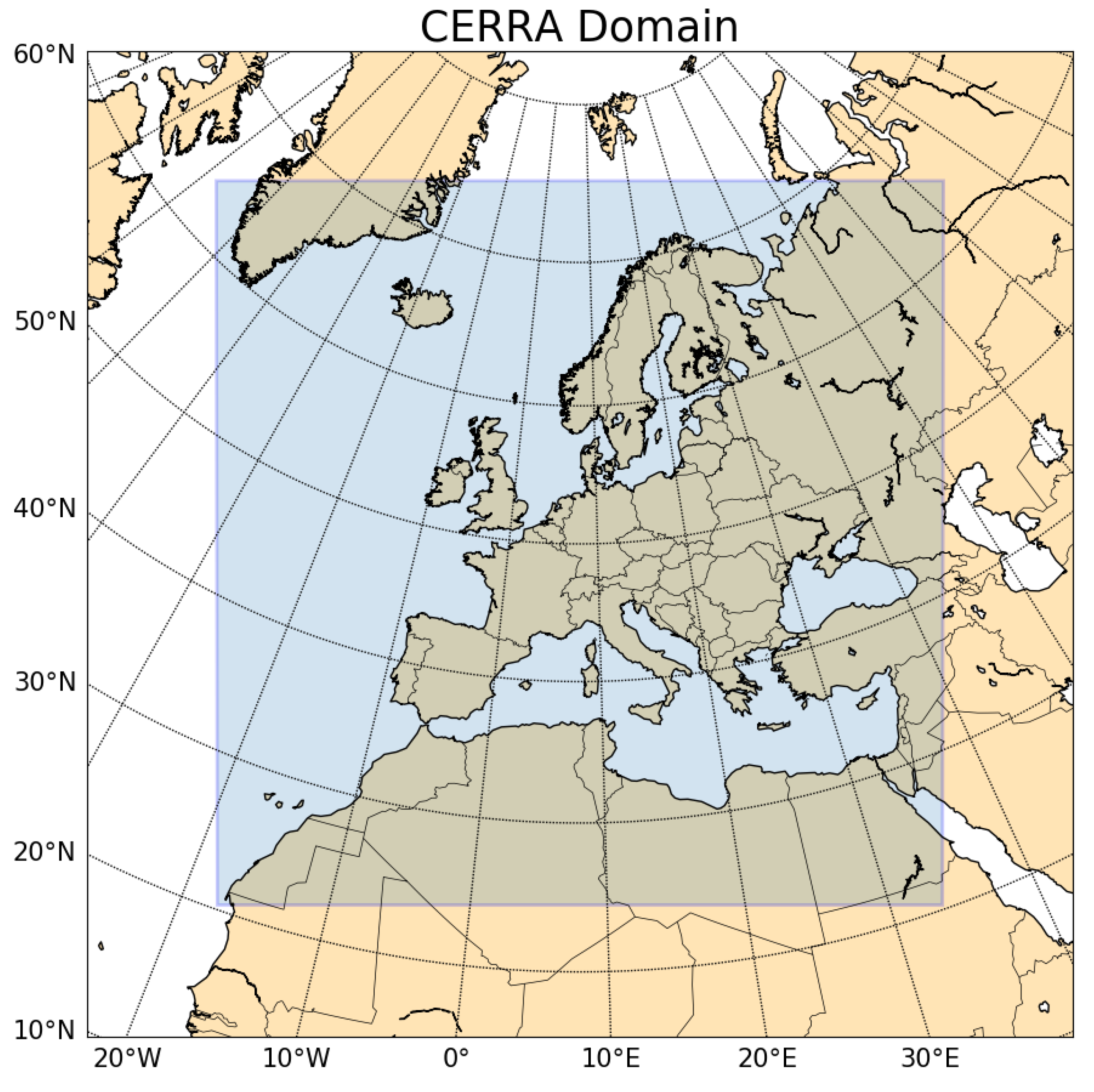
7]. It has a 5.5 km horizontal resolution with 106 vertical levels, spanning up to the model top of 1 hPa. The domain of CERRA covers Europe, Northern Africa and South-Eastern parts of Greenland, as shown in Figure 1.
The NWP is initialized with a 3D-VAR assimilation scheme for the upper air and an OI for the surface assimilation. The upper air analysis is computed through the minimization of the 3D-VAR cost function J, shown in Equation (1):
J ( x ) = 1 2 ( x x b ) T B 1 ( x x b ) + 1 2 ( y H ( x ) ) T R 1 ( y H ( x ) )
where x b is the background model state, y is the observation vector, H is the observation operator and B and R are the background and observation error covariance matrices, respectively. The NWP system has a 3-hourly cycling interval, where 30 h forecasts are produced at 00 and 12z assimilation times (cycles) and up to 6 h forecasts are generated at the 03, 09, 15 and 21z assimilation times. Unlike in the operational NWP systems, the number of observations assimilated in a reanalysis system is not limited by the observation cut-off time, since reanalysis is produced in hindsight relative to the time of observation measurement. Effectively, it has a longer assimilation window, which enables the assimilation of all observations measured within the 3-h assimilation window, including the reprocessed observation datasets.
An EDA system is coupled with the CERRA system to regularly update the B-Matrix, which is used in the deterministic 3D-VAR assimilation system. The B-Matrix consists of the climatological and the Ensemble Flow dependent (EFD) components, calculated from the EDA’s forecast differences [
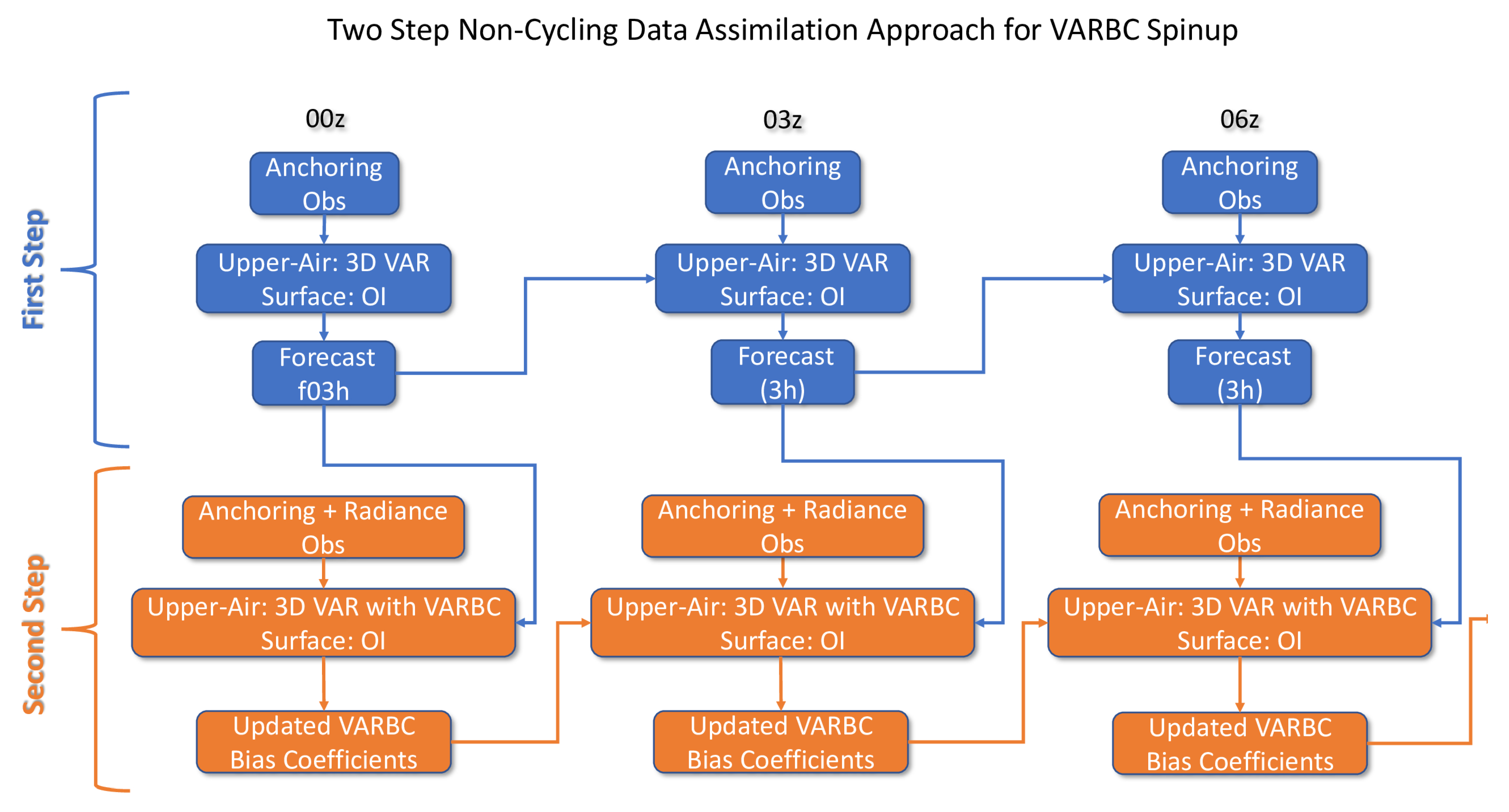
10]. The EDA system comprises 10 ensemble members, with 11 km horizontal resolution and has a 6 hourly cycling interval. Due to the different horizontal resolutions between the EDA and the deterministic system, the forecast differences were downscaled to the deterministic system’s 5.5 km resolution before being used to update the B-Matrix. Both systems use the ERA5 reanalysis as the lateral boundary conditions and assimilate the same types of observations. A workflow diagram in Figure 2 summarizes CERRA’s coupled systems.
An important focus during the development of the CERRA system was to assimilate as many observations that are available from the observing system throughout the reanalysis period. This was a challenging task as all the selected observation types from the 1980s to near-present have to be appropriately assimilated in the CERRA system. Table 1 shows the conventional observations that were chosen to be assimilated in the CERRA system, including local surface observations that are collected and quality controlled at the meteorological agencies in the Nordic countries (Norwegian Meteorological Institute (MET Norway), Danish Meteorological Institute (DMI), Swedish Meteorological and Hydrological Institute (SHMI), Finnish Meteorological Institute (FMI), Icelandic Meteorological Office (IMO)) and Météo France. Subsequently, the satellite observations selected to be assimilated are summarized in Table 2. It consists of the Microwave Sounding Unit (MSU), Advanced Microwave Sounding Unit-A and B (AMSU-A and AMSU-B), Microwave Humidity Sounder (MHS), Infrared Atmospheric Sounding Interferometer (IASI), Atmospheric Motion Vectors (AMV), GPS Radio Occultation (GPS-RO) and Ground-Based GNSS Zenith Total Delay (ZTD). The processing of the satellite radiance observations will be discussed more in detail in Section 3.

3. The Pre-Processing and Assimilation of the Radiance Observation

The CERRA system assimilates clear-sky radiance satellite observations, since added uncertainties from the assimilation of cloud contaminated observations can lead to degradation in forecast skills [25]. The CERRA system is equipped with a cloud detection scheme for high spectral resolution infrared sounders, developed by [26]. Their approach compares the observed spectra with the first-guess (FG) spectra of a cloud-free atmospheric state. The first guess departures are then ranked based on their sensitivity to the clouds and assigned an attitude in which complete overcast occurs for each particular channel. In the presence of monotonically increasing departures between the observed and computed spectrum, the cloud contaminated channels are then identified and removed. A similar approach described in [17,27] is applied for microwave sounder instruments in the CERRA system. Specifically, the first-guess departure threshold test compares the observed brightness temperature (BT) with the clear-sky FG brightness temperature and removes any radiance observations that have a departure higher than the predefined threshold. It is worth noting that many meteorological centres have made advancements in assimilating all-sky radiances [25,28]. The CERRA system does not include all-sky radiance assimilation, as such capabilities have not been yet implemented in the HARMONIE model framework.
The satellite instrument and channel selections in the assimilation of radiances were adopted from the HARMONIE system [17], shown in Table 3. They span from the early 1980s to near real-time, providing an adequate satellite coverage throughout the majority of the CERRA reanalysis. The satellite instruments include Microwave Sounding Unit (MSU), Advanced Microwave Sounding Unit-A/B (AMSU-A/B), Microwave Humidity Sounder (MHS) and Infrared Atmospheric Sounding Interferometer (IASI). In addition, the normalized weighting functions of all assimilated IASI channels are shown in Figure 3.

3.1. Assimilation of Surface Sensitive Radiance Observations

Unlike most of the microwave channels used in the CERRA system, AMSU-A channel 5 ( 53.596 ± 0.115 GHz) has a low peaking weighting function. Consequently, it has a higher sensitivity to near-surface properties, such as surface skin temperature and emissivity, as described by [29,30]. Significant advancement has been made in sea emissivity models to effectively assimilate surface-sensitive microwave channels over sea by [31,32]. However, the assimilation of radiance over land becomes more challenging as the surface emissivity over land (1.0) is higher compared to over sea (0.5–0.8) [29,30,33]. As a result, surface emissivity has a greater effect on the surface-sensitive microwave channels over land compared to the sea. In addition, the surface emissivity over land is highly dependent on the land-use type and roughness length, which can have greater spatial variability.
The CERRA system adopted two schemes from the HARMONIE system to utilize the surface emissivity and skin temperature and appropriately assimilate AMSU-A channel 5 ( 53.596 ± 0.115 GHz), as proposed by [29]. The first scheme ingests monthly mean emissivity atlases, which were computed offline based on AMSU-A/B near-nadir observations and atmospheric information from ECMWF 45-year reanalysis (ERA-40). When available, this scheme is preferred to take into account the seasonal variability of the emissivity. The second and alternative scheme calculates the emissivity dynamically within the data assimilation system by using the AMSU-A/B observations, while the atmospheric conditions are provided by the RTTOV model [34]. The impact of assimilating AMSU-A channel 5 ( 53.596 ± 0.115 GHz) on the CERRA system will be discussed in Section 5 and Section 6.

3.2. Thinning of Radiance Observations

Within the data assimilation framework, one assumes that the observation errors are not correlated. The correlation of observations errors is often substantial when assimilating networks of high-density observations such as radiance observations, resulting in sub-optimal analyses and forecasts. The correlation can exist spatially and inter-channel of satellite instruments, which can originate from radiative-transfer models, instrument design or calibration [22]. One approach for reducing the error correlation uses spatial thinning of the observations. Reference [35] showed improved forecast skills from the global Met Office NWP system by prescribing optimal spatial thinning for radiance observations. The author of [16] found the optimal thinning distance for the Advanced TIROS Operational Vertical Sounder (ATOVS) radiance assimilation in the ALADIN/Hungary limited area model (LAM) with significant impact on the short-range forecasts. The CERRA system adopted the thinning distance configuration from the HARMONIE system, which is applied using two steps [16,17,20,36]. While in the first step a minimum distance (defined by RMIND_RAD1C) between the active observations is guaranteed, the second step enforces a final prescribed (defined by “RFIND_RAD1C”) average distance. The summary of the thinning parameters for radiance observations is shown in Table 4.

3.3. Variational Bias Correction

Assimilating radiance observations with biases can be detrimental to the performance of the NWP system. The bias can originate from the radiative transfer model used as the observation operator in the assimilation of radiances. Other sources of bias include satellite instrumentation errors such as poor calibration, characterization and scanning position [18,19]. A variational bias correction (VARBC) scheme was implemented into NWP system by [37] in the common IFS (Integrated Forecast System), ARPEGE (Action de Recherche Petite Echelle Grande Echelle), ALADIN, and AROME (Application of Research to Operations at Mesoscale) variational data assimilation systems, which was later activated in the HARMONIE NWP system [20,36]. The advantage of the VARBC scheme is its ability to effectively remove potential bias dynamically, without requiring manual updating. This is especially beneficial in the framework of a reanalysis because less manual maintenance is needed to incorporate and monitor the biases correction from emerging satellites within the reanalysis’ lifespan [19]. In addition, the scheme is able to utilize anchoring observations such as radiosonde to better distinguish between the model bias and the bias from radiance observations [18]. As a result, the VARBC solely reduces the radiance biases while avoiding the radiance bias correction being drawn towards the model bias. A model without such capabilities can lead to the analysis drifting towards the model climate.
The VARBC scheme reduces the observation bias against its departure from the first guess model state. Originally, the observation departure is defined as Equation (2)
y H ( x )
where y the observation vector, x is the model state vector and H ( x ) is the observation operator, which is the RTTOV radiative transfer model for the case of radiance assimilation.
As defined by [38], the radiance observation bias is represented by the linear regression from a set of predictors p i , weighted by unknown bias predictor coefficients β i . Then the bias b ( x , β ) can be implemented into the observation operator H m ( x , β ) defined by Equation (3):
H m ( x , β ) = H ( x ) + b ( x , β ) = H ( x ) + n = 0 N β i p i ( x )
Consequently, the 3D-VAR cost function from Equation (1) becomes:
J ( x ) = 1 2 ( x x b ) T B 1 ( x x b ) + 1 2 ( y H m ( x ) ) T R 1 ( y H m ( x ) ) + 1 2 ( β β b ) T B β 1 ( β β b )
where β is the set of bias correction predictor coefficients for the current analysis, while β b represents the coefficients from the previous analysis cycle. Lastly, B β is the bias parameter background error covariance matrix, which is used to constrain the sensitivity on the bias correction to the new observations. It consists of error variances for the bias parameter σ β j 2 in the diagonal of the matrix shown in Equation (5) [37].
B β = d i a g ( σ β 1 2 , , σ β n 2 ) , w h e r e σ β j 2 = σ o j 2 N J j = 1 , n
where the error variances for the bias parameter are defined by the error variance of the radiance observations σ o j 2 , weighted by factor N j . Also, n is the number of used bias predictors.
The set of predictors consists of air-mass and scanning angle predictors [19,37]. In particular, the air-mass predictors are used to represent the errors from the radiative transfer model and are dependent on the atmospheric model state. The scanning angle predictors represent the bias associated with viewing angles relative to nadir. A list of the predictors used in the HARMONIE system can be found in Table 5. In general, predictors p0 to p7 are air mass predictors while p8 to p10 and p15 to p17 are scan angle predictors.
At the start of the operational life of each satellite and instrument, subsequent cycles of passive radiance assimilation is typically needed to train the bias correction coefficients to be representative of the radiance observation biases before the VARBC scheme effectively reduces the bias. For the purpose of this study, this procedure is called the VARBC spin-up period, where radiance observations are assimilated passively with active assimilation of anchoring observations such as radiosonde and GPS Radio Occultation observations. Given the satellite coverage within the CERRA’s domain and the predefined adaptiveness setting of the VARBC scheme, the VARBC spin-up period typically spans from 30 to 40 days for the bias coefficients to converge into stable and representative values and effectively correct the bias associated with radiance observations [20]. These newly computed bias correction coefficients will be used in active assimilation of radiance observations during the production of the CERRA dataset.
The adaptiveness of the VARBC scheme depends on the bias parameter background error covariance matrix, which can explicitly be controlled by the parameter N j . For example, a larger N j value in Equation (5) will reduce the error variances for the bias parameter β j and the diagonal of the bias parameter background error covariance matrix, thus decreasing the penalty in the bias correction term in the cost function from Equation (4), which allows the scheme to be more adaptive to the latest observations. However, an overly adaptive VARBC scheme risks sampling spurious bias signals that are not representative of the systematic biases. On the other hand, a smaller N j value will stiffen the scheme’s adaptiveness and result in a less responsive but a more stable convergence of the bias coefficients. The optimal N j value allows for a stable bias coefficient but is adaptive to change in the atmospheric conditions such as weather pattern fluctuation, seasonal and climatological variations. Reference [36] discussed the turning of a similar parameter for ATOVS in the context of the limited area model within the HARMONIE system and proposed an optimal value, which is also used in the CERRA system.
Throughout the development of the CERRA system, it was discovered that the passive assimilation of radiance observation in the VARBC spin-up period disables observation thinning, which results in ingesting relatively more observations than their active assimilation would have allowed. Specifically, substantially more radiance observations from higher spatial resolution instruments, such as IASI and MHS were ingested into the VARBC scheme. Consequently, the default N j values prescribed for IASI and MHS are insufficient to stabilize the convergence of the bias coefficient during the VARBC spin-up period. Rather than changing the values of N j for IASI and MHS, it was found more effective to actively assimilate them. This approach enables correct observation thinning and reduces the number of observations used in the VARBC scheme, which effectively stabilizes the convergence of the bias coefficients. However, the active assimilation of radiance observations with premature bias coefficients would cause the climate of the NWP system to drift towards the bias of radiance observation and degrade the representativeness of the bias coefficients. A possible solution consists of a two-step assimilation approach, illustrated in Figure 4. The first cycled assimilation procedure generates the first guess fields (3-h forecasts) with active assimilation of only conventional and anchoring observations. The second data assimilation procedure ingests the first guess field from the first procedure and assimilates the radiance observations with conventional/anchoring observations to update bias coefficients. Consequently, the non-cycling of the first guess field in the second procedure prevents the climate of the NWP system from drifting towards the bias of the radiance observations, while allowing for observation thinning through active assimilation of radiance during the VARBC spin-up period.

4. Impact of Variational Bias Correction

The VARBC coefficients were effectively spun up by adopting the two-step data assimilation approach. 
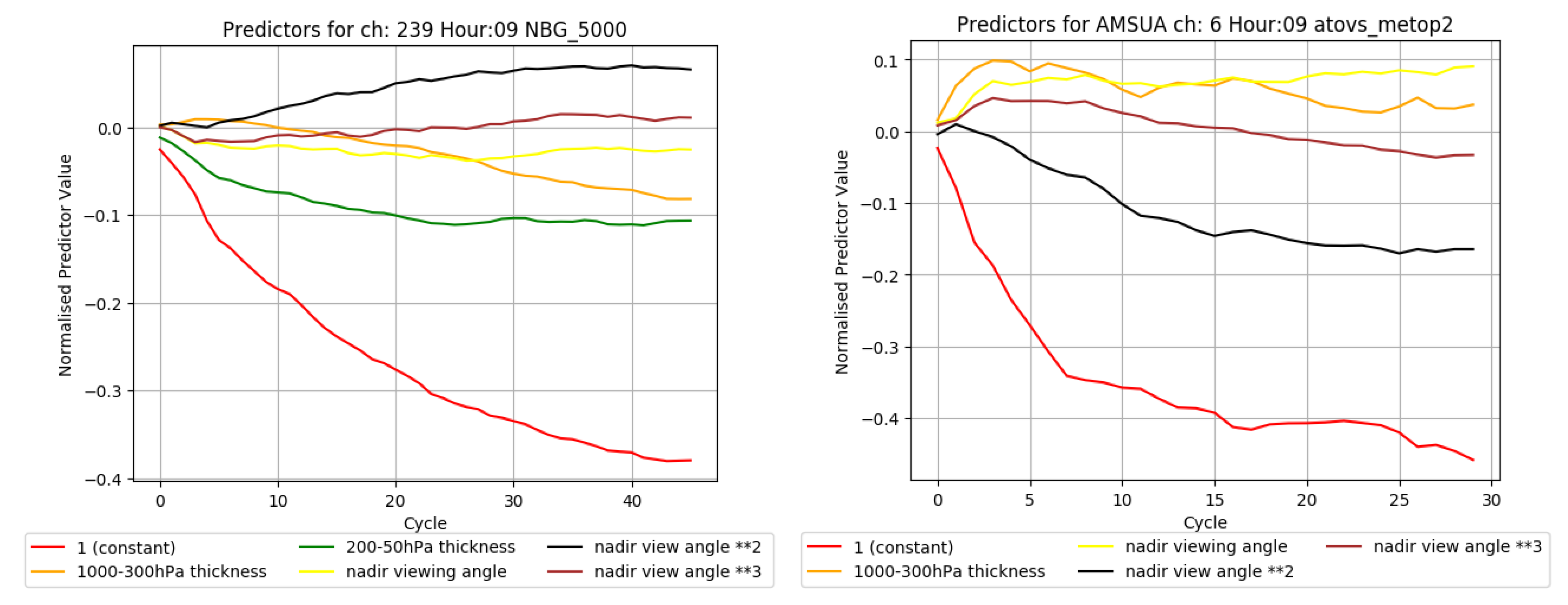
Figure 5 (left) illustrates the progression of the bias correction predictor coefficients during the 47-day VARBC spin up period for IASI channel 239 (704.50 cm 1 ) on MetOp-B at the 09 UTC cycle. This plot shows that the bias correction coefficients for most of the predictors have converged to stable values after approximately 43 days. In addition, Figure 6 (top-left) shows the evolution of the bias correction for the same channel over land and sea. The result reveals that observation minus first-guess (OMF) and observation minus analysis (OMA) biases slowly decrease towards 0 K from −0.43 and −0.2 K, respectively. After 43 days, the OMF and OMA biases have reduced to near-zero, which is consistent with the convergence of the bias correction predictor coefficients seen in Figure 5 (left). On the other hand, the non-corrected bias of OMF maintained approximately the same values, as expected. Similar results in Figure 5 (right) show the convergence of bias correction predictor coefficients for AMSU-A channel 6 ( 54.40 GHz) on MetOp-A after 15 days. Furthermore, the bias comparison in Figure 6 (top-right) indicates the OMF and OMA are reduced below 0.1K with the same period from −0.5 and −0.3 K, respectively. Overall, the two-step data assimilation procedure for the VARBC coefficients spin-up has been demonstrated to be effective in stabilizing the gradual reduction of the biases from the radiance observations and iteratively refining the bias coefficients during the spin-up period. Comparable results were found for the other IASI, AMSU-A, and AMSU-B/MHS channels.
Once the bias coefficients from the VARBC spin-up period are considered to be representative of the biases associated with the assimilated radiance observations, it can be used in the full NWP system. Unlike the VARBC spin-up procedures, the first guess in the operational CERRA system is cycled in the subsequent assimilation time, as described in Figure 2. A 21-day experiment with the full CERRA system was conducted to examine the performance of the VARBC scheme and the impact of the radiance assimilation. Figure 7 (top-left) illustrates the time series of non-corrected OMF bias, corrected OMF bias and OMA bias for IASI channel 296 (718.75 cm 1 ) on MetOp-B at the 9 UTC cycle. This result shows a reduction between the non-corrected OMF biases and the corrected OMF bias, decreasing from 0.2 K to less than 0.1 K. One can also see that the biases are relatively stable and have minimal fluctuation throughout the period of the experiment. This result is consistent with relatively stable bias predictor coefficients found in Figure 7 (right). Overall, these findings suggest that the VARBC coefficients that were computed during the spin-up period can be effectively used in the full NWP system for a long-term experiment and production of the CERRA dataset. Similar results were found for AMSUA, AMSU-B and MHS instruments.
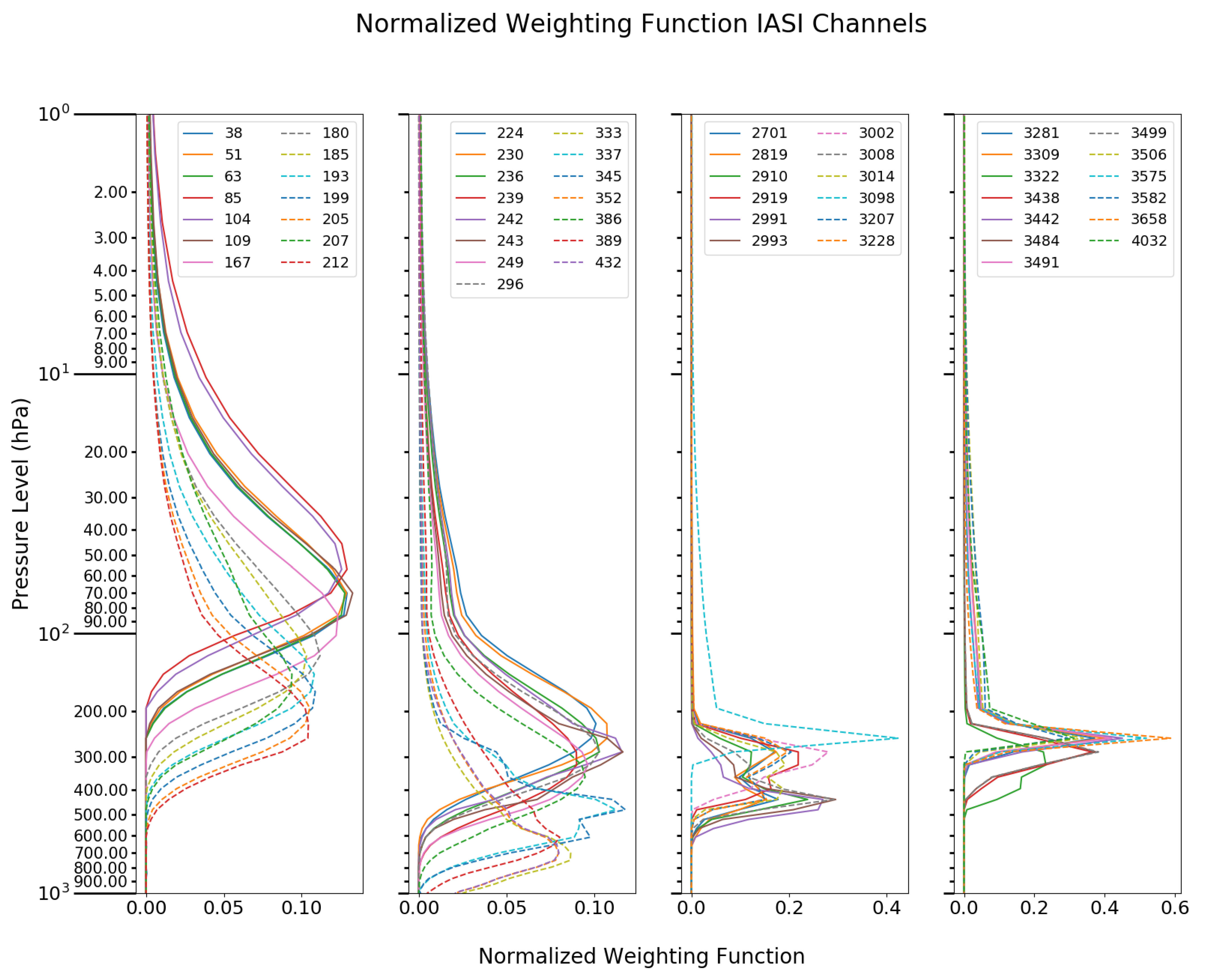
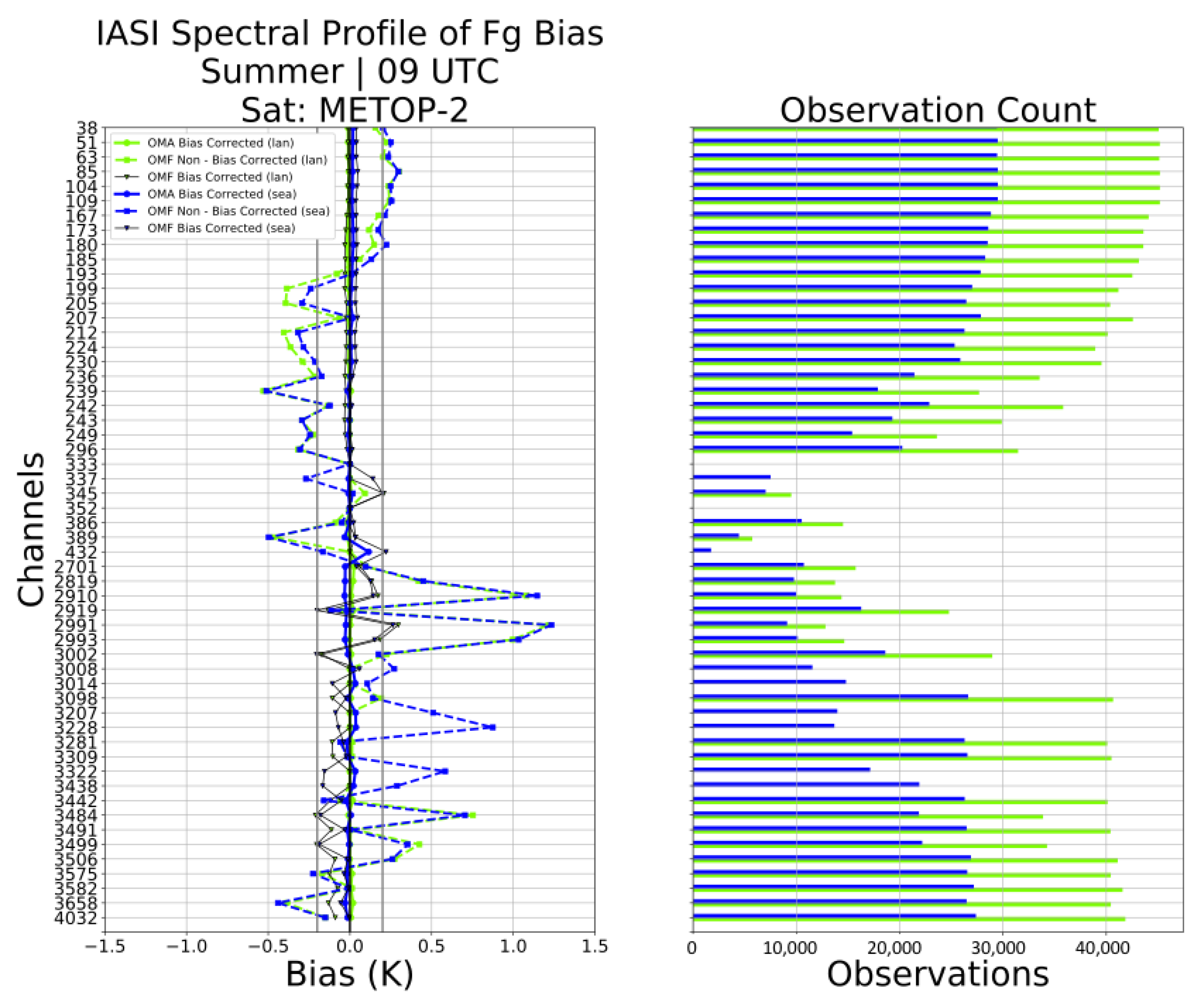
In order to have a more comprehensive approach to analyze the bias for all of the 55 assimilated IASI channels, Figure 8 shows the spectral profile of the non-corrected OMF bias, corrected OMF bias and OMA bias for all of the selected IASI channels on MetOp-A at 9 UTC assimilation time. Generally, the channels with relatively high peaking weighting functions from CO 2 absorption bands (Channel 38 to 193; 654.25 to 693.00 cm 1 ) have non-corrected OMF biases between 0.2 to 0.5 K. The lower peaking channels (Channel 199–432; 694.50 to 752.75 cm 1 ) have smaller non-corrected OMF biases, fluctuating close to 0.2 K. Lastly, the respective values for the channels in the water absorption bands (Channel 2701–4032; 1320.00 to 1652.75 cm 1 ) are as high as 1.2 K. As expected, the corrected OMF and OMA biases for channels from CO 2 absorption bands are systematically close to zero. However, few channels in the water absorption band have higher bias-corrected OMF, reaching up to 2.3 K. Due to this high bias-corrected OMF bias, the observation errors were configured to be greater compared to the other absorption bands to reduce the impact on the analyses and forecasts [39]. Similar results are also seen for other cycles that assimilate IASI observations.

5. Relative Impact of Radiance Observations in CERRA Analyses and Forecast

The relative impact of assimilating radiance observations on CERRA analyses and forecasts are studied using two diagnostic metrics, namely the Degrees of Freedom for Signal (DFS) [40] and the Moist Total Energy Norm (MTEN) [41]. The DFS and MTEN compute, respectively, the sensitivity of the analysis and forecast systems to the individual observation types used in the data assimilation.

5.1. The Sensitivity of the CERRA Analyses to the Radiance Observations

The DFS provides an insight into the sensitivity of the data assimilation system to the individual observation type, as introduced by [40]. This diagnostic tool has been used in various studies to examine the impact of observations [3,20,30,42,43]. It is interpreted as the trace of the gradient of the analysis in observation space with respect to the observation vector, which can be approximated from the observation vector y , the perturbed observation vector y ^ , analysis x a , the analysis produced from the perturbed observations x ^ a , background state x b and the observation error covariance matrix R , as shown in Equation (6).
D F S = T r [ H i x a y i o ] = y i o O b s e r v a t i o n s H i x a y i o ( y ^ y ) R 1 ( ( H ( x ^ a x b ) H ( x a x b ) )
Figure 9 illustrates the absolute DFS, characterizing the impacts of each type of observation assimilated in the CERRA system on 26 December 2017. This comparison shows that the aircraft wind measurements (AIREP-U) have the highest impact on the analysis, while slightly lower effects are observed for the atmospheric motion vector (AMV), Scattometer (SCATT) and aircraft temperature measurements (AIREP-T). Weaker influences are also seen from radiosonde observations, which can be attributed to its availability mainly at 00 UTC and 12 UTC, whereas the other observations are also available in other assimilation times. In other words, the impact of radiosonde would be ranked higher if the absolute DFS was evaluated for 00 and 12 UTC assimilation times individually, rather than computing these results for all eight assimilation times simultaneously. Comparable results are found among the radiance observations with IASI having the highest absolute DFS, while AMUS-B and AMSU-A rank behind. Overall, the absolute DFS for radiance observations are generally smaller than conventional observations. It is worth noting that the same comparison was made for 2 January 2018, 30 May 2018 and 11 June 2018 with comparable results.

5.2. The Relative Sensitivity of the CERRA Forecasts to the Observation

One can infer the sensitivity of the forecast model from a subset of observations by examining the loss of moist total energy norm when removing them from the assimilation system [20]. Essentially, the MTEN can be expressed as a cost function J, which is computed through a comparison between the control forecast x t ctr that was initialized with the assimilation of all observations versus the forecast x t i that was initialized without the assimilation of the subset of observations, as shown in Equation (7). The forecast time is defined by t, while i represents the index of the observations subset to be removed and studied. Also, a localization operator P can be used to examine the sensitivity of the forecast model within a specific subset of the model domain, such as between particular model levels, spatial regions, and/or sea/land masks [41,44].
J = < P ( x t i x t ctr ) , P ( x t i x t ctr ) > = η 1 η o D ( u 2 + v 2 + C p T r T 2 + R T p r 2 p 2 + L 2 C p T r q 2 ) p r η d η d D
where T, q, p, u and v represent temperature, specific humidity, surface pressure; u and v wind components, respectively. In addition, p r , T r , c p , R, L represent the reference pressure, reference temperature, specific heat at constant pressure, gas constant for dry air and latent heat condensation. Depending on the localization operator P, the energy norm can be integrated between vertical levels from the native model levels η 0 and η 1 and/or across subsections of the model domain. One should note that MTEN is sensitive to present synoptic patterns and observation coverage from the various assimilation times. Therefore, it is expected to have slightly varied results for different periods [17,20].
Figure 10 depicts the vertical profiles of MTEN showing the CERRA forecast sensitivity to aircraft, radiosonde, IASI, AMSU-B/MHS, AMSU-A and only channel 5 AMSU-A ( 53.596 ± 0.115 GHz) observations. The comparison consists of MTEN vertical profiles for 3, 12 and 24-h forecasts that are initialized at 12 UTC on 26 January 2018 and 30 May 2018. Overall, the aircraft observations have the strongest MTEN for the 3, 12 and 24-h forecasts, suggesting that the aircraft observations have the greatest impact, especially for the upper troposphere and the tropopause. Subsequently, radiosonde observations have the second greatest impact, while smaller influence was observed for radiance observations, especially for the 3-h forecast. However, the difference in impact between the upper-air conventional observations and the radiance observation reduces for the 12 and 24-h forecasts. This implies that the impact from the assimilated radiance observations is more predominant in the longer forecasts than shorter forecast lengths. Also, the results show that the assimilation of the AMSU-A channel 5 ( 53.596 ± 0.115 GHz) with the utilization of emissivity and skin temperature has considerable impact compared to all channels of AMSU-A, especially within the lower troposphere for all forecast lengths. In addition, the impact of AMSU-A and MHS for 3 and 12-h forecasts extends further towards the lower troposphere, while the influence of IASI is more pronounced for the mid-troposphere. This can be attributed to sensitivity in the atmosphere with respect to the weighting functions of the selected channels from the three satellite instruments. These findings are consistent with MTEN comparisons that were computed for additional dates, including 2 January 2018, 30 May 2018 and 11 June 2018 (not shown). However, the ranking of the impacts among the radiance observations changes for the different initialization times and forecast lengths due to the evolving weather patterns and the varying observations coverage from the passing satellite platforms at each individual assimilation time.

6. Impact of Radiance Observations through Verification Scores

As previously mentioned, DFS and MTEN diagnostic metrics provide the relative impact of the radiance observations on analysis and forecast, but it does not provide information on the quality of the impact (positive or negative). Consequently, the impact from a subset of observations can be further assessed by performing data denial Observing System Experiments (OSEs), where the observations of interest are removed from the full assimilation system [39,45,46,47]. The produced analyses and forecasts (impact experiments) are then compared with their counterpart from the full (control) assimilation system to assess the changes in the analyses and forecasts through verification scores. It is essential to ensure that the difference in the quality of the analysis and forecast between the control and the impact experiments are significant and not attributed to the chaotic variability in the atmosphere. This issue becomes more critical for regional NWP systems and with relatively shorter experiment periods because of the fewer available observation samplings used in the verification. Based on the Student’s T-test, significant tests are used to compute the normalized mean root mean square error (RMSE) difference, where the temporal auto-correlation is corrected using the first-order auto-regressive process, as discussed in [48] and used by [17,20]. It is worth noting that the significance of the statistical results are only valid for the relatively short duration of the experimental period, within the larger reanalysis period. The verifications focus on the changes in the atmospheric part of the CERRA analyses and forecasts, which verifies the analyses and forecasts against radiosonde observations at 00 and 12 UTC, while providing insight on the significance of the results.
The first OSE (“NoRAD”) was conducted to assess the impact of all radiance observations by removing them from the full assimilation system. The verification scores of the analyses and forecasts were then compared against the control experiment (“Allsat”), which consisted of an assimilation system with all radiance observations. The experiments were performed for both the summer and winter periods, spanning from 23 December 2017 to 16 January 2018 and 28 May to 19 June 2018, respectively. In addition, an eight days model warm-up period was applied to all the experiments, prior to the verification periods. Figure 11 and Figure 12 illustrate the vertical profile of the normalized mean RMSE Difference at 90% confidence for geopotential height between “AllSat” and “NoRAD” for the summer and winter periods, respectively. Negative values in the figures indicate the normalized mean RMSE for “AllSat” experiment is less than that of the impact experiment, suggesting the errors of the forecast or analysis is reduced when the subset of observations is included in the full assimilation system. In other words, it can also be interpreted as the deterioration of the analysis and forecast caused by removing the subset of observations from the full system, indicating that the subset of observations has a positive impact. This study focuses on the impact on Geopotential height because of the high statistical significance across many of the analysis times and forecast lengths. Such high statistical significant results are not as distinct for the other verified variables.
From the winter period in Figure 11, the assimilation of all radiance observations (green line) has minimal impact on the analyses (left and middle plots), while increasing the normalized mean RMSE by 1–2% between 200–100 hPa and below 500 hPa on the 3-h forecasts from 09 UTC (right plot). On the other hand, the 24-h forecast from 12 UTC has an error reduction by 1.5 to 2.5% below 300 hPA, while the neutral impact is observed above 200 hPa (not shown). The summer case in 
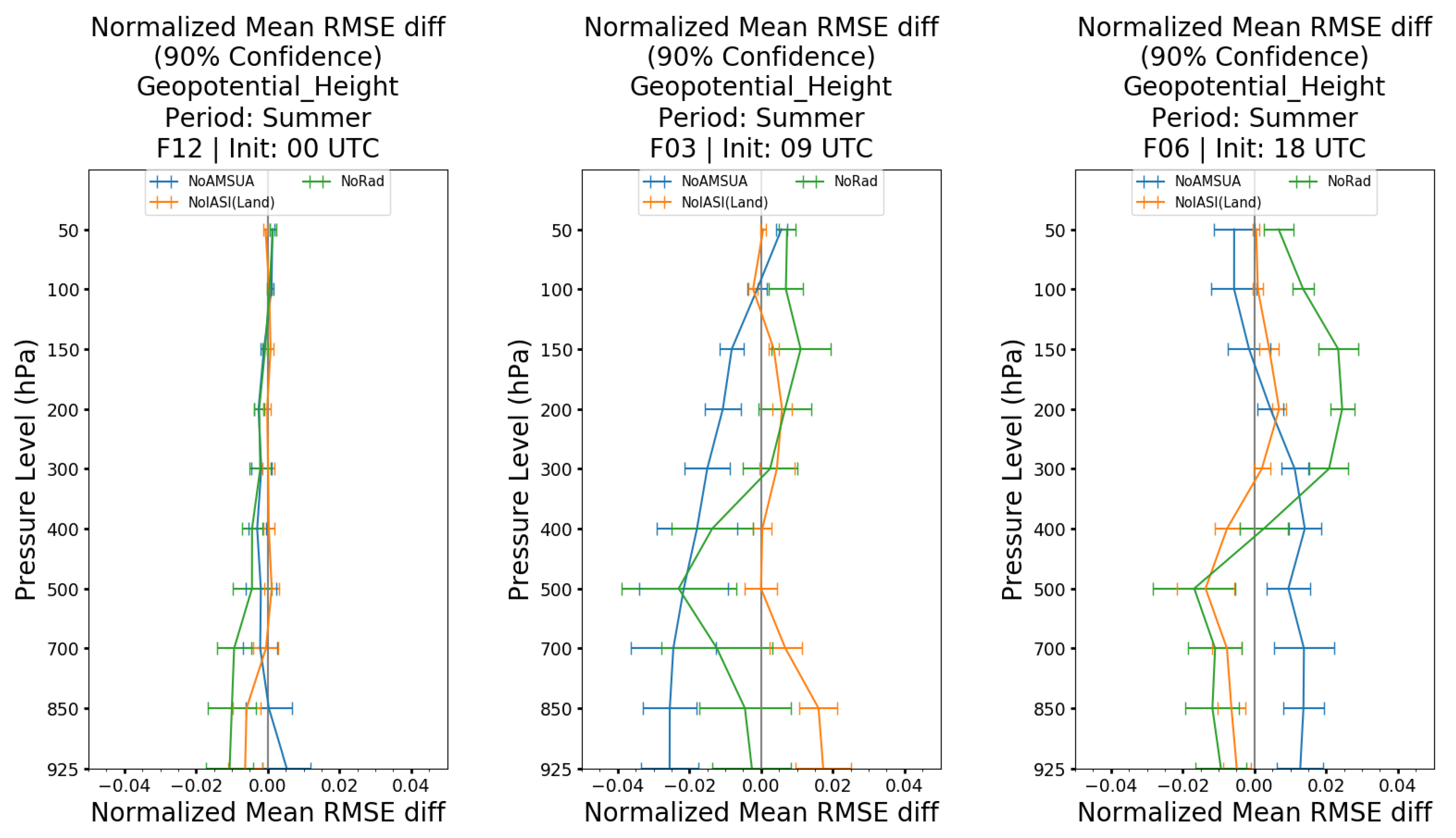
Figure 12 illustrates a minimal impact on the analyses at 12 UTC. There is a positive impact on the 3-h forecasts from 09 UTC below 400 hPa with 2% reduction in RMSE reduction with significance at 500 hPa, although 1% significant degradation is also observed between 150 and 50 hPa. In addition, the impact on the 6-h forecasts from the 18 UTC cycle shows a significant improvement of 1% below 500 hPa, but a negative impact up to 2% for 300 hPa and above. Such negative impact in the upper troposphere and stratosphere is not observed on the other forecast lengths and assimilation times, which prompted further examination to determine the cause of this phenomenon.
In the initial investigation, several one-day OSEs were conducted for AMSU-A, AMSUB/MHS and IASI for both the summer and winter periods. A comparison of the geopotential height forecast fields at various vertical levels showed that AMSU-A and IASI had the strongest impact, while minimal influence was observed from AMSUB/MHS (not shown). From the short experiments, the assimilation of AMUS-A typically has a positive impact when verified against radiosonde observations, while the impact of IASI was inconclusive. This indistinctive impact from IASI may be contributed by the CERRA system’s inability to characterize skin temperature and emissivity for the assimilation surface-sensitive IASI channels over land. ECMWF’s global NWP system had similar constraints, resulting in rejecting all IASI observations over land in their assimilation system [49]. This issue in the CERRA system was initially addressed by rejecting predominant surface-sensitive channels, but a few relatively low peaking channels are still assimilated, which can lead to additional uncertainties into the system. Due to the shortened experiments, the results can be questionable without insight on its significance.
In order to substantiate this hypothesis in a robust manner with significance, two additional 21+ days OSEs were performed for AMSU-A (“NoAMSUA”) and IASI observations over land (“NoIASI(Land)”) for the summer and winter periods. Similar to “NoRad” comparison, the vertical profiles of the normalized geopotential height mean RMSE difference at 90% confidence for “AllSat” minus “NoAMSUA” and “AllSat” minus “NoIASI(Land)” are shown in Figure 11 (Winter) and 
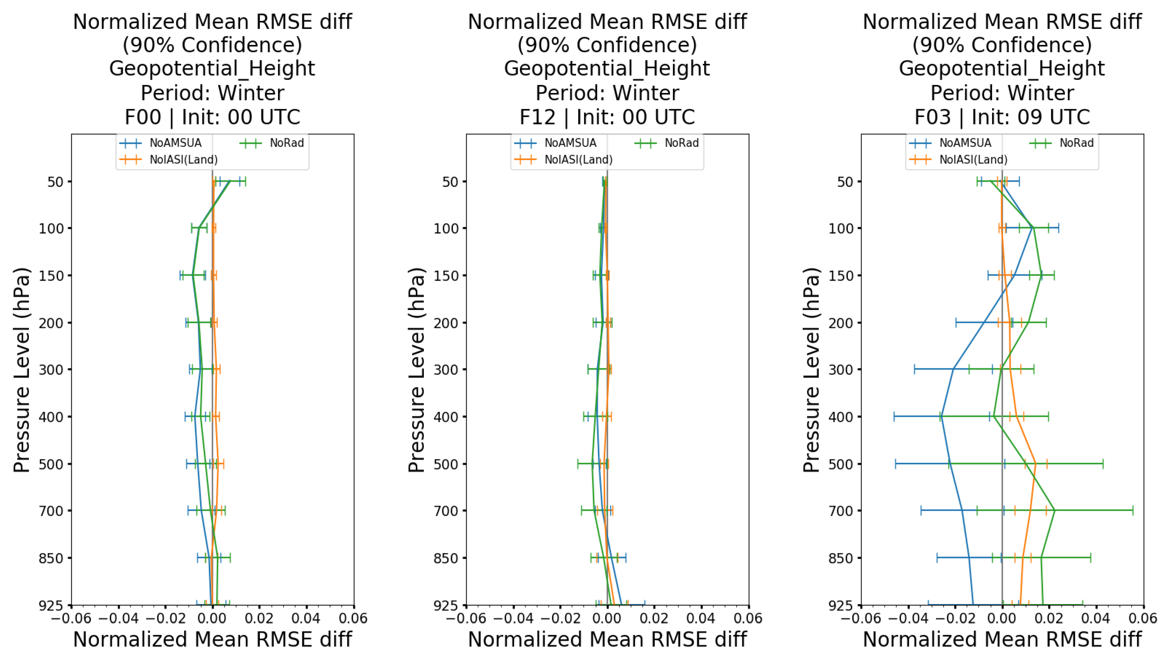
Figure 12 (Summer). In the winter case (Figure 11), the assimilation of AMSU-A reduced the error by 0.5 to 1% with significance on the analyses at 00 and 12 UTC (left and middle plots). Furthermore, there is also an error reduction of 1.5 to 2% at 400 and 300 hPa on the 3-h forecasts from 09 UTC (right plot). However, the assimilation of IASI observation over land increased the error by 0.5 to 1.5% for the 3-h forecasts, initialized at 09 UTC. The results in the summer case (Figure 12) indicate that the assimilation of AMSU-A reduced the error of the analyses at 12 UTC by 1 to 1.5% for pressure levels between 925 to 500 hPa (left plot). The error reduction is also seen below 150 hPa for the 3-h forecast from 09 UTC by 1 to 2.5% (middle plot). Furthermore, the assimilation of IASI over land increased the error by 0.5 to 1.8% of the analysis at 00 UTC (not shown) and of that of 3-h forecasts from 09 UTC (middle plot). The results from the 6-h forecasts, initialized at 18 UTC showed an improvement in the error of 0.5 to 1% for pressure levels between 300 and 925 hPa but deteriorated the forecast at 200 and 100 hPa (right plot).
In the summer case, the negative impacts on 6-h forecasts from 18 UTC cycle are highly correlated between “NoRad” and “NoIASI(Land)” experiments within the upper troposphere and the stratosphere. By rejecting the IASI observations over land, the negative impact in the upper levels is slightly reduced, although the observed positive impact in the lower troposphere also reduced well. Further, we also observed that the positive impacts on other forecast lengths and assimilation times are enlarged. Overall, the results suggest that the rejection of IASI observations over land improves the accuracy of the analyses and forecasts. However, the residual negative impact is still present for the upper troposphere and stratosphere in the case of 6-h forecasts from 18 UTC.
Further investigations were conducted to determine the cause of the upper level negative impact from assimilating all radiance observations for the 6-h forecast at 18 UTC, during the summer period. Among various possibilities, the radiance observation error correlation and the configuration of the thinning distance for radiance assimilation were examined. One can use a method proposed by [
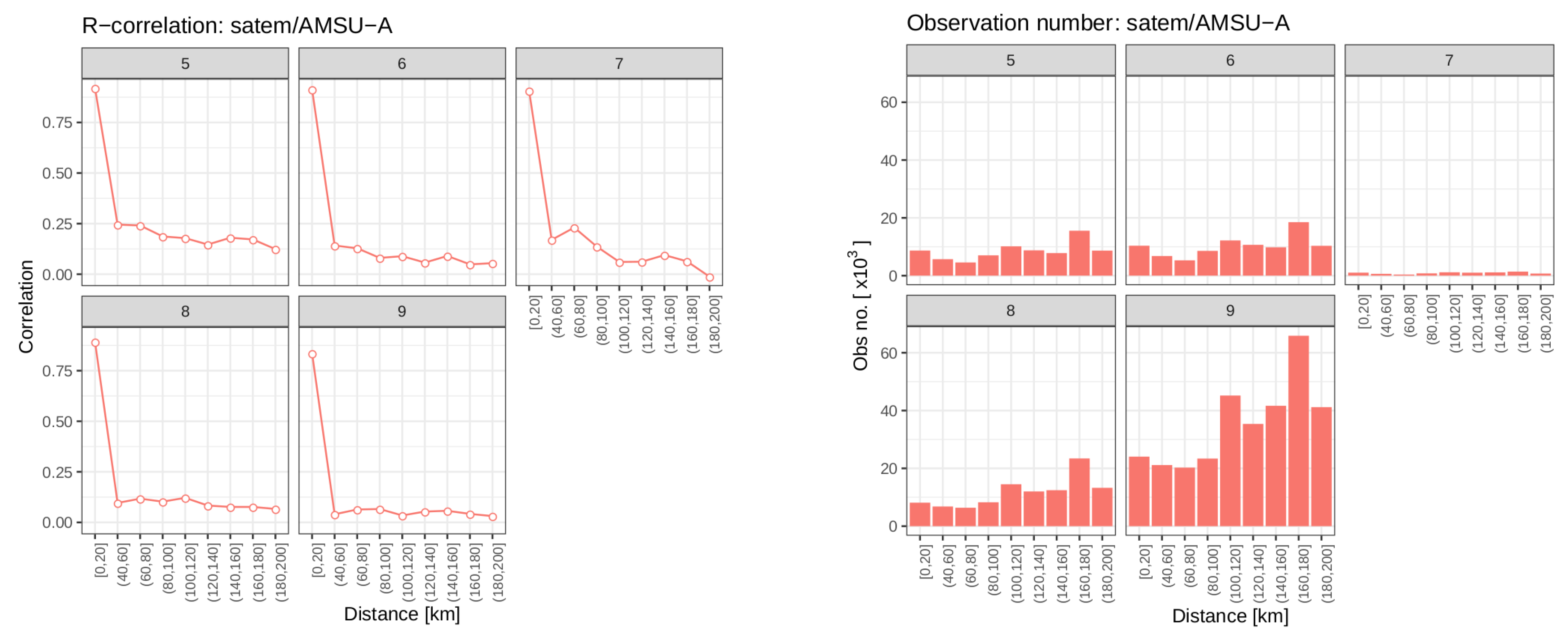
21] (referred to as the Desroziers method hereafter) to derive the spatial correlation of observation errors, which is computed based on the observation and analysis departures in observation space. This approach was used during the development of the CERRA system to study the appropriate thinning distance for the assimilation of ATOVS and IASI observations. Based on Desroziers method, Figure 13 illustrates the observation error correlation against the spatial separation distance for AMSU-A channels 5–9 ( 53.596 ± 0.115 57.290 GHz). The results for channels 6, 8 and 9 (54.40, 57.290 and 55.50 GHz) suggest that the correlation of observation error has reached lower than the threshold of 0.2. This value of the threshold for an optimal thinning distance was suggested by [23]. However, the correlation for channel 5 ( 53.596 ± 0.115 GHz) remains to be greater than this threshold for the separation distances less than between 80 and 100 km. This is also seen from [22], where channel 5 ( 53.596 ± 0.115 GHz) has a relatively higher correlation due to its sensitivity to the surface. Lastly, channel 7 ( 54.94 GHz) has a less conclusive result as the correlation fluctuates over the threshold from a distance of 40 to 100 km, which can be attributed to the significantly fewer number of observations used in the computation, compared with that of the other channels. Furthermore, the AMSU-B/MHS comparison suggests that the observation error correlation for channel 4 ( 183.31 ± 3.0 GHz) remains slightly above 0.2 from 40–60 km (not shown). Similarly, few IASI channels in moisture absorption bands and high peaking CO 2 absorption bands are highly correlated (0.25 to 0.35) for separation distances greater than 120–200 km, including channels 104, 180, 2991, 3098, 3309 and 3506 ( 670.75 , 689.75 , 1392.50 , 1419.25 , 1472.00 and 1521.25 cm−1) (not shown). Overall, the results suggest that the currently prescribed thinning distance parameters for the assimilation of radiance observations might not be appropriate and therefore further tuning is needed.
In order to address the high observation error correlation for radiance observations in the CERRA system, one can increase the thinning distance and/or inflate the observation error for these observations [22,50]. Consequently, three impact experiments with different thinning distance configurations for radiance observations were conducted, while rejecting IASI channels 104, 180, 2991, 3098, 3309 and 3506, due to its highly correlated observation errors. An additional impact experiment (“AMSUA Sigma_O x2”) was performed with the default thinning distance setting, but inflating the observations errors for AMSU-A observations by a factor of two. Lastly, a control experiment (Thin_60_80 km) with the default configuration described in Table 4 was conducted. A summary of the five experiments with different configurations is shown in Table 6.
The five experiments were conducted to produce the single-cycle 6-h forecast from 18 UTC 30 May 2018 to further address the negative impact of all radiance observations on the upper troposphere and the stratosphere. This investigation is limited to a single forecast cycle due to the limited computation resources. 
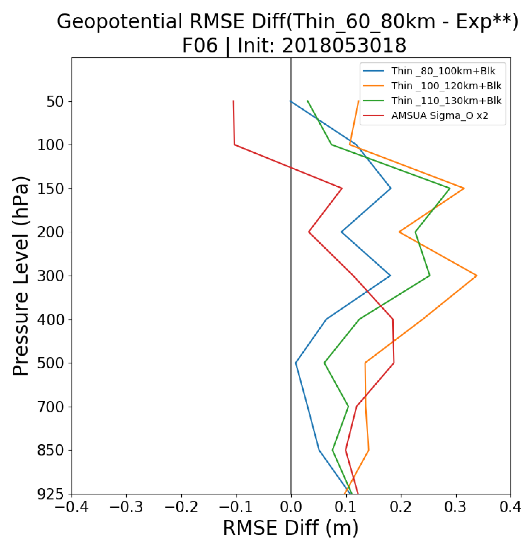
Figure 14 depicts a vertical profile of geopotential height RMSE difference between the control experiment (“Thin_60_80 km”) and the (four) impact experiments for the 6-h forecast, initialized at 18 UTC on 30 May 2018. The forecasts are verified against radiosonde observations. Positive values indicate that the control experiment with the default settings has larger RMSE than the impact experiments, suggesting that the impact experiments with the new setting improve the forecast’s accuracy. The results show all three impact experiments with increased thinning distances have lower RMSE than the control experiment, especially for the upper troposphere. Specifically, the “Thin_100_120 km + Blk” experiment has the lowest RMSE (largest difference compared to the control), while further increasing the thinning distance in the “Thin_110_130 km + Blk” experiment did not result in an additional RMSE reduction. Lastly, inflating the observation errors for AMSU-A radiance observations by two times in the “AMSUA Sigma_O x2” experiment reduced the forecast error to the level of that of the “Thin_100_120 km + Blk” experiment below 500 hPa. However, the reduction in forecast errors was significantly reduced for atmosphere aloft. One should consider these findings with caution since the results have minimal significance when only a single cycle was used in this investigation. Therefore, longer impact experiments with increased thinning distance are discussed in later sections, where the “Thin_100_120 km + Blk” experiment was conducted for a longer period during both the summer and winter seasons.
The results in Figure 11, Figure 12, Figure 13 and Figure 14 from the previous discussions suggest that the accuracy of the analyses and forecasts can be further improved by tuning the thinning distance for radiance observations and also by rejecting the IASI observations over land. In order to verify the effects of these modifications, three experiments were conducted and compared against the control experiment (“NoRad”), where all radiance observations were removed from the full assimilation system. The first impact experiment (“AllSat”) follows the default setting of the CERRA system, where all observations are assimilated. The second experiment (“noIASI(Land)”) adopts the same configuration as the “AllSat” experiment but rejects the IASI observations over land. Lastly, the third impact experiment (“Thin(100–120 km)_noIASI(Land)”) also follows the configuration from the “AllSat” experiment, but does not assimilate IASI observations over land and increased the thinning distance for the radiance observation to RMIND_RAD1C = 100 km and RFIND_RAD1C = 120 km.
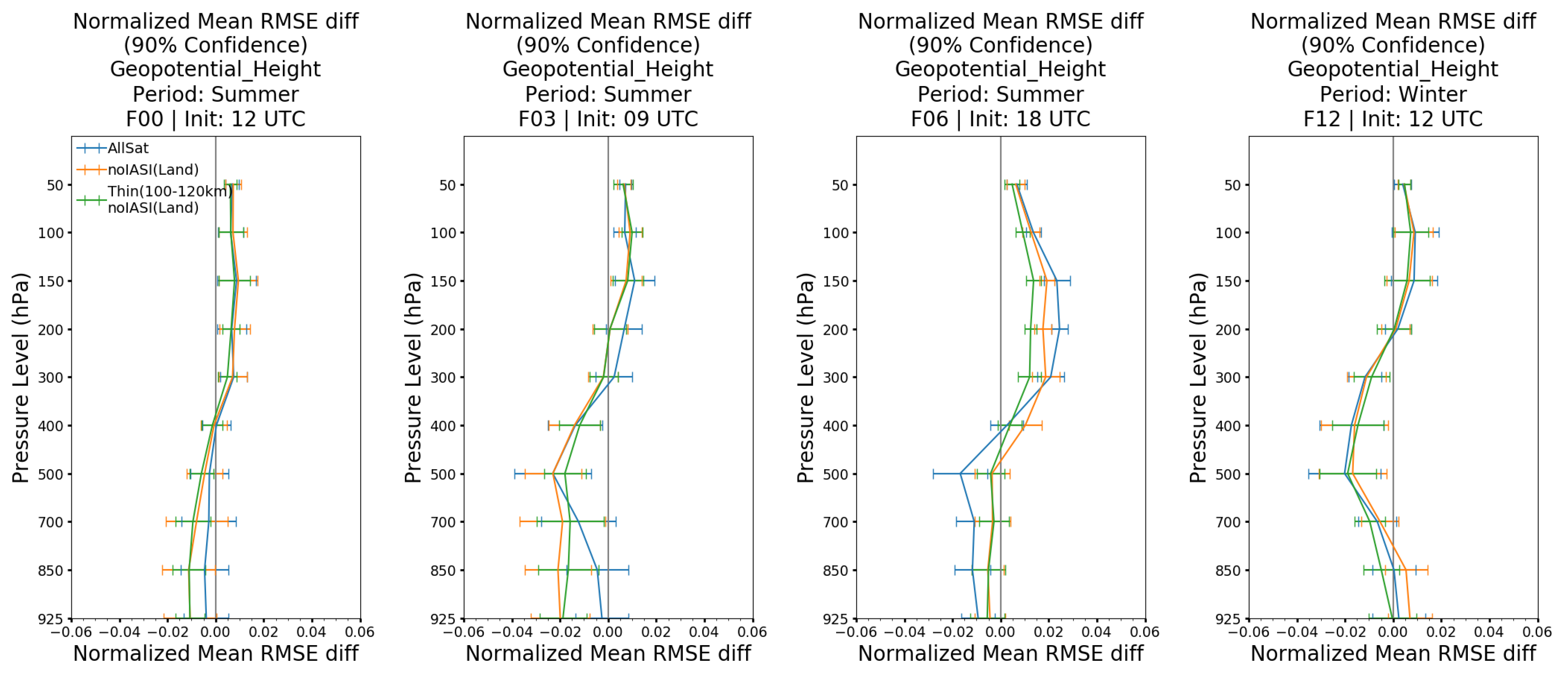
Figure 15 and Figure 16 illustrate the vertical profile of the normalized mean Root Mean Square Error Difference (at 90% Confidence) for geopotential height, comparing the impact experiments minus the control experiment using verification against radiosondes. Negative differences indicate a normalized mean RMSE reduction when compared against the control experiment (NoRad), suggesting that the impact experiments produce more accurate analyses and forecasts compared to the control experiment.
The winter case results in Figure 15 show that the “Allsat” experiment provides the smallest normalized mean RMSE reduction against the “NoRad”, while increases in forecast error were also observed in some cases. On the other hand, “Thin(100–120 km)_noIASI(Land)” generally has the largest reduction in normalized mean RMSE, followed by “noIASI(Land)”. Specifically, the 3-h forecast from 09 UTC has an approximately 2% error reduction for “Thin(100–120 km)_noIASI(Land)” compared to “AllSat” for pressure levels between 925 to 700 hPa. On the contrary, “noIASI(Land)” has only roughly 1% error reduction compared to “AllSat”. Although a more modest error difference is seen for other cases, it is evident that the radiance assimilation setup in “Thin(100–120 km)_noIASI(Land)” and “noIASI(Land)” both lead to improved accuracy in analyses and forecasts of geopotential height, compared to “AllSat”. Nevertheless, “Thin(100–120 km)_noIASI(Land)” produced the best results for the winter period. The large reduction in normalized mean RMSE from “Thin(100–120 km)_noIASI(Land)” is less predominant in the summer case, shown in Figure 16. In particular, there is minimal difference in reduction between “Thin(100–120 km)_noIASI(Land)” and “noIASI(Land)”, but both comparisons have up to 1 to 2% normalized mean RMSE reduction compared to “Allsat” for the analyses at 12 UTC and 3-h forecasts from 03 and 21 UTC cycles. Furthermore, “Thin(100–120 km)_noIASI(Land)” has the largest error reduction of 1.5% for the 6-h forecasts at 18 UTC above 300 hPa. However, the positive impact for the lower troposphere is slightly reduced compared to “AllSat”. Lastly, “Thin(100–120 km)_noIASI(Land)” and “noIASI(Land)” marginally degrade the 12-h forecast from 12 UTC. Overall, there is an added benefit by rejecting the IASI observation over land and/or increasing the thinning distance for radiance observations, leading to improvements in the accuracy of the analyses and 3-h forecasts.
By establishing “Thin(100–120 km)_noIASI(Land)” as the most optimal assimilation configuration for radiance observations in the CERRA system, one can further evaluate its performance against the control experiment “NoRad”. From the winter case results, the analyses at 12 UTC and the 3-h forecasts from 09 and 21 UTC suggest that “Thin(100–120 km)_noIASI(Land)” have a neutral impact compared to “NoRad” below 200 hPa. However, a positive impact is seen for the 12 and 24-h forecasts, initialized at 12 UTC, where there is a normalized mean RMSE Difference of −1 to −2% for the mid-troposphere. The analysis and 3-h forecast below 400 hPa from 09 and 12 UTC also showed improvement by 0.5 to 1% and 1.5 to 2%, respectively. Similarly, the 12-h forecasts from 12 UTC improved by 1 to 1.5% for 400 and 500 hPa. The negative impact seen from the “AllSat” experiment was reduced by 1% for atmospheric layers above 500 hPa, with the modification of configuration in the “Thin(100–120 km)_noIASI(Land)” experiment. However, the positive impact below 500 hPa in the “AllSat” experiment was reduced by 0.5% from the same changes in configuration.

7. Discussion and Conclusions

This study has considered some of the challenges of satellite radiance assimilation, while demonstrating its impact on the CERRA system. It was discovered that the use of passive assimilation during the VARBC bias coefficient spin-up was not appropriate for high spatial satellite instruments with high-density observation, within the framework of the limited area model. The two-step assimilation alternative approach was able to effectively spin-up the VARBC bias coefficients to be suitable for use in the CERRA production system.
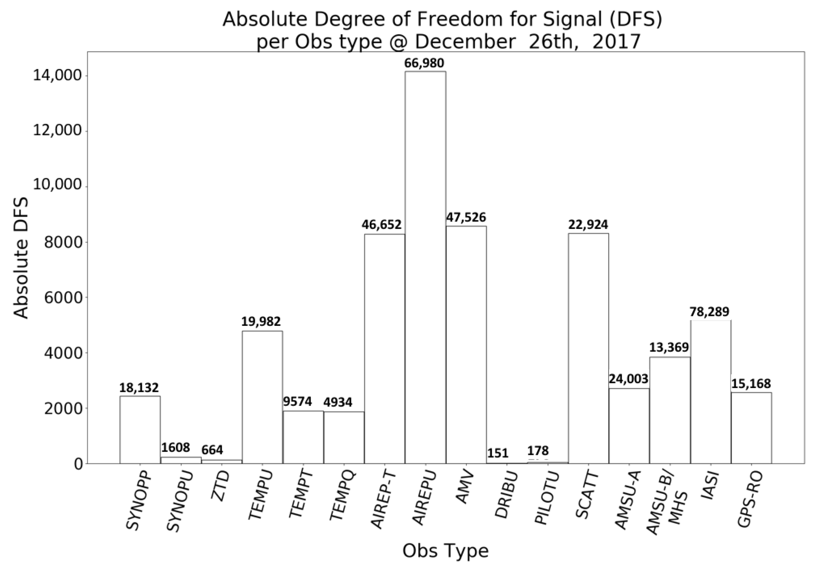
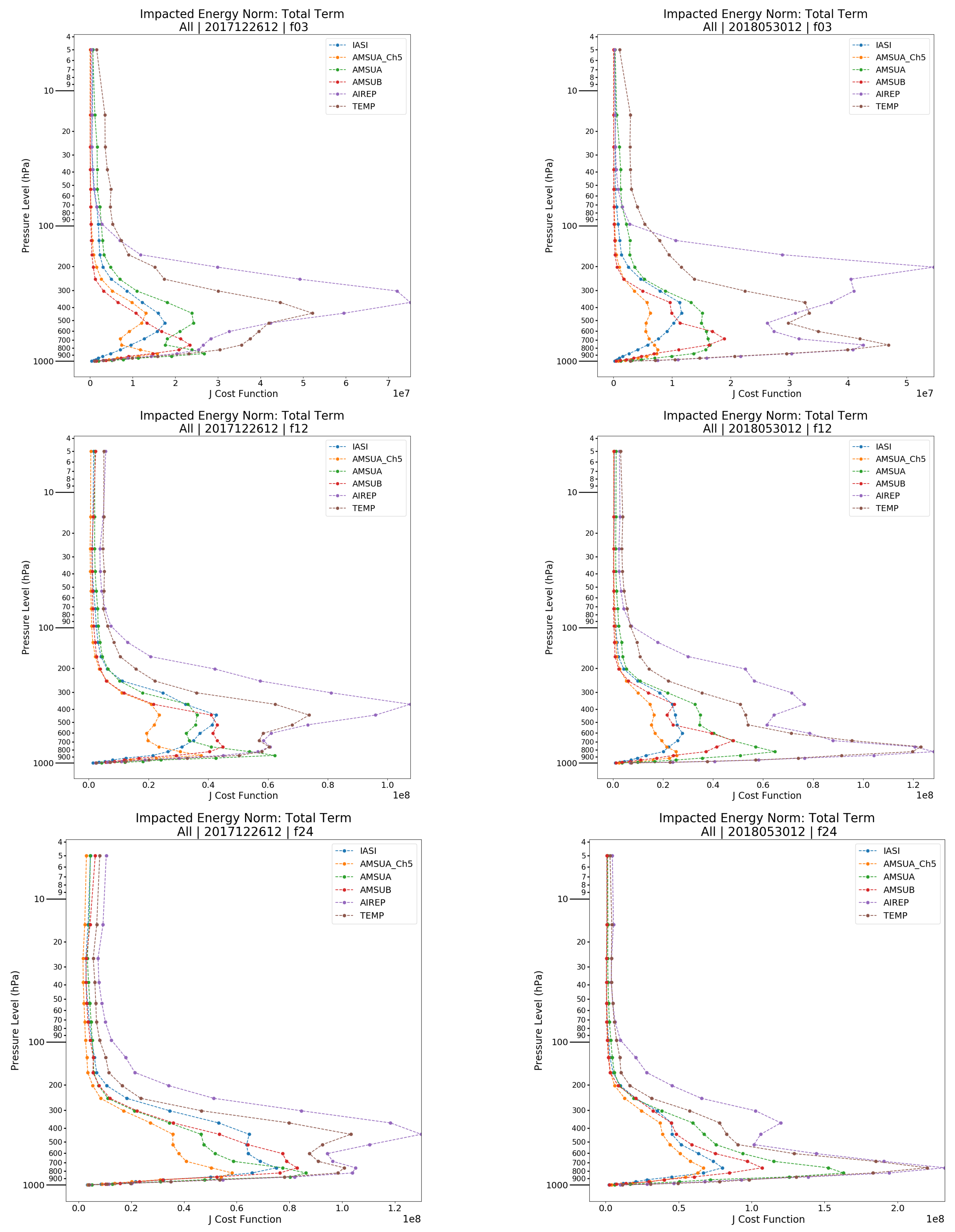
The relative impacts of the satellite radiance observations on the CERRA data assimilation and forecast systems were assessed using DFS and MTEN diagnostic metrics. The results indicate that the conventional observations had the strongest impact on both the analysis and forecasts. However, the difference in impact between the radiance and conventional observations is smaller for the short-range (12 and 24-h) forecasts. In other words, the impact of the radiance observation is more predominant on longer forecast lengths. Similar results have been observed in studies with a similar regional model setup [41].
The discussion in this paper focused mainly on the impact of radiance observations on geopotential height analyses and forecasts since it has the most distinguishable statistical significance of the impacts compared to that of the other verified variables. This means that less significant impacts of the satellite radiance observations on the other upper-air and surface variables were observed, but not discussed.
The impacts of the satellite radiance observations and their significance were demonstrated through examining the normalized mean RMSE difference of 21+ days OSEs during winter and summer periods. Overall, satellite radiance observations have a neutral impact on the analyses of geopotential height in the lower troposphere, while a slightly negative impact for the upper troposphere and in the stratosphere. Similar neutral impacts were also observed in 3-h forecasts and positive impacts on the 12 and 24-h forecasts (Figure 15 and Figure 16). The 6-h forecast at 18 UTC was problematic due to the observed large negative impact above 300 hPa. Further investigation was done to determine the cause of this significant negative impact. The preliminary findings suggest that AMSU-A and IASI have the greatest impact on geopotential, while a weaker impact was seen from AMUS-B/MHS. Additional OSEs were conducted for AMSU-A and IASI observations over land. The results showed that AMSU-A had a neutral impact on the analysis while reducing the errors up to 2.5% for the 3-h forecasts below 300 hPa. On the other hand, IASI observation over land generally increases the errors in the analysis, as well as in the 3 and 6-h forecasts. This can be caused by a lack of consideration of surface emissivity and skin temperature to appropriately assimilate IASI observations over land in the CERRA system. By rejecting this subset of observations, an improvement in the analysis and 3-h forecast accuracy was observed in the upper troposphere. Similar improvement was observed in the stratosphere for the 6-h forecasts from 18 UTC cycle
The Desroziers method applied to the satellite radiance first-guess and analysis departures and verification of OSEs against radiosonde observations that led to the discovery of the radiance assimilation settings in the CERRA system did not appropriately consider the possible observation error correlation for certain assimilated instruments channels. The inflation of observations errors and the increase in the thinning distance were tested in rudimentary verification experiments. The obtained results suggest that increasing the thinning distance (RMIND_RAD1C = 100 km and RFIND_RAD1C = 120 km) and rejecting IASI observations over land yield a considerable error reduction in the forecasts of geopotential heights. These findings are also reflected in a 21+ days OSE in the summer and winter periods, where the errors were reduced up to 2% for the analyses and 3-h forecasts. In addition, the large errors in the upper troposphere and in the stratosphere observed in the 6-h forecasts from 18 UTC were greatly reduced, although the error reduction in the lower troposphere was slightly diminished. Despite this fact, the tested configuration enhanced the CERRA system by improving the accuracy of the analyses and the 3-h forecasts, while keeping the positive impacts on the short-range forecasts (12 and 24 h).
Applying the modified configurations showed that the assimilation of radiance observations improves the accuracy of short range forecasts (12- and 24-h) of geopotential in the lower and mid-troposphere, while neutral to slightly positive impact was observed on the 3-h forecast. Neutral impact was also observed in the tropospheric levels of the analyses, while an increased error was detected for the stratosphere. The increase in error in the analysis, verified against the radiosonde observations does not necessarily indicate the analyses has deteriorated. It is more likely due to the fact that the assimilation of radiance observations causes such a balance between the control variables, which deviates from the observed radiosonde network. This balance seems to represent better the atmospheric state, since the issued forecasts (12 and 24 h) are of significantly better quality.
Overall, the assimilation of radiance observation provides a relatively small, but significant positive impact on the analysis and forecasts in reducing the normalized mean RMSE errors in geopotential heights. Given the short development period of the CERRA system and limited computational resources, it was not feasible to further enhance the assimilation of the radiance observations. The development of subsequent generations of the CERRA system can benefit from the results of this study and further continue the investigation of reducing the effect of high observation error correlations by combining the utilization of observation error inflation and observation thinning to preserve the small-scale information from observations, as discussed in [50].

Author Contributions

Conceptualization, Z.Q.W. and R.R.; methodology, Z.Q.W. and R.R.; validation, Z.Q.W. and R.R.; formal analysis, Z.Q.W. and R.R.; investigation, Z.Q.W. and R.R.; data curation, Z.Q.W. and R.R.; writing—original draft preparation, Z.Q.W.; writing—review and editing, R.R.; visualization, Z.Q.W. and R.R. All authors have read and agreed to the published version of the manuscript.

Funding

Copernicus Climate Change Services (C3S_322 Lot 1), Copernicus European Regional Reanalysis (CERRA) at https://climate.copernicus.eu/regional-reanalysis-europe.

Acknowledgments

The authors would like to thank the staff on the CERRA development team for the collaborative effort in developing the system and monitoring the production of the reanalysis dataset. This includes Adam El Said, Antoine Verrelle, Eric Bazile, Esbjörn Olsson, Lars Berggren, Martin Ridal, Michael Glinton, Semjon Schimanke, Susanna Hagelin, Susanna Hopsch Patrick Le Moigne, Paulo Medeiros and Per Dahlgren.

Conflicts of Interest

The authors declare no conflict of interest.

Abbreviations

The following abbreviations are used in this manuscript:
3D-VARThree-dimensional Variational Data Assimilation
AIREPAircraft Observations
ALADINAire Limitée Adaptation Dynamique Développement International
AMSU-AAdvanced Microwave Sounding Unit-A
AMSU-BAdvanced Microwave Sounding Unit-B
AMVAtmospheric Motion Vectors
AROMEApplication of Research to Operations at Mesoscale
ARPEGEAction de Recherche Petite Echelle Grande Echelle
ATOVSAdvanced TIROS Operational Vertical Sounder
BTBrightness Temperature
C3SCopernicus Climate Change Service
CERRACopernicus Regional Reanalysis for Europe
ECMWFEuropean Centre for Medium-Range Weather Forecasts
EDAEnsemble Data Assimilation
EFDEnsemble Flow Dependent
FGFirst-Guess
FMIFinnish Meteorological Institute
FP7Seventh Framework Programme
GPS-ROGPS Radio Occultation
ZTDZenith Total Delay
HIRLAMHigh-Resolution Limited Area Model
IASIInfrared Atmospheric Sounding Interferometer
IFSIntegrated Forecast System
IMOIcelandic Meteorological Office
IRInfrared
LAMLimited Area Model
MTENMoist Total Energy Norm
MHSMicrowave Humidity Sounder
MSUMicrowave Sounding Unit
NWPNumerical Weather Prediction
OIOptimal Interpolation
OMAObservation Minus the analysis
OMFObservation Minus the First-Guess
OSEObserving System Experiments
PILOTPilot Observation
RMSERoot Mean Square Error
SCATTScattomemter
SMHISwedish Meteorological and Hydrological Institute
SYNOPSurface Synoptic Observations
TEMPRadiosonde Sounding Observations
UERRAUncertainty in Ensemble of Regional Reanalysis
VARBCVariational Bias Correction

References

  1. Kalnay, E.; Kanamitsu, M.; Kistler, R.; Collins, W.; Deaven, D.; Gandin, L.; Iredell, M.; Saha, S.; White, G.; Woollen, J.; et al. The NCEP/NCAR 40-year reanalysis project. Bull. Am. Meteorol. Soc. 1996, 77, 437–472. [Google Scholar] [CrossRef] [Green Version]
  2. Harada, Y.; Kamahori, H.; Kobayashi, C.; Endo, H.; Kobayashi, S.; Ota, Y.; Onoda, H.; Onogi, K.; Miyaoka, K.; Takahashi, K. The JRA-55 Reanalysis: Representation of atmospheric circulation and climate variability. J. Meteorol. Soc. Jpn. Ser. II 2016, 94, 269–302. [Google Scholar] [CrossRef] [Green Version]
  3. Hersbach, H.; Bell, B.; Berrisford, P.; Hirahara, S.; Horányi, A.; Muñoz-Sabater, J.; Nicolas, J.; Peubey, C.; Radu, R.; Schepers, D.; et al. The ERA5 global reanalysis. Q. J. R. Meteorol. Soc. 2020, 146, 1999–2049. [Google Scholar] [CrossRef]
  4. Ulazia Manterola, A.; Sáenz Aguirre, J.; Ibarra Berastegi, G.; González Rojí, S.J.; Carreno Madinabeitia, S. Global estimations of wind energy potential considering seasonal air density changes. Energy 2019, 187, 115938. [Google Scholar] [CrossRef]
  5. Dee, D.P.; Uppala, S.M.; Simmons, A.; Berrisford, P.; Poli, P.; Kobayashi, S.; Andrae, U.; Balmaseda, M.; Balsamo, G.; Bauer, D.P.; et al. The ERA-Interim reanalysis: Configuration and performance of the data assimilation system. Q. J. R. Meteorol. Soc. 2011, 137, 553–597. [Google Scholar] [CrossRef]
  6. Ridal, M.; Esbjörn, O.; Unden, P.; Zimmermann, K.; Ohlsson, A. Uncertainties in Ensembles of Regional Re-Analyses: HARMONIE reanalysis report of results and dataset. In Project Deliverable Report D2.7; 2017; Available online: https://www.uerra.eu/component/dpattachments/?task=attachment.download&id=297 (accessed on 24 January 2021).
  7. Termonia, P.; Fischer, C.; Bazile, E.; Bouyssel, F.; Brožková, R.; Bénard, P.; Bochenek, B.; Degrauwe, D.; Derková, M.; El Khatib, R.; et al. The ALADIN System and its canonical model configurations AROME CY41T1 and ALARO CY40T1. Geosci. Model Dev. 2018, 11, 257–281. [Google Scholar] [CrossRef] [Green Version]
  8. Fischer, C.; Montmerle, T.; Berre, L.; Auger, L.; Ştefănescu, S.E. An overview of the variational assimilation in the ALADIN/France numerical weather-prediction system. Q. J. R. Meteorol. Soc. J. Atmos. Sci. Appl. Meteorol. Phys. Oceanogr. 2005, 131, 3477–3492. [Google Scholar] [CrossRef]
  9. Giard, D.; Bazile, E. Implementation of a new assimilation scheme for soil and surface variables in a global NWP model. Mon. Weather Rev. 2000, 128, 997–1015. [Google Scholar] [CrossRef]
  10. El-Said, A. The HARMONIE-ALADIN EDA system Estimation of uncertainties in the model system Brief overview and validation. In CERRA Deliverable Report D322_Lot1.1.1.7; 2020; Available online: https://silense.eu/content/deliverable-report-d-332-design-simulation-environment (accessed on 24 January 2021).
  11. Brousseau, P.; Berre, L.; Bouttier, F.; Desroziers, G. Flow-dependent background-error covariances for a convective-scale data assimilation system. Q. J. R. Meteorol. Soc. 2012, 138, 310–322. [Google Scholar] [CrossRef]
  12. Buehner, M. Ensemble-derived stationary and flow-dependent background-error covariances: Evaluation in a quasi-operational NWP setting. Q. J. R. Meteorol. Soc. J. Atmos. Sci. Appl. Meteorol. Phys. Oceanogr. 2005, 131, 1013–1043. [Google Scholar] [CrossRef]
  13. Derber, J.C.; Wu, W.S. The use of TOVS cloud-cleared radiances in the NCEP SSI analysis system. Mon. Weather Rev. 1998, 126, 2287–2299. [Google Scholar] [CrossRef]
  14. Kazumori, M. Satellite radiance assimilation in the JMA operational mesoscale 4DVAR system. Mon. Weather Rev. 2014, 142, 1361–1381. [Google Scholar] [CrossRef]
  15. McNally, A.P.; Derber, J.; Wu, W.; Katz, B. The use of TOVS level-1b radiances in the NCEP SSI analysis system. Q. J. R. Meteorol. Soc. 2000, 126, 689–724. [Google Scholar] [CrossRef]
  16. Randriamampianina, R. Impact of high resolution satellite observations in the ALADIN/HU model. Q. J. Hung. Meteorol. Serv. 2006, 110, 329–347. [Google Scholar]
  17. Randriamampianina, R.; Schyberg, H.; Mile, M. Observing system experiments with an Arctic mesoscale numerical weather prediction model. Remote Sens. 2019, 11, 981. [Google Scholar] [CrossRef] [Green Version]
  18. Auligné, T.; McNally, A.; Dee, D. Adaptive bias correction for satellite data in a numerical weather prediction system. Q. J. R. Meteorol. Soc. J. Atmos. Sci. Appl. Meteorol. Phys. Oceanogr. 2007, 133, 631–642. [Google Scholar] [CrossRef]
  19. Dee, D.P.; Uppala, S. Variational bias correction of satellite radiance data in the ERA-Interim reanalysis. Q. J. R. Meteorol. Soc. J. Atmos. Sci. Appl. Meteorol. Phys. Oceanogr. 2009, 135, 1830–1841. [Google Scholar] [CrossRef]
  20. Randriamampianina, R.; Iversen, T.; Storto, A. Exploring the assimilation of IASI radiances in forecasting polar lows. Q. J. R. Meteorol. Soc. 2011, 137, 1700–1715. [Google Scholar] [CrossRef]
  21. Desroziers, G.; Berre, L.; Chapnik, B.; Poli, P. Diagnosis of observation, background and analysis-error statistics in observation space. Q. J. R. Meteorol. Soc. J. Atmos. Sci. Appl. Meteorol. Phys. Oceanogr. 2005, 131, 3385–3396. [Google Scholar] [CrossRef]
  22. Bormann, N.; Bauer, P. Estimates of spatial and interchannel observation-error characteristics for current sounder radiances for numerical weather prediction. I: Methods and application to ATOVS data. Q. J. R. Meteorol. Soc. 2010, 136, 1036–1050. [Google Scholar] [CrossRef]
  23. Liu, Z.Q.; Rabier, F. The potential of high-density observations for numerical weather prediction: A study with simulated observations. Q. J. R. Meteorol. Soc. J. Atmos. Sci. Appl. Meteorol. Phys. Oceanogr. 2003, 129, 3013–3035. [Google Scholar] [CrossRef]
  24. Bengtsson, L.; Andrae, U.; Aspelien, T.; Batrak, Y.; Calvo, J.; de Rooy, W.; Gleeson, E.; Hansen-Sass, B.; Homleid, M.; Hortal, M.; et al. The HARMONIE–AROME model configuration in the ALADIN–HIRLAM NWP system. Mon. Weather. Rev. 2017, 145, 1919–1935. [Google Scholar] [CrossRef]
  25. Migliorini, S.; Candy, B. All-sky satellite data assimilation of microwave temperature sounding channels at the Met Office. Q. J. R. Meteorol. Soc. 2019, 145, 867–883. [Google Scholar] [CrossRef]
  26. McNally, A.; Watts, P. A cloud detection algorithm for high-spectral-resolution infrared sounders. Q. J. R. Meteorol. Soc. J. Atmos. Sci. Appl. Meteorol. Phys. Oceanogr. 2003, 129, 3411–3423. [Google Scholar] [CrossRef]
  27. Krzeminski1, B.; Bormann, N.; Karbou, F.; Bauer, P. Towards a better use of AMSU over land at ECMWF. In Proceedings of the ITSC-XVI, Angra dos Reis, Brazil, 7–13 May 2008. [Google Scholar]
  28. Geer, A.J.; Lonitz, K.; Weston, P.; Kazumori, M.; Okamoto, K.; Zhu, Y.; Liu, E.H.; Collard, A.; Bell, W.; Migliorini, S.; et al. All-sky satellite data assimilation at operational weather forecasting centres. Q. J. R. Meteorol. Soc. 2018, 144, 1191–1217. [Google Scholar] [CrossRef]
  29. Karbou, F.; Gérard, É.; Rabier, F. Microwave land emissivity and skin temperature for amsu-A and-B assimilation over land. Q. J. R. Meteorol. Soc. J. Atmos. Sci. Appl. Meteorol. Phys. Oceanogr. 2006, 132, 2333–2355. [Google Scholar] [CrossRef] [Green Version]
  30. Karbou, F.; Gérard, E.; Rabier, F. Global 4DVAR assimilation and forecast experiments using AMSU observations over land. Part I: Impacts of various land surface emissivity parameterizations. Weather Forecast. 2010, 25, 5–19. [Google Scholar] [CrossRef]
  31. Deblonde, G.; English, S. Evaluation of the FASTEM-2 fast microwave oceanic surface emissivity model. In Proceedings of the 11th International ATOVS Study Conference, Budapest, Hungary, 20–26 September 2000; pp. 67–78. [Google Scholar]
  32. Prigent, C.; Aires, F.; Wang, D.; Fox, S.; Harlow, C. Sea-surface emissivity parametrization from microwaves to millimetre waves. Q. J. R. Meteorol. Soc. 2017, 143, 596–605. [Google Scholar] [CrossRef]
  33. Prigent, C.; Chevallier, F.; Karbou, F.; Bauer, P.; Kelly, G. AMSU-A land surface emissivity estimation for numerical weather prediction assimilation schemes. J. Appl. Meteorol. 2005, 44, 416–426. [Google Scholar] [CrossRef] [Green Version]
  34. Saunders, R.; Hocking, J.; Turner, E.; Rayer, P.; Rundle, D.; Brunel, P.; Vidot, J.; Roquet, P.; Matricardi, M.; Geer, A.; et al. An update on the RTTOV fast radiative transfer model (currently at version 12). Geosci. Model Dev. 2018, 11, 2717–2737. [Google Scholar] [CrossRef] [Green Version]
  35. Dando, M.; Thorpe, A.; Eyre, J. The optimal density of atmospheric sounder observations in the Met Office NWP system. Q. J. R. Meteorol. Soc. J. Atmos. Sci. Appl. Meteorol. Phys. Oceanogr. 2007, 133, 1933–1943. [Google Scholar] [CrossRef]
  36. Lindskog, M. ATOVS Processing and Usage in the HARMONIE Reference System. HIRLAM Newsl. 2010, 59, 33–43. [Google Scholar]
  37. Dee, D.P. Variational bias correction of radiance data in the ECMWF system. In Proceedings of the ECMWF Workshop on Assimilation of High Spectral Resolution Sounders in NWP, Reading, UK, 28 June–1 July 2004; Volume 28, pp. 97–112. [Google Scholar]
  38. Harris, B.; Kelly, G. A satellite radiance-bias correction scheme for data assimilation. Q. J. R. Meteorol. Soc. 2001, 127, 1453–1468. [Google Scholar] [CrossRef]
  39. Hilton, F.; Atkinson, N.; English, S.; Eyre, J. Assimilation of IASI at the Met Office and assessment of its impact through observing system experiments. Q. J. R. Meteorol. Soc. J. Atmos. Sci. Appl. Meteorol. Phys. Oceanogr. 2009, 135, 495–505. [Google Scholar] [CrossRef]
  40. Chapnik, B.; Desroziers, G.; Rabier, F.; Talagrand, O. Diagnosis and tuning of observational error in a quasi-operational data assimilation setting. Q. J. R. Meteorol. Soc. J. Atmos. Sci. Appl. Meteorol. Phys. Oceanogr. 2006, 132, 543–565. [Google Scholar] [CrossRef]
  41. Storto, A.; Randriamampianina, R. The relative impact of meteorological observations in the Norwegian regional model as determined using an energy norm-based approach. Atmos. Sci. Lett. 2010, 11, 51–58. [Google Scholar] [CrossRef]
  42. Rabier, F.; Fourrié, N.; Chafäi, D.; Prunet, P. Channel selection methods for infrared atmospheric sounding interferometer radiances. Q. J. R. Meteorol. Soc. J. Atmos. Sci. Appl. Meteorol. Phys. Oceanogr. 2002, 128, 1011–1027. [Google Scholar] [CrossRef] [Green Version]
  43. Cardinali, C.; Pezzulli, S.; Andersson, E. Influence-matrix diagnostic of a data assimilation system. Q. J. R. Meteorol. Soc. J. Atmos. Sci. Appl. Meteorol. Phys. Oceanogr. 2004, 130, 2767–2786. [Google Scholar] [CrossRef]
  44. Ehrendorfer, M.; Errico, R.M.; Raeder, K.D. Singular-vector perturbation growth in a primitive equation model with moist physics. J. Atmos. Sci. 1999, 56, 1627–1648. [Google Scholar] [CrossRef] [Green Version]
  45. Gelaro, R.; Zhu, Y. Examination of observation impacts derived from observing system experiments (OSEs) and adjoint models. Tellus A Dyn. Meteorol. Oceanogr. 2009, 61, 179–193. [Google Scholar] [CrossRef]
  46. Bauer, P.; Radnóti, G.; Healy, S.; Cardinali, C. GNSS radio occultation constellation observing system experiments. Mon. Weather Rev. 2014, 142, 555–572. [Google Scholar] [CrossRef]
  47. Lawrence, H.; Bormann, N.; Sandu, I.; Day, J.; Farnan, J.; Bauer, P. Use and impact of Arctic observations in the ECMWF Numerical Weather Prediction system. Q. J. R. Meteorol. Soc. 2019, 145, 3432–3454. [Google Scholar] [CrossRef] [Green Version]
  48. Geer, A.J. Significance of changes in medium-range forecast scores. Tellus A Dyn. Meteorol. Oceanogr. 2016, 68, 30229. [Google Scholar] [CrossRef] [Green Version]
  49. Bormann, N.; Bauer, P. Estimates of spatial and interchannel observation-error characteristics for current sounder radiances for numerical weather prediction. II: Application to AIRS and IASI data. Q. J. R. Meteorol. Soc. 2010, 136, 1051–1063. [Google Scholar] [CrossRef]
  50. Bédard, J.; Buehner, M. A practical assimilation approach to extract smaller-scale information from observations with spatially correlated errors: An idealized study. Q. J. R. Meteorol. Soc. 2020, 146, 468–482. [Google Scholar] [CrossRef] [Green Version]
Figure 1. The domain of the Copernicus European Regional Reanalysis (CERRA) system represented by the highlighted region in blue shading.
Remotesensing 13 00426 g001
Figure 2. A summary of the coupled Ensemble Data Assimilation (EDA) and deterministic system represented by the orange and blue colour shading, respectively. The B-Matrix is updated using the forecast differences from the 10 ensemble members. The three-dimensional variational (3D-VAR) from the deterministic system uses the updated B-Matrix to assimilate recent observations and compute the analysis. The forecasts are initialized using the analyses and integrated in time using the LBCs, while the 3-h forecasts are used as the first guess or background for the assimilation in the following cycle.
Remotesensing 13 00426 g002
Figure 3. The normalized weighting function for all assimilated IASI channels.
Remotesensing 13 00426 g003
Figure 4. A workflow diagram of the two-step data assimilation approach used to spin up the VARBC coefficients in the CERRA system.
Remotesensing 13 00426 g004
Figure 5. The (left,right) plot depicts the time evolution of the at 9 UTC assimilation cycle for IASI channel 239 on MetOp-B (AMSUA channel 6 on MetOp-A) during a 47-day (30 days) VARBC spin-up period. The predictors used are shown at the bottom of the plots.
Remotesensing 13 00426 g005
Figure 6. The (top-left) plot (top-right) illustrates the evolution of biases at 9 UTC assimilation for IASI channel 239 on MetOp-B (AMSU-A channel 6 on MetOp-A) during a 47-day (30 days) VARBC spin-up period. The dashed line represents the non-corrected observation minus first-guess (non-cor OMF) bias, while the solid line depicts the corrected observation minus first-guess (OMF) bias. The bold solid line shows the corrected observation minus analysis (OMA) bias. The green (blue) line shows the biases for observations over land (sea). The bottom plots illustrate the number of observations over land (sea) shown by the green (blue) bar.
Remotesensing 13 00426 g006
Figure 7. The time-series of the biases at 9 UTC assimilation time for IASI channel 296 on MetOp-B during a 23-day active assimilation experiment from the full CERRA system (top-left). The number of observations over land (sea) shown by the green (blue) bar (bottom-left). The time-series of bias correction predictor coefficients (right).
Remotesensing 13 00426 g007
Figure 8. The left plot shows the biases of the 55 IASI channels that are actively assimilated in the full operational CERRA system. The non-corrected OMF (dashed line) bias, corrected OMF bias (solid line) and OMA bias (bolded line). The green (blue) lines represent the respective biases for observations over land (sea). The right plot shows the number of observations over land (green) and sea (blue) for each channel.
Remotesensing 13 00426 g008
Figure 9. The absolute DFS computed from all assimilation times on 26 December 2017. All observations that are assimilated in the CERRA system were examined, including geopotential height (SYNOP Z) and wind components (SYNOP U) measurements from land surface stations; drift buoys (DRIBU); wind components (TEMP U), temperature (TEMP T) and specific humidity (TEMP Q) measurements from radiosonde; wind components (AIREP U) and temperature (AIREP T) measurements from aircraft observations; wind components from pilots or PIREP (PILOT U); zenith total delay (ZTD); GNSS Radio-Occultation (GPS-RO); Atmospheric Motion Vector (AMV); Scattometer (SCATT); Advance Microwave Sounding Unit-A (AMSU-A), Advanced Microwave Sounding Unit-B and Microwave Humidity Sounder (AMSU-B); and Infrared Atmospheric Sounding Interferometer (IASI). The numerical values above the bar plots represent the number of each observation type.
Remotesensing 13 00426 g009
Figure 10. Vertical profiles of the loss of moist total energy norm (MTEN) in CERRA forecasts when removing subsets of observation from the assimilation system, including aircraft (AIREP), radiosonde (TEMP), IASI, AMSU-B/MHS (AMSU-B), AMSU-A (AMSUA) and only channel 5 from AMSU-A (AMSUA_Ch5) observations. The first and second columns show the results for forecasts initialized from 12 UTC on 26 January 2018 and 30 May 2018, respectively. The 3 (f03), 12 (f12) and 24 (f24) hour forecasts are shown in the first, second and third rows, respectively.
Remotesensing 13 00426 g010
Figure 11. The vertical profile of the normalized by the mean scores, Root Mean Square Error (RMSE) difference at 90% confidence for the geopotential height (in meter) between the control experiment (“AllSat”) and the individual experiments (“NoAMSUA” (blue), “NoIASI(Land)” (orange) or “NoRad” (green)). The AllSat experiment assimilates all observations; the “NoAMSUA” experiment assimilates all observations, except for AMSU-A; “NoIASI(Land)” experiment assimilates all observations, except for IASI observations over land; “NoRad” does not assimilate any radiance observations. The computed statistics are valid for the winter case, spanning from 23 December 2017 to 16 January 2018. Each subplot depicts the comparison at a specific analysis (F00) or forecast lengths (F03) that is initialized at a particular assimilation time.
Remotesensing 13 00426 g011
Figure 12. The same as Figure 11, but for the summer case and different forecast lengths, spanning from 28 May to 19 June 2018.
Remotesensing 13 00426 g012
Figure 13. The observation error correlation with respect to the spatial separation distance of pairing observations for AMSU-A channel 5–9 ( 53.596 ± 0.115 57.290 GHz), computed from the Desroziers diagnostic (left plot). The number of observation samplings for the respective channels (right plot).
Remotesensing 13 00426 g013
Figure 14. A vertical profile of Root Mean Square Error (RMSE) difference of 6-h forecast geopotential height between the control experiment (Thin_60_80 km) and the four impact experiments. The 6-h geopotential height forecasts, initialized at 18 UTC on 30 May 2018 were verified against radiosonde observations. Table 6 summarizes the configuration of the five experiments that were examined in this comparison.
Remotesensing 13 00426 g014
Figure 15. The vertical profile of the normalized by the mean scores Root Mean Square Error (RMSE) difference for geopotential height (at 90% confidence) between the four impact experiments (“AllSat”, “NoIASI(Land)” or “Thin(100–120 km)_noIASI(Land)”) minus the control experiment (“NoRad”). The control experiment assimilates all observations, except the radiance observations; “AllSat” experiment assimilates all observations; “NoIASI(Land)” experiment assimilates all observations, except the IASI observations over land; “Thin(100–120 km)_noIASI(Land)” experiment assimilates all observations, except the IASI observations over land and have an increased thinning distance at RMIND_RAD1C = 100 km and RFIND_RAD1C = 120 km for all radiance observations. Therefore, the performance of the three impact experiments are relative to the control experiment. The computed statistics are valid for the winter case, spanning from 23 December 2017 to 16 January 2018. Each subplot depicts the comparison at a specific analysis (F00) or forecast lengths (F03, F12) that is initialized at a particular assimilation cycle.
Remotesensing 13 00426 g015
Figure 16. Same as Figure 15 but for the summer case, spanning from 28 May to 19 June 2018.
Remotesensing 13 00426 g016
Table 1. Summary of the non-satellite observations assimilated in the CERRA system. The sources of the observations are listed. Note that MARS represents the European Centre for Medium-Range Weather Forecast’s (ECMWF) Meteorological Archival and Retrieval System.
TypeSource
Conventional (radiosonde, aircrafts, ships, buoys and surface observations)MARS
Local ObservationDMI, SMHI, MET Norway, FMI, IMO, Météo France
Table 2. Summary of the satellite observations assimilated in the CERRA system. The satellite platforms of each instrument and the source of the observation datasets are listed. Note that MARS represents ECMWF’s Meteorological Archival and Retrieval System, and ECFS is ECMWF’s file storage system.
InstrumentSatellitesSources
Advanced Microwave Sounding Unit-A (AMSU-A)NOAA-15,16,18,19, MetOp-A,B,CMARS Archive
Advanced Microwave Sounding Unit-B (AMSU-B) and Microwave Humidity Sensor (MHS)NOAA-16,17,18,19 MetOp-A,B,CMARS Archive
Microwave Sounding Unit (MSU)NOAA-6,7,8,9,10,11,12,14MARS Archive
Infrared Atmospheric Sounding Interferometer (IASI)MetOp-A,B,CEUMETCAST Dataset and MARS Archive
Atmospheric Motion Vectors (AMV)NOAA, MetOp, METEOSATMARS Archive
ScatterometerNSCAT-ERS2, Seawinds-QuickSCAT, OceanSat2-OceanSCAT, Metop-A,B,C-ASCATEUMETSAT Data Center
GPS Radio Occultation (GPS-RO)Metop, COSMIC, CHAMP, GRACEReprocessed Climate Data Records
Ground-Based GNSS-ZTD (GPS-ZTD)GPS and GLONASSEPN EUREF, EUREF GNSS
Table 3. A summary of the instruments, satellite platforms, channels and its respective frequencies (microwave instruments) or wavenumber (IR instrument) that are assimilated within the CERRA reanalysis period. Infrared Atmospheric Sounding Interferometer (IASI) channels 333 and 352 are later rejected, which will be explained in Section 5.
InstrumentsSatellite PlatformChannelsFrequency (GHz)-Microwave
Wavenumber (cm 1 )-IR
MSUNOAA-6, 7, 9, 10, 11, 12, 142,3,453.74, 54.96, 57.95
AMSU-ANOAA-15, 16, 18, 19, Metop-A, B, C5,6,7,8,953.596 ± 0.115, 54.40, 54.94, 55.50, 57.290
AMSU-BNOAA-16, 17, 183,4,5183.31 ± 1.0, 183.31 ± 3.0, 190.311
MHSNOAA-19 METOP-A, B, C3,4,5183.31 ± 1.0, 183.31 ± 3.0, 190.311
IASIMETOP-A, B, C CO 2 Absorption Band: 38, 51, 63, 85, 104, 109, 167, 173, 180, 185, 193, 199, 205, 207, 212, 224, 230, 236, 239, 242, 243, 249, 296, 333*, 337, 345, 352*, 386, 389, 432
H 2 O Absorption Band: 2701, 2819, 2910, 2919, 2991, 2993, 3002, 3008, 3014, 3098, 3207, 3228, 3281, 3309, 3322, 3438, 3442, 3484, 3491, 3499, 3506, 3575, 3582, 3658, 4032
CO 2 Absorption Band: 654.25, 657.50, 660.50, 666.00, 670.75, 672.00, 686.50, 688.00, 689.75, 691.00, 693.00, 694.50, 696.00, 696.50, 697.75, 700.75, 702.25, 703.75, 704.50, 705.25, 705.50, 707.00, 718.75, 728.00, 729.00, 731.00, 732.75, 741.25, 742.00, 752.75
H 2 O Absorption Band: 1320.00, 1349.50, 1372.25, 1374.50, 1392.50, 1393.00, 1395.25, 1396.75, 1398.25, 1419.25, 1446.50, 1451.75, 1465.00, 1472.00, 1475.25, 1504.25, 1505.25, 1515.75, 1517.50, 1519.50, 1521.25, 1538.50, 1540.25, 1559.25, 1652.75
Table 4. The thinning distance parameters for the assimilation of the radiance observations used in the CERRA system.
InstrumentRMIND_RAD1C (km)RFIND_RAD1C (km)
AMSU-A6080
AMSU-B4080
MHS4080
IASI6080
Table 5. The relevant variational bias correction (VARBC) bias correction predictors used in the HARMONIE numerical weather prediction (NWP) system.
PredictorExplanation
p01 (Constant)
p11000–300 hPa thickness
p2200–50 hPa thickness
p3T_skin
p4total column water
p510–1 hPa thickness
p650–5 hPa thickness
p7surface wind speed
p8nadir viewing angle
p9nadir view angle **2
p10nadir view angle **3
p15nadir viewing angle (Land)
p16nadir view angle **2 (Land)
p17nadir view angle **3 (Land)
Table 6. A summary of the experiments with different thinning distance parameters, observation error inflation and observation rejection settings. RMIND_RAD1C limits the minimum horizontal distance between a pair of observations, while RFIND_RAD1C is the average horizontal distance between a pair of observations after thinning.
ExperimentsRMIND_RAD1C (km)RFIND_RAD1C (km)Rejected IASI Channels
Thin_60_80 km (Control Experiment)Adopted from Table 3Adopted from Table 3No
80_100 km + Blk80 km100 km104, 180, 2991, 3098, 3309, 3506
100_120 km + Blk100 km120 km104, 180, 2991, 3098, 3309, 3506
110_130 km + Blk110 km130 km104, 180, 2991, 3098, 3309, 3506
AMSUA Sigma_O x2Inflate observation errors for AMSUA radiance observation by 2 factors
Publisher’s Note: MDPI stays neutral with regard to jurisdictional claims in published maps and institutional affiliations.

