Article

NDVI as a Proxy for Estimating Sedimentation and Vegetation Spread in Artificial Lakes—Monitoring of Spatial and Temporal Changes by Using Satellite Images Overarching Three Decades

1
Department of Physical Geography and Geoinformation Systems, University of Debrecen, Egyetem tér 1., 4032 Debrecen, Hungary
2
MTA-ÖK Lendület Seed Ecology Research Group, Institute of Ecology and Botany, Centre for Ecological Research, Alkotmány u. 2-4., 2163 Vácrátót, Hungary
3
Department of Regional Water Management, National University of Public Service Faculty of Water Sciences, Bajcsy-Zsilinszky 12-14., 6500 Baja, Hungary
4
Department of Evolutionary Zoology, University of Debrecen, Egyetem tér 1., 4032 Debrecen, Hungary
*
Author to whom correspondence should be addressed.
Remote Sens. 2020, 12(9), 1468; https://doi.org/10.3390/rs12091468
Submission received: 29 March 2020 / Revised: 29 April 2020 / Accepted: 3 May 2020 / Published: 6 May 2020

Abstract

:
Observing wetland areas and monitoring changes are crucial to understand hydrological and ecological processes. Sedimentation-induced vegetation spread is a typical process in the succession of lakes endangering these habitats. We aimed to survey the tendencies of vegetation spread of a Hungarian lake using satellite images, and to develop a method to identify the areas of risk. Accordingly, we performed a 33-year long vegetation spread monitoring survey. We used the Normalized Difference Vegetation Index (NDVI) and the Modified Normalized Difference Water Index (MNDWI) to assess vegetation and open water characteristics of the basins. We used these spectral indices to evaluate sedimentation risk of water basins combined with the fact that the most abundant plant species of the basins was the water caltrop (Trapa natans) indicating shallow water. We proposed a 12-scale Level of Sedimentation Risk Index (LoSRI) composed from vegetation cover data derived from satellite images to determine sedimentation risk within any given water basin. We validated our results with average water basin water depth values, which showed an r = 0.6 (p < 0.05) correlation. We also pointed on the most endangered locations of these sedimentation-threatened areas, which can provide crucial information for management planning of water directorates and management organizations.

Graphical Abstract

1. Introduction

Remotely sensed (RS) images provide efficient tools for rapid data collection, can be deployed across extensive areas, and can also be effectively used to monitor changes in land cover and vegetation [1,2,3,4,5]. Satellites produce consistent data over long periods of time, e.g., Landsat and Satellite Pour l’Observation de la Terre (SPOT) [6,7,8]. The revisiting time of Landsat is 16 days, while Sentinel-2A and 2B together ensure 5 days of revisiting time; furthermore, a combination of Landsat and Sentinel data is possible and can be used in time series depending on the cloud cover [9,10]. Moderate Resolution Imaging Spectroradiometer (MODIS) or Planet Labs products provide daily acquisition [11,12,13]. Increased volumes, quality, and data coverage allow us to develop a better understanding of the natural and human factors that might affect land cover dynamics [14,15]. Although global-scale observations provide valuable results on land cover dynamics, studies specific to sites that have unique thematic focus will also be essential, if the aim is to support spatial planners, land managers, authorities, and decision makers.
Lakes and wetlands serve as important habitats for conservation. They have a considerable role in biodiversity conservation and also provide a huge variety of ecosystem services for all of society [16,17,18]. Because of huge losses over past centuries, as well as the sensitivity of these sites to eutrophication, and changes in land use and climate, wetlands are amongst the most endangered habitats globally. In addition to monitoring changes in their species composition, up-to-date records of land cover changes, as well as water quality and quantity (e.g., due to evaporation, precipitation, sedimentation, agricultural pollution, or tourism) are also essential for their effective conservation [19,20,21,22,23]. Attributes of a particular water basin can considerably influence its conservation potential and responses for disturbances; accordingly, large and deep basins, small and shallow basins, or oxbows all behave differently and have unique characteristics.
Lakes in Hungary are under threat for several reasons. On the one hand, aridity rates are increasing due to global warming [24,25], and a large number of smaller lakes suffer from scarce water supply and even can run dry at the end of the summer [26]. Although larger lakes can buffer the negative effects related to the arid climate, other factors also threaten these habitats, including the infiltration of nutrients and pollutants. Depending on the available nutrient surplus, lake succession and the spread of vegetation can accelerate eutrophication [27,28]; such a situation can be observed at Lake Fertő and Lake Kis-Balaton, which are already in a eutrophic state [29].
Deposited sediments can be the source of several problems in water management, including aggradation of floodplains [30,31] and accelerated sedimentation of lakes [32]. Monitoring lake sedimentation can be performed in several ways: analyzing sediment cores using radionuclides, heavy metals [33], or bioindicators [34,35]. These investigations provide valuable information on sedimentation but lack the spatial characteristic; only some points are sampled and the results are extrapolated. A direct spatial method involves mapping the bottom of lakes, which can be conducted using probe rods [36], sonar [37], or bathymetric LiDAR (Light Detection and Ranging) [38]. However, all these methods have limitations. Probe rod-based assessments are labor-intensive, and the number and distribution of surveyed points are related to the level of elaboration of the resulting map. Sonar is an efficient tool, but, together with the probe rod, its limitation is the approachability of lakesides (especially where water is shallow, i.e., <0.5 m, and the vegetation is dense); furthermore, sonar works well in deeper water. Bathymetric LiDAR can be used only when the water body’s turbidity is low and there is no vegetation cover, otherwise, emitted beams are adsorbed by suspended particles and are not reflected; thus, there is no recorded echo or the echo is due to vegetation. The common limitation of all techniques is uncertainty despite the high level of expenditure involved; furthermore, if the desired outcome is monitoring, assessment should be repeated regularly. A possible solution can be the application of optical remote sensing.
Satellite-based remote sensing using freely available data (Landsat, Sentinel) can be used to trace several fields of land cover change [39,40]. In addition to the original bands of the satellites, the use of spectral indices could enable more efficient monitoring [41,42,43]. Although spectral indices are well-known and have been widely utilized since the 1970s, and can help to reveal changes in open water area fluctuation, as well as the characteristics of water and vegetation, comprehensive long-term studies have so far not been reported for the Lake Tisza area. Moreover, such studies in general are scarce considering the large lakes of the world. In previous research, long-term lake monitoring has been achieved using satellite images, but the main goal of these projects was to evaluate the water level of Lake Victoria [44] and as the drought tendencies of a basin Salt Lake in Turkey [45]. Studies using MODIS products usually have relatively low resolution (250 or 500 m [46,47]) or range across shorter time periods using extremely high-resolution images [48]. Although Lake Tisza is endangered by the large amount of sediment carried by the Tisza River, there has been no comprehensive investigation to identify the most endangered areas. Furthermore, no previous studies have emphasized the dynamics of vegetation at the water surface over long time periods in the Lake Tisza area; nevertheless, vegetation spread can be a good indicator. We therefore conducted a long-term analysis using spectral indices (the Normalized Difference Vegetation Index (NDVI) and the Modified Normalized Difference Water Index (MNDWI)) sourced from RS Landsat data.
Lake Tisza (Figure 1) is an artificial water body in Hungary. The water level of the lake is regulated, and sedimentation and vegetation spread represent a continuous issue: differences in vegetation coverage and water depth are seen at more-or-less the same water level. The aims of this research were to reveal: (i) whether there any temporal trends in the spread of aquatic vegetation; and (ii) which water basin types exhibit the fastest succession rate. We also aimed to develop a method to determine the risk of vegetation spread by water basins of the lake using satellite images.

2. Materials and Methods
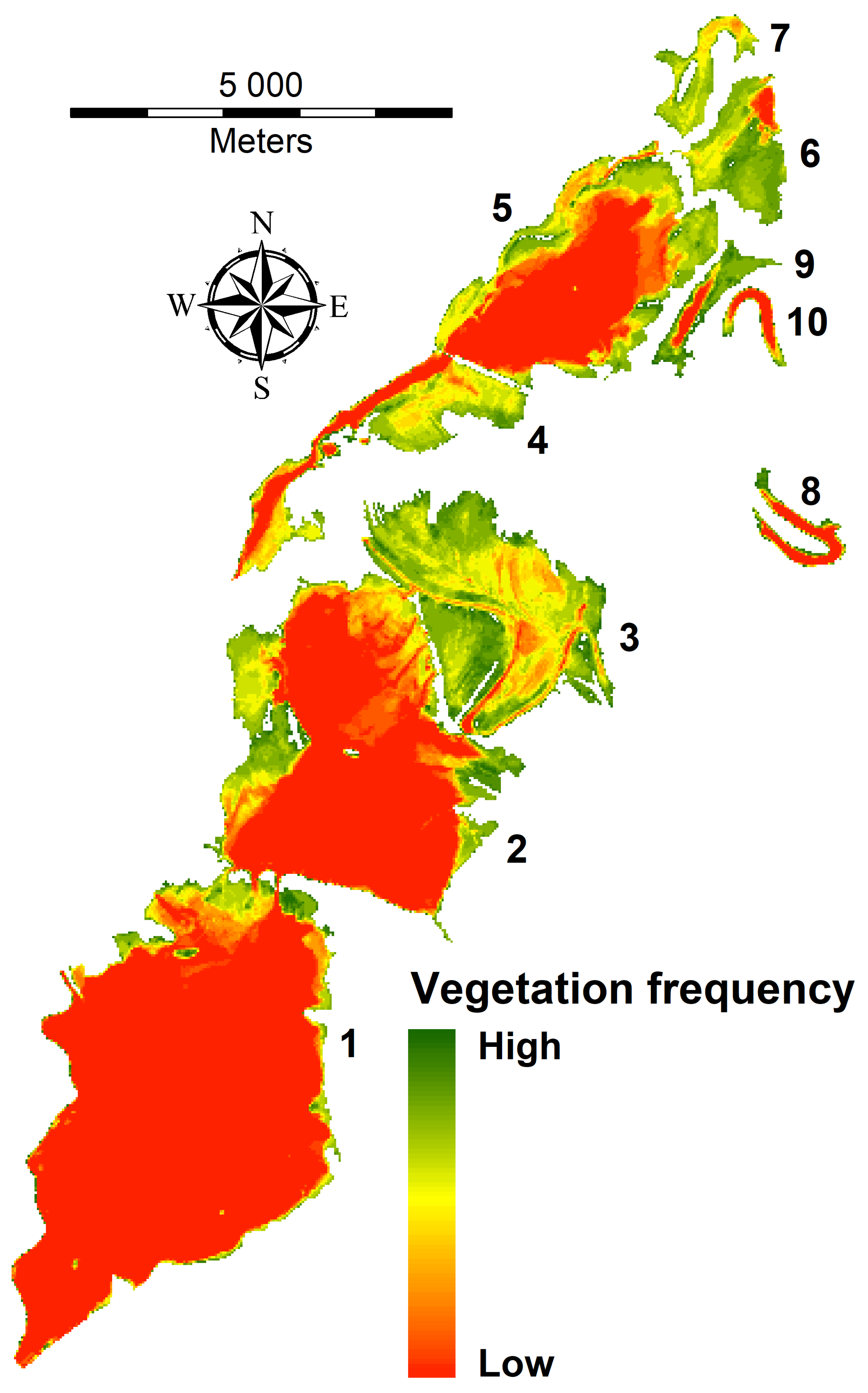
2.1. Study Area

The study area for this research was Lake Tisza, the second largest lake in Hungary (Figure 1). This lake is artificial, established in 1973 to facilitate flood control. There is a dam at Kisköre that is responsible for managing the water level. The area of the lake is 127 km2 and includes several islands (43 km2) that fragment the water surface into partly separated water sub-basins. The largest component of this lake consists of flooded former ploughed lands and orchards, and several flooded oxbow lakes and deeper depressions are also present, which means that average water depth is just 1.3 m; the deepest point of the lake is 17 m within a former oxbow. The water level is artificially regulated, depending partly on the discharge of the Tisza River (the lake is a buffer for floods, and thus can mitigate the water level in the lower river section), and partly on the demand for irrigation and nature conservation. Increasing the water operation level by 150 cm was planned in three stages (1973, 1980, and 1995), but the third stage was cancelled due to concerns about the stability of affected dykes and consideration of the additional disadvantages (e.g., raised groundwater and diminishing valuable habitats). The raising of the water level is undertaken gradually during each year. Generally, the water level is 2 m lower in the winter season (when gates are opened at the dam), and filling begins in February and ends at the middle of April. During this period, flood management results in the lake reaching its operation level and, thereafter, the water level is kept more or less stagnant (725 cm at Kisköre). According to operational requirements, the water level has been changed three times over the course of the period examined in this study: between 1984 and 1985 (675 cm; began in 1980 and ended in 1985); between 1986 and 2001 (727 cm); and between 2002 and 2017 (735 cm) (Figure 2). KÖTIVIZIG (Water Directorate of Central Tisza Region) provided the water level data used in this research. The zero points of the water level reported herein were collected at ‘Kisköre felső’ at 81.32 meters above sea level. This is the southernmost point of Lake Tisza at the Kisköre Dam; the data presented here can therefore describe water level conditions across the whole lake.
Floodplain forests, herbaceous and aquatic vegetation, and open waterbodies [49,50] are the most important land cover types of Lake Tisza. In spite of its artificial origin, Lake Tisza and surroundings comprises one of the most important wetlands in Hungary because it provides several semi-natural habitats for various species. This lake is a UNESCO World Heritage site as part of the Hortobágy National Park, a Ramsar Site, and part of the Natura 2000 Network (Tisza-tó Special Areas of Conservation). Long-duration floods leading to high water levels at the beginning of the vegetation period hinder the sprouting of plants; this is most obvious in the case of aquatic vegetation, but also affects other herbaceous plants and means that an open water surface will appear in commonly vegetated areas [51,52].
A number of factors endanger the persistence of Lake Tisza. The most significant issue is sedimentation, a consequence of high suspended sediment volumes. The presence of Kisköre dam means that suspended materials settle in the water basin and, thus, water depth decreases and provides more possibilities for the establishment of vegetation. Water caltrop (Trapa natans) is one of the dominant species in the lake; this plant floats on the water surface and has roots that extend deep under water. This plant is a protected and disappearing species across Europe [53] but in this lake it poses a threat to biodiversity and accelerates sedimentation. Water caltrop abundance also depends on water depth; when depth is greater than 2 m, plant density is suppressed but in shallow water this species covers large water surface areas. Macrophyte patchiness also affects hydraulics and, consequently, budgets of macroscale suspended particulate matter [54]. Thus, in shallow aquatic habitats where macrophytes can become established, changes in near-bed velocity will influence sediment transport and, as a result, lake bathymetry. These biogeomorphic feedback loops are important for macrophyte development [55].
Officially, the lake has 4 basins. In this study, one, Abádszalók basin, was completely omitted as it can be found in other paths of the Landsat imaging. However, as we intended to investigate local processes, we divided the remaining 3 basins into 10 units (ignoring the official nomenclature) based on physical properties rather than extent (i.e., larger flooded ploughlands—no. 1, 2, 5; or former oxbow lakes—no. 7, 8, 10). This approach ensured a more detailed spatial analysis, which had more relevance to the real circumstances as vegetation spread poses different risks in different basins (Figure 1; Table 1).

2.2. RS Images and Auxiliary Data

We used RS images from different Landsat sensors to observe land cover change across Lake Tisza, specifically Landsat 4, 5 Thematic Mapper (TM), Landsat 7 Enhanced Thematic Mapper Plus (ETM+), and Landsat 8 Operational Land Imager (OLI). All sensors have 30 m spatial resolution and similar spectral ranges, so we were able to compare images and results. We downloaded surface reflectance images (Level 2; L2) and NDVI composites (derived from L2 surface reflectance data) from the USGS ESPA ordering interface [56] and we calculated MNDWI composites from L2-level atmospherically corrected surface reflectance bands. KÖTIVIZIG (Water Directorate of Central Tisza Region) provided a digital bathymetry model which was used in the validation phase to confirm results. The model is a result of a 2-week field survey campaign in 2017, conducted with sonar devices mounted on boats, and discrete point measurements with Real-Time Kinematic Global Positioning System (RTK GPS). Then, the final model was generated with spatial interpolation of the data collected with the sonar devices and GPS (natural neighbor algorithm).

2.3. Data Pre-Processing

We initially determined the most appropriate period for time series analysis. This necessitated finding a year with the largest number of cloud-free images covering the vegetation period. We therefore chose 2015 for analysis as six images were available with the most favorable characteristics between May and September. We also sought the densest vegetation where the variance of NDVI values were smallest, i.e., the interquartile ranges of NDVI values showed the least variation, when restricted to the vegetated area using MNDWI <0 to exclude open water surfaces. Thus, we were able to focus on the vegetation density. On this basis, and taking into account revisiting times of Landsat satellites, we took into consideration all of the spatially and temporally available imagery. This resulted in 20 cloud-free images (based on visual selection and in case of Landsat 8 using the Cirrus band) captured between 1984 and 2017 that were used in this study (Figure 3, Table 2).

2.4. Data Processing

We restricted our analysis to the lake area regardless of aquatic vegetation cover, excluding terrestrial areas, and divided it into 10 water basins taking into account natural and artificial elements (Figure 1) using high resolution aerial images and topographic maps. The separation enabled us to reveal trends and the spatial distribution of changes in vegetation succession.
We utilized spectral indices to monitor aquatic vegetation spread over the open water surface and applied the previously downloaded NDVI (Equation (1), [57,58]) to quantify the greenness of pixels (i.e., green vegetation):
N D V I = N I R R E D N I R + R E D
In this expression, RED denotes the red band (i.e., band 3 for Landsat 4, 5, and 7 but band 4 for Landsat 8) while NIR denotes the infra-red band (i.e., band 4 for Landsat 4, 5 and 7 but band 5 for Landsat 8).
We calculated the MNDWI (Equation (2) [59]) to delineate open water surfaces, as follows:
M N D W I = S W I R G R E E N S W I R + G R E E N
In this expression, GREEN denotes the green band (i.e., band 2 for Landsat 4, 5 and 7 but band 3 for Landsat 8), while SWIR denotes the shortwave infra-red (i.e., band 5 for Landsat 4, 5, and 7 but band 6 for Landsat 8).
Although NDVI was used to identify aquatic vegetation, MNDWI provided a better index for determining open water surface [60,61]. Calculations were therefore performed in two steps. We initially calculated the mean, lower quartile (q1), median (q2), and upper quartile (q3) values for the NDVI in each year by water basin and then determined open water surfaces using MNDWI. We used a threshold value 0, according to Xu [59], to extract water features (where MNDWI values were greater than or equal to 0, negative values represented vegetated areas) and then repeated calculations of univariate statistics for these areas. For the methodological flowchart see Figure 3. We present our results as boxplot diagrams (Figure 4, Figure 5, Figure 6 and Figure 7) and evaluated them from three perspectives (Figure 3): we first determined NDVI by water basin as a whole and then divided the water basins into open water surfaces (i.e., MNDWI ≥ 0) and vegetated areas (i.e., MNDWI < 0). However, as available images were not equidistant, we did not apply formal time series analysis; graphical presentation nevertheless made it possible to draw conclusions regarding the changes in both vegetation and open water surfaces. We also derived a water depth model from these three perspectives (whole water basin, open water surface, and vegetated surface).
We determined vegetation frequency over the time series of this analysis by summarizing vegetated areas based on MNDWI indices (i.e., where MNDWI < 0), as each pixel that was not water was assessed as a vegetated area. Thus, using this frequency map we defined permanent open water surfaces (i.e., at least 18 times covered with water over the 20 investigated dates, 90%) and used vegetated areas as a counterpoint. We also determined the Percentage of Open Water (POW [%]; Equation (3)) as the ratio of open water and the whole area of a given water basin.
P O W   [ % ] = o p e n   w a t e r   a r e a   o f   a   b a s i n   [ m 2 ] w h o l e   a r e a   o f   a   b a s i n   [ m 2 ]
POW values were examined from the perspective of the relationship with the water level. Thus, July water levels (most of the satellite images were captured in this month) of each corresponding year were used in this analysis such that minimum (j_min), maximum (j_max), mean (j_mean), and standard deviation (j_sd) were calculated. Correlations were visualized using a correlation plot.
We utilized ENVI IDL 5.3 [62] and ArcGIS 10.4 [63] for image processing while the jmv package [64] of the software R 3.5.1 [65] was used for statistical analysis. Each index and result map derived from Landsat imagery has a 30 m Ground Sampling Distance (GSD).

2.5. Vegetation Spread Risk Mapping and the Level of Sedimentation Risk Index (LoSRI)

We calculated the risk of vegetation spread for each water basin as a measure of succession level and sedimentation. In other words, the higher the vegetation density, the higher the sedimentation, as deep water is not favorable for many plant species to occupy the open water surface (i.e., most plants, such as water caltrop and reeds, require shallow water). This means that the presence of aquatic plants indicates sedimentation and shallow water. Changes can be followed annually using a time series. We therefore specified threshold values for average NDVI (i.e., higher values indicate denser vegetation) and minimum POW (i.e., minimum POW appearance annually) to determine threat factors for water basins (Table 3). The two threat factors were assigned to each water basin; a summarized value specifies a level in each case based on the LoSRI (Equation (4)). These two factors can indicate very important components of lake sedimentation; the NDVI can measure vegetation density via the amount of biomass in a water basin (larger values indicate larger biomass), while the POW can show the ratio of unvegetated areas (the larger proportion of open water is more favorable).
Values for LoSRI were calculated as follows (Equation (4)):
L o S R I = V D F + O W F F
In this expression, LoSRI is the Level of Sedimentation Risk Index and VDF is the Vegetation Density Factor, i.e., the average NDVI of the observed years of a given water basin. Similarly, OWFF denotes the Open Water Fraction Factor, i.e., the proportion of water basin open water surface (Table 3). Values for this metric range between 2 and 12: thus, 2 indicates no risk and 12 indicates a very significant risk that this water body will disappear in the future.

2.6. Validation

In the frame of validation, we determined the Ratio Of the Vegetated areas and Water basins (ROVW). Vegetated water surface is the inverse of POW, and is determined as Equation (5):
R O V W   [ % ] = 100 P O W
ROVW, water depth and LoSRI values are depicted in the same figure with a double y-axis (see Section 3.6 below). The pattern of the values reflects the relationship. We also determined the correlation between LoSRI and water depth with Spearman’s rho, as LoSRI can be considered as an ordinal variable.

3. Results

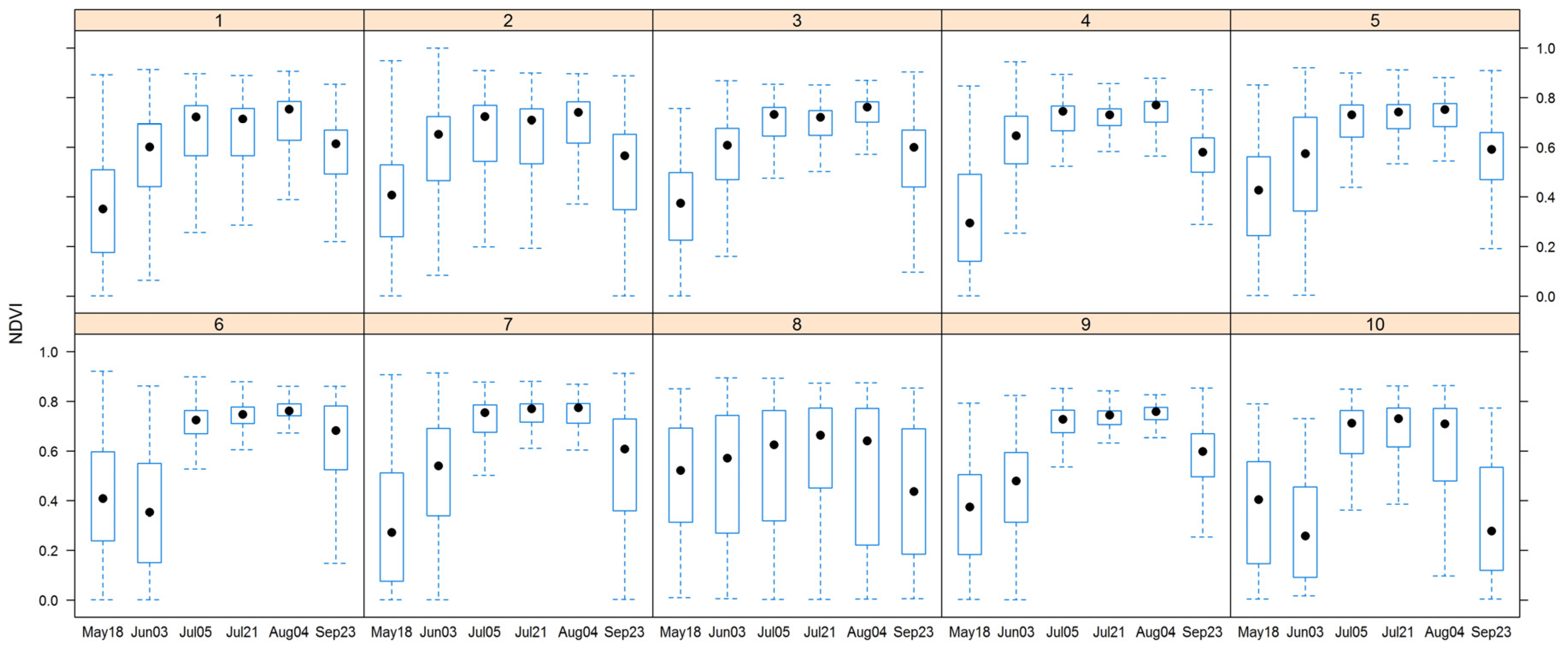
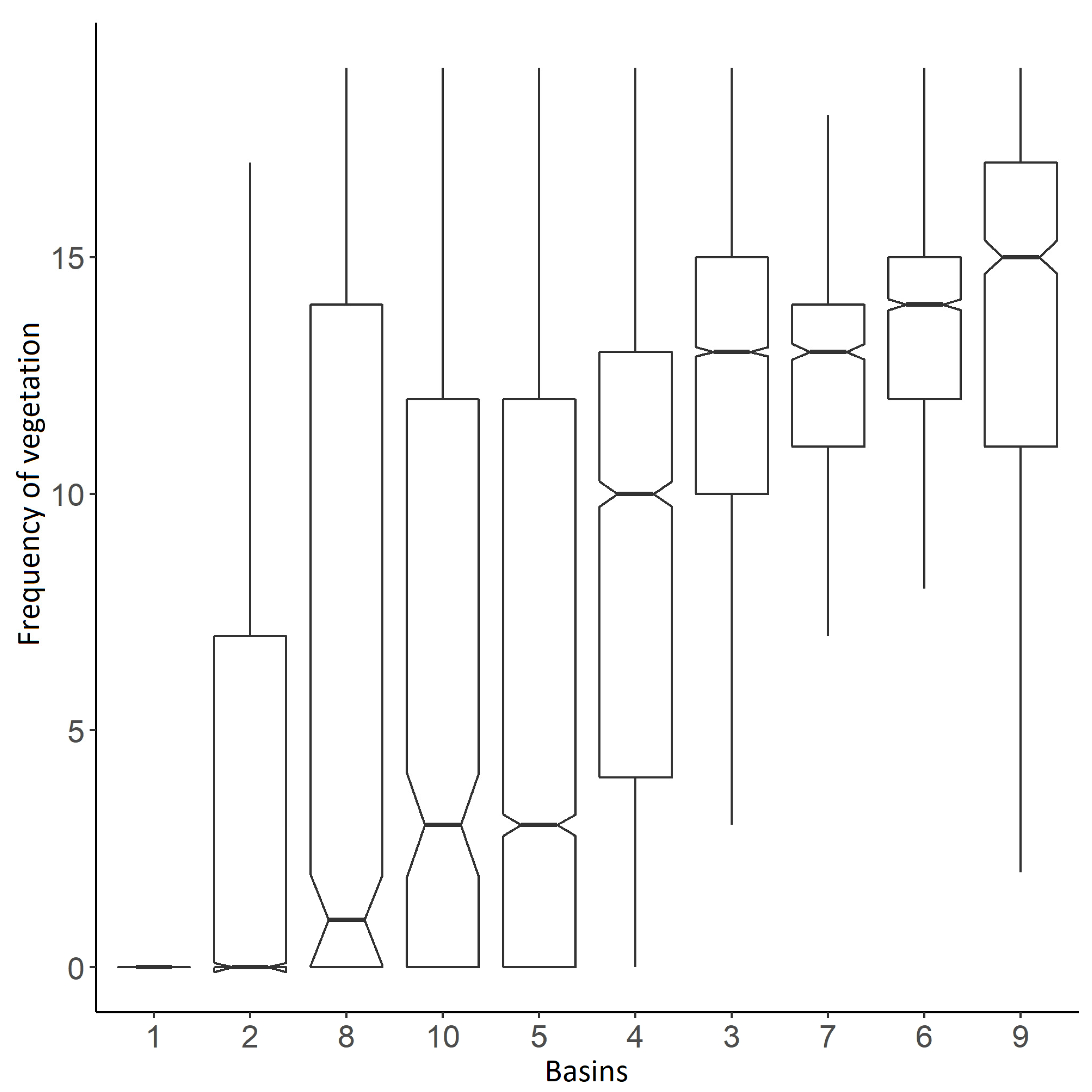
3.1. Aquatic Vegetation Annual Dynamics

The data presented here reveal an NDVI trend between May and September 2015, as we searched for vegetation maximum values that are highest and encompass the least variance. Data showed that each water basin within the sample area was characterized by similar succession dynamics; subsequent to 5 July, vegetation cover reached a maximum extent with high NDVI values, with the highest occurring on 4 August; the next image, on 23 September, shows that the vegetation started to collapse (Figure 4). Accordingly, the best period for sampling fell between 28 July and 11 August; we therefore focused on this period for further analyses.

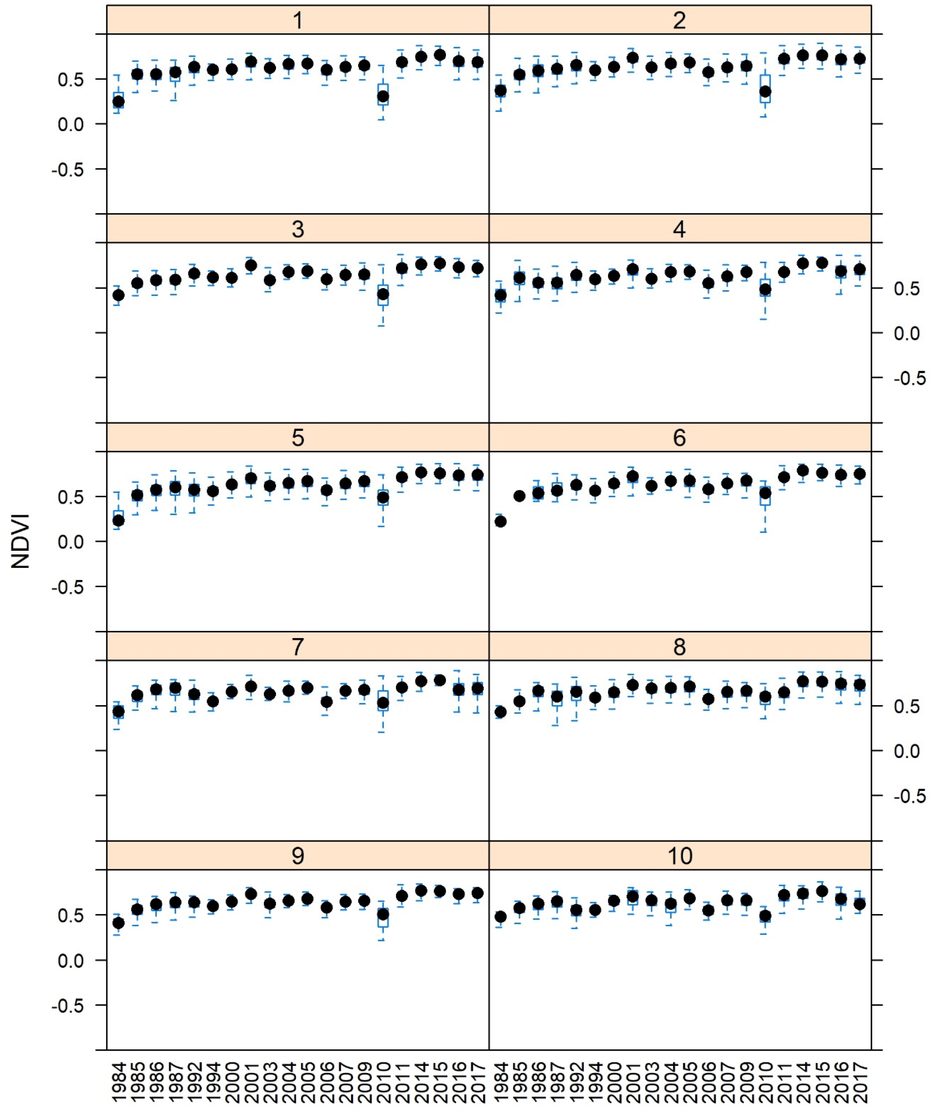
3.2. Aquatic Vegetation Dynamics Between 1984 and 2017

We distinguished three water basin trend types based on the variance (minimum, median, maximum) of NDVI values between 1984 and 2017 (Figure 5). The first of these comprised water basins 1, 2, and 5, as these exhibited decreasing trends in NDVI values between 1984 and 2015 before increasing again from 2015 onwards. Fluctuations were also seen over the study period, but this increase was significant in the case of water basin no. 5, for which the median NDVI rose above 0.5, suggesting extensive vegetation development. The second trend type we distinguished comprised water basins 3, 4, 6, 7, and 9; these water basins all generally exhibited increasing trends over the sampling period, taking the shape of saturation curves. Data showed that between 1984 and 1987, NDVI decreased, but began to increase between 1987 and 2000, following a steep curve, before values stagnated or showed a slight decrease. Water basins 8 and 10 represented the third type, where the NDVI values did not show a definite trend and medians fluctuated in a wide range, even in consecutive years. The year 2010, in particular, was outstanding in this sample, as NDVI values remained at their lowest compared to values in other years.
Next, we repeated our analyses for open water surfaces (MNDWI ≥ 0) as well as in areas of aquatic vegetation (MNDWI < 0). The results of this analysis enabled us to distinguish two trends in water surface NDVI values (Figure 6) with substantive differences between the two. The first type comprised water basins no. 1, 2, 4, and 5 and revealed a decreasing trend in NDVI values, as well as increasing values over the last three years between 2015 and 2017. In most years, however, NDVI values remained below zero and indicated open water. The second type (water basins no. 3, 6, 7, 8, 9, and 10) exhibited larger NDVI values and positive medians in most years. Water basins no. 3, 6, 7, and 8 all exhibited an increasing trend in the NDVI values between 1984 and 2000, while no. 9 and 10 were characterized by a stagnant but fluctuating trend.
Analysis showed that vegetated areas exhibited very similar trends among the different water basins based on statistical analyses of NDVI values (Figure 7); we were therefore unable to separate different trend types. There was an increasing trend in the NDVI values with two minimum points at 1984 and 2010. Subsequent to 2014 there was a very slight decreasing trend in NDVI values.

3.3. Changes in Open Waterbody Ratios

The water basins analyzed here comprised five different types based on open waterbody percentages (Figure 8). The first type (#1) is seen in water basin no. 1 where there was a slight decrease overall, reaching a maximum value in 2010. This conspicuous year was observable in each water basin, while the second type (#2) was comprised of water basins 2 and 5. A decreasing trend was evident between 1984 and 2005, the ratio then increased up to 2010, before a reductive process began. The ratios in each case also remained higher than 50%, while the third type (#3) was comprised of water basins no. 3, 6, and 7. Trends in this case were similar to those seen in type #2, although minimum percentage values approached zero between 2000 and 2005. In the fourth type (#4) were water basins no. 4 and 9, while the fifth type (#5) comprised no. 8 and 10, where trends were similar to those seen in type #3 in which ratios encompassed a larger variance. Minimum values in this case did not approach zero.
We then summed the vegetated areas over the course of this survey (Figure 9). Considering median vegetation frequencies, two clusters were recovered, namely, medians below 3, in the case of water basins no. 1, 2, 5, 8, and 10, with lesser risk of complete occupation by aquatic plants; and medians above 10, in water basins no. 3, 4, 6, 7, and 9. This latter group was at considerable risk (Figure 10).

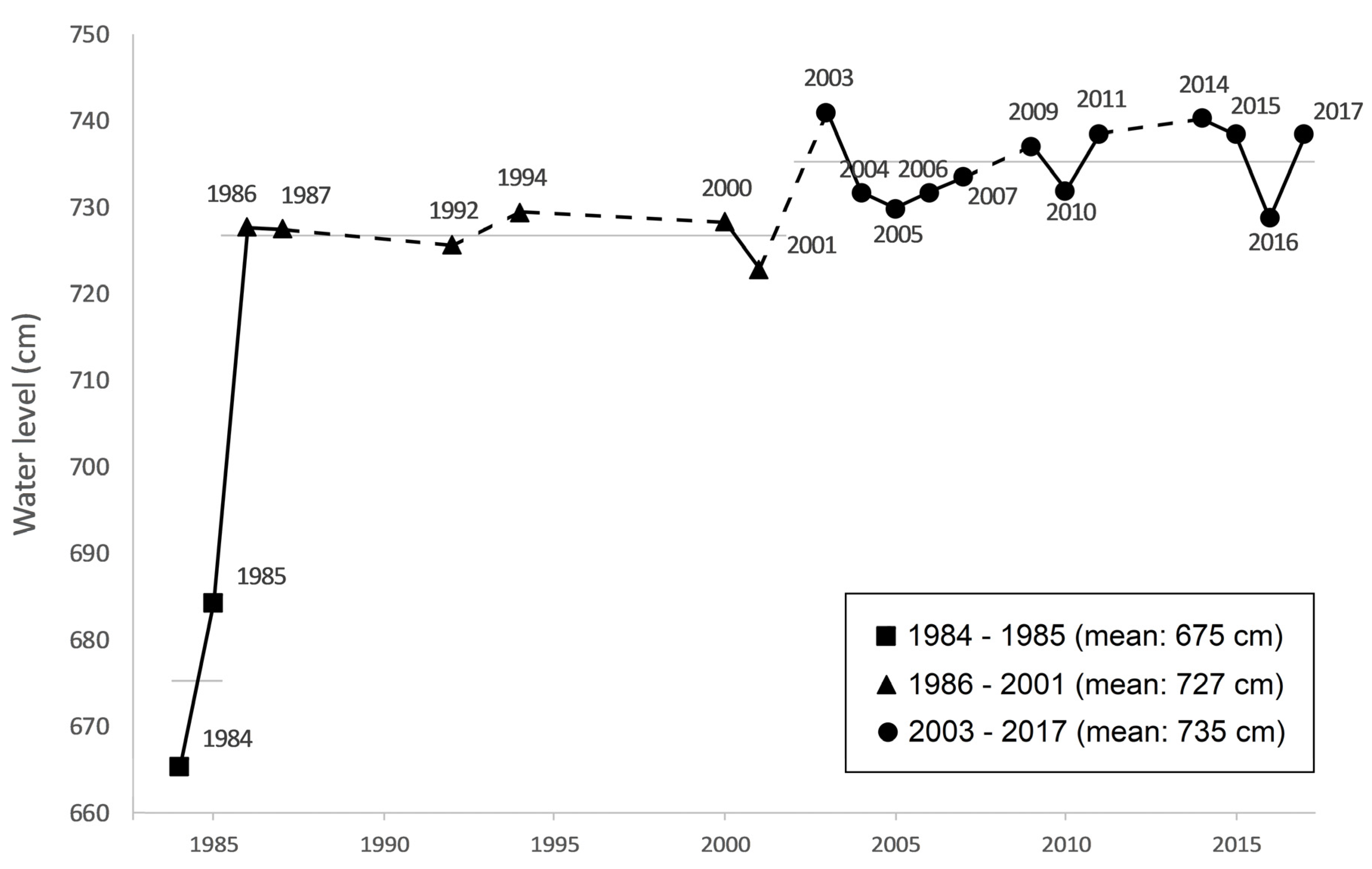
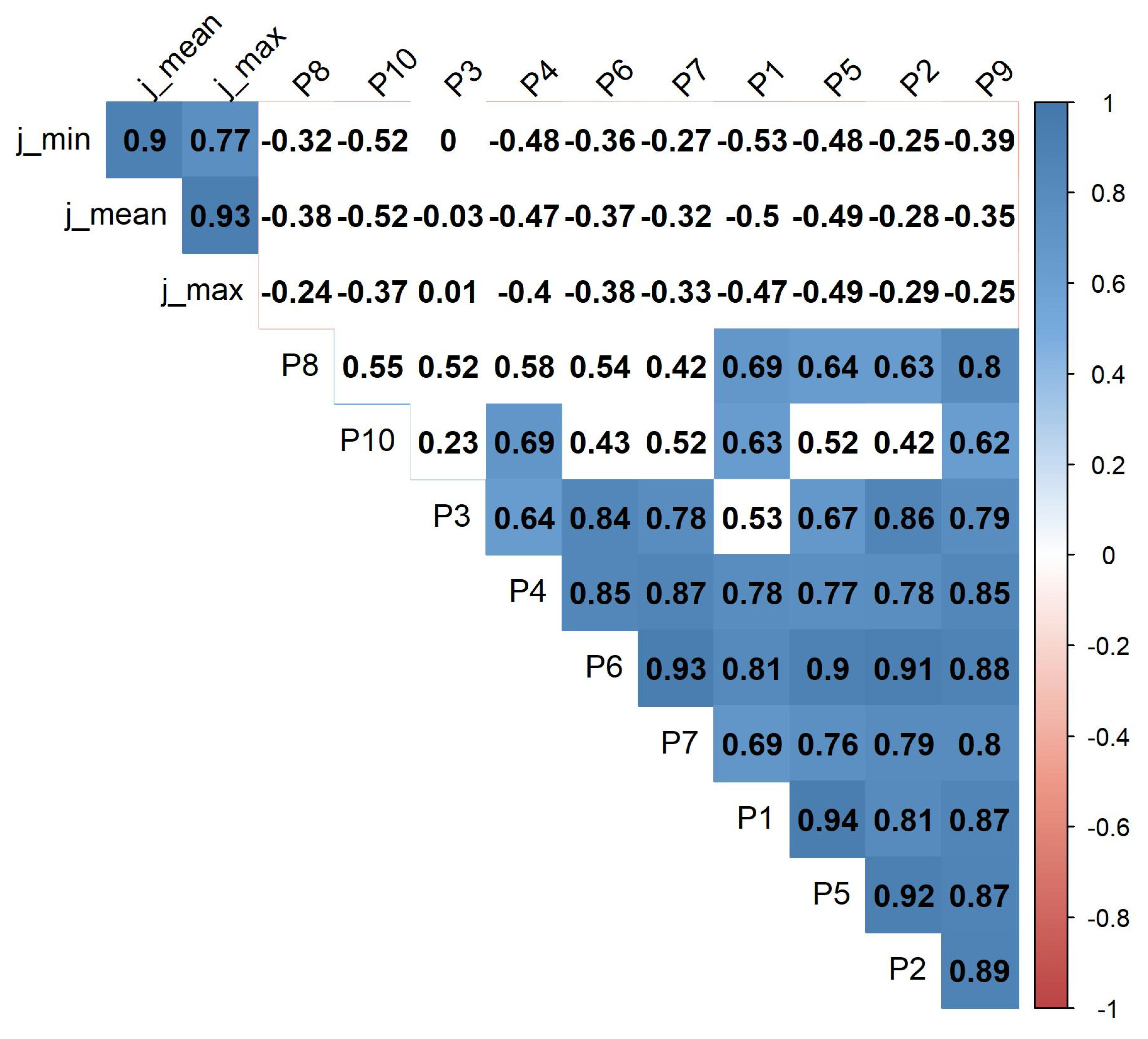
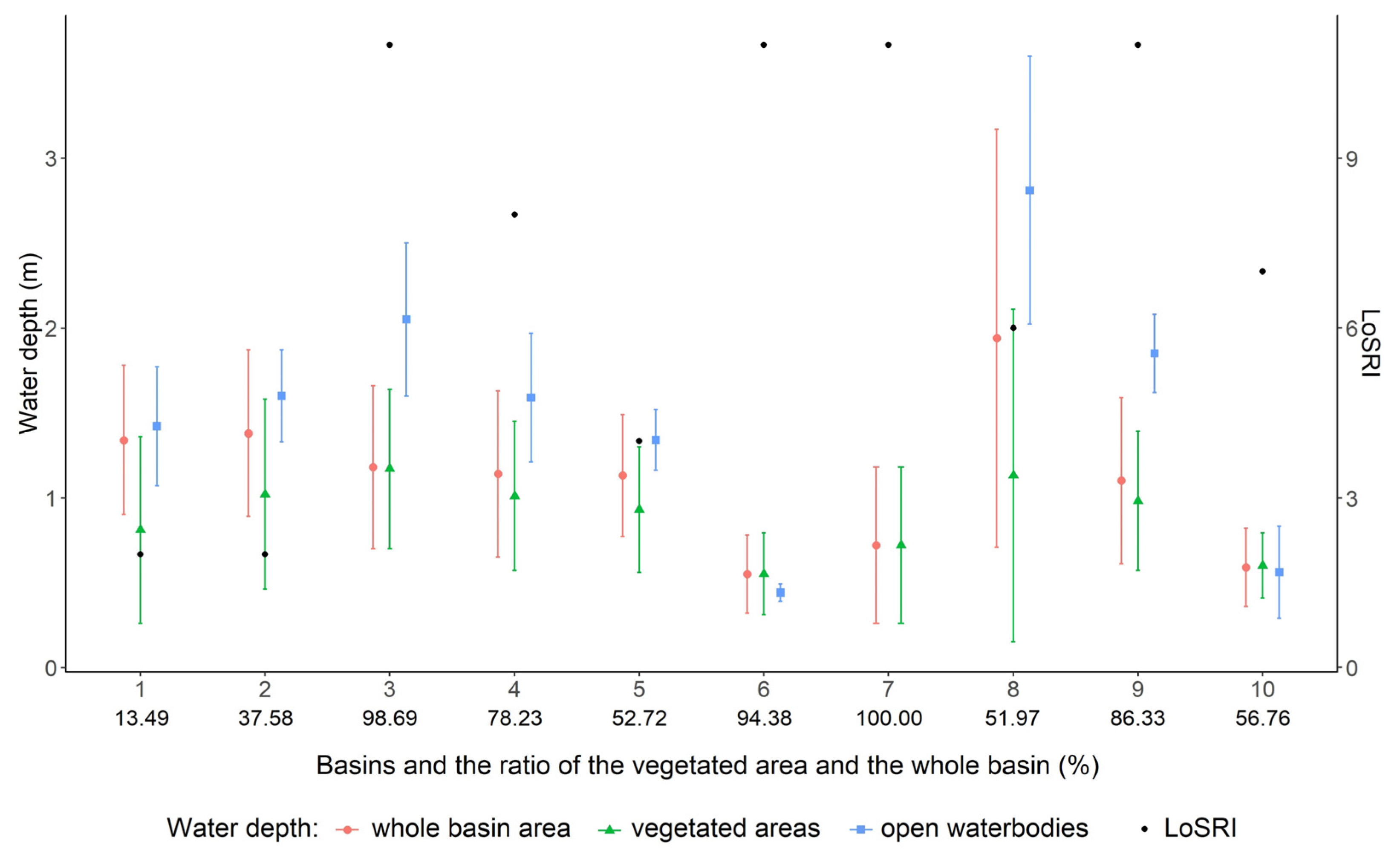
3.4. The Relationship Between POW and Water Level

Water levels were 665 cm, and 685 cm in 1984 and 1985, respectively, while in consecutive years the level was operationally increased to around 725 cm. We therefore excluded 1984 and 1985 from the analysis in order to avoid generating false conclusions. Correlations between water level and POW fell between 0.00 and −0.53 even though these relationships were not significant (Figure 11) because of low sample size. We cannot consider these results to be representative of accurate outcomes: the low variance related to POW water level remains insignificant, while the relatively large correlations (between ca. 0.50 and 0.94) between water level values of studied water basins indicate that water level is very similar across the whole area within the reservoir. The only exceptions were water basins no. 8 and 10, both oxbow lakes, which are rather isolated in their situation and whose water budgets are independent of the regulated water table.

3.5. Sedimentation Risk Mapping

We separated water basins that are differently threatened in this analysis using the LoSRI index (Table 4). Our results show that, first, the less-threatened water basins are no. 1, 2, and 5, which are large and deep enough to hinder the establishment of aquatic vegetation, including water caltrop. These water basins had low average NDVI values (less than 0.15) and, no. 1 and 2, in particular, had high open-water ratios (greater than 65%). We also show that water basins no. 4, 8, and 10 had medium average NDVI values (0.3–0.4), while water basins no. 8 and 10 had POW values above 35%. These water basins were not greatly influenced by succession. The most threatened water basins within our sample were no. 3, 6, and 7. These water basins had extremely high NDVI values (all greater than 0.45) and reached almost zero open water percentage values in some years during the 2000s. These water basins were most affected by succession. Water basin no. 9 also had a high average NDVI value (0.51) during the studied years. This water basin was formerly a river meander, as was also the case with water basins no. 8 and 10; these were therefore deeper and, as a result, aquatic vegetation could not spread efficiently. However, in the latter years of this study, the open water percentage of water basin no. 9 decreased from an average of 20% to 13%. It is therefore worth considering that this water basin is threatened.

3.6. Validation

The LoSRI was developed in order to predict future changes including the spread of aquatic vegetation. The Spearman correlation was 0.60 (p < 0.05) between the LoSRI and average water depth taking into account all samples. Average water depth in the largest water basins (no. 1 and 2) was less than 1.4 m while open waterbodies were 1.42 m and 1.60 m in depth (Figure 12). These water basins also had small (13.49% and 37.58%) ROVWs and the smallest LoSRI values (i.e., equal to 2). Former river meanders (no. 3, 8, and 9) had the highest average water depths of open waterbodies (>1.85 m) and, because of their small POW and high ROVW values (greater than 51.97%), these are threatened by succession, particularly water basins no. 3 and 9 (ROVW values greater than 86.33%). The LoSRI values in this case were also high (i.e., equal to 11); water basins no. 6, 7, and 10 had shallow average water depths between 0.55 and 0.72 m, while water basins no. 6 and 7 had ROVW values above 94%. These water basins also had very high LoSRI values (i.e., equal to 11); water basin no. 7 was completely covered by vegetation while no. 6 had a minimal permanent open water surface area and a low (0.44 m) water depth. Although water basin no. 10 was a former meander, its average depth was only 0.59 m. This water basin also had a 56.76% ROVW value and a LoSRI equal to just 7.

4. Discussion

Indicating water depth is a challenging topic, but as depth is an important driver of vegetation spread and shallow water is favorable for several plant species, depth can be indicated by aquatic vegetation. Moreover, NDVI can be an effective tool, as a proxy, to monitor vegetation spread and sedimentation. The Tisza River transports large volumes of suspended sediments [66], which are then deposited within the water basins of Lake Tisza due to changing flow conditions. Due to the effect of the Kisköre dam, the water flow in the basins is minimal; thus, the lake faces sedimentation, favorable for the establishment and spread of aquatic vegetation (mostly water caltrop and duckweed), as well as species typical in shallow water (e.g., reed mace). Accordingly, the lake is losing open water areas [49,67]. From the present study, trends did not indicate severe risk, however, although aquatic vegetation and shoreline herbaceous plants surface processes did not show evidence of intensive spreading, it was found that POW values can fluctuate by more than 50% due to flooding (Figure 8). Management by cutting machines and large floods (for example in 2010) at the beginning of the vegetation period when the water table was higher hindered the spread of aquatic vegetation. Plants were not able to sprout and this caused a negative anomaly in the NDVI values (Figure 5 and Figure 6). Sedimentation remains a problem endangering the existence of the lake in the long run, and the oxbows are also endangered [68].
We discriminated three types of water basins within our study area on the basis of the observed NDVI dynamics, in high accordance with extent and depth. Large basins were characterized by open water surfaces, deep water, and minimal vegetation coverage. The smaller water basins comprised oxbows and paleo-channels with the deepest water. These smaller basins varied in indices and mostly had positive NDVI values with larger variance. Water caltrop requires a water level less than 2 m in depth, although other aquatic species such as duckweed were dominant in some years. In cases where water basins contained shallow water (less than 1.3 m), water caltrop occupied large areas. Excluding vegetated areas from NDVI statistics, we were able to delineate two water basin types based on quantitative differences. Water basins no. 1, 2, 4, and 5 mostly had NDVI values below zero, which means that they had more open water surface than the other basins (no. 3, 6–10). Observations of NDVI for the vegetated areas (Figure 7) resulted in just one class, which indicates that vegetated areas are homogenous.
The five separated types of POW values resulted in more variation in the water basins within our sampling area in terms of NDVI. We were also able to show that MNDWI values provide an effective tool to determine POW and, with NDVI, enable us to provide information on qualitative conditions of the vegetated areas within water basins. The levels of vegetation cover in water basins over the years studied here refer to trends in succession.
No previous study has been devoted to Lake Tisza succession and just a handful have so far focused on average sedimentation rates in other parts of the river and floodplain. According to 137Cs (radioactive isotope of cesium) measurements, researchers have used experimental nuclear tests based on the marker layer laid down by the Chernobyl accident in 1986. The sedimentation rate in oxbow lakes is between 1 and 2 cm/year but, with large floods, can exceed 5 cm/year [33,69]. Oxbows act like sediment traps related to other parts of the floodplain because of hydrodynamic forces. Sedimentation speed is also a function of distance from the river; over shorter distances, this rate is between 1 and 2 cm/year, while above 200 m it decreases to 0.4 cm/year [70]. It is also noteworthy that there are a number of discrepancies with the observations presented here; for example, because Lake Tisza comprises a set of water basins connected with canals, the coarse fraction of suspended sediment will be deposited immediately when the speed of the flow decreases. This also refers to the largest sedimentation volumes; contrary to oxbows situated on floodplains, those in Lake Tisza might not be the most intensive parts to sedimentation.
Although previous studies have noted a correspondence between NDVI and water level (e.g., Omute et al. [44]), we were unable to confirm this relationship in this analysis. We do know if the operational water level changes according to actual management aims; this level rose 60 cm between 1984 and 1986. A correlation analysis performed on our dataset including 1984 and 1985 showed a significant negative relationship, with r values were between −0.7 and −0.9. This indicates that higher water levels had a good relationship with smaller POW values. The explanation for this is complex for two reasons: first, at the beginning of reservoir operation, the presence of aquatic vegetation was not typical; and second, higher water levels have impeded the spread of water caltrop (Trapa natans), which poses the largest threat regarding vegetation spread in the lake. POW values should be higher with higher water levels when all other circumstances remain constant. Correlations between POW and the water level excluding 1984 and 1985 remained significant with r > 0.5; this is one consequence of the small variance in water level values (standard deviation: 5.4 cm). One breakpoint was observed in 2002 when the water level rose an additional 10 cm.
Previous studies have shown that water caltrop is the most abundant plant in water depths of 2 m [53]. Future work should also take herbaceous and aquatic plants into account, but our results showed that mean water depth in vegetated areas was 0.88 ± 0.47 m. This means that vegetation can spread easily in these parts of the water basins. Mean water depth in open waterbodies remained within 1.52 ± 0.33 m. The presence of aquatic vegetation, in this case dominated by water caltrop, depends on water depth, which is affected by two key parameters: the regulated water level and sedimentation. We have therefore been able to show that aquatic vegetation is an effective indicator of water depth.
The correlation between LoSRI and mean water depth within the water basins studied here was 0.6 (p < 0.01). This result means that LoSRI can provide indirect information about water depth based on only satellite imagery because NDVI evaluates the state of water basins based on the open water surface quantity (POW) and biomass amount. These factors are the consequences of water depth. Thus, shallower water basins usually have higher LoSRI values while deeper water basins have smaller values. It is also necessary to consider ROVW values because a water basin with shallow water can also contain a large open waterbody due to management, the presence of a former meander, or the topography of a particular water basin. In conjunction, LoSRI and ROVW can predict the state of water basin sedimentation. It should be noted that the correlation between LoSRI and water depth (r = 0.6) was moderate. This moderate level of correlation might be due to the fact that water depth reflected only the current status (a single survey in 2017) of the lake-bed, while the LoSRI was calculated with 20 satellite images of a time series covering 33 years. In addition, the lake is under continuous water level regulation, and some areas receive plant-cutting treatment using aquatic plant harvester machines.
LoSRI can be an efficient indicator for most lake basins. However, for oxbows and paleo-river meanders, where the basin area is smaller and the water depth can be significantly higher, LoSRI overpredicts risk, as deeper inner parts are not threatened, only coastal regions. This may be the case with water basins no. 8, 9, and 10, in which the water depth is the greatest and only the littoral zone can be vegetated as water deepens within a short distance; i.e., the succession process is relatively long. In addition to the LoSRI index, a vegetation frequency map should therefore also be used in these cases. This approach helps to identify permanent open waterbodies that are not currently threatened by succession and also only requires satellite images from an area with no additional data input. This workflow is therefore efficient and can be quickly applied to a specific area where succession is suspected.
Kiage and Douglas [60] also applied MNDWI and NDVI, and found that MNDWI provides more reliable results compared to NDVI; in our methodology, we used MNDWI to identify water surfaces and NDVI was used to calculate biomass. However, further comparison with the similarities or differences of other authors’ findings is difficult, as studies dealing with lakes and wetlands are usually performed at the catchment level, or larger areas, and aim to reveal change in land cover categories and its consequences [71,72,73].
Sedimentation exerts a considerable effect on lake succession through sediment deposition and providing habitats for aquatic plants, which themselves accelerate sedimentation. It is therefore crucial to collect enough information about water depth. In most cases, authorities and lake managers simply do not have enough detailed information about the nature of the bottom of lakes and basins, and this remains difficult to determine, even with sonar devices, as depth changes due to sedimentation. Satellites can provide information on vegetation spread and integrate image interpretations with field vegetation surveys, thus making all of the collected information available for risk mapping. Our approach can work for shallow lakes, and requires knowledge of plant species and long-term satellite imagery. These requirements, as well as our new approach, means that the locations of shallow water bodies and sedimentation rates can be estimated using only satellite images. Although the study’s validation resulted in only moderate correlations, better results could be achieved in water bodies where the water level is natural, and vegetation is not treated. In our case, it was important to find the hot spots of vegetation spread. Stationary open water surfaces and changes in vegetation cover are good indicators of risk. This result suggests a possible approach for water directorates to focus on endangered areas.

5. Conclusions

We performed a long term (1984–2017) vegetation change monitoring study based on Landsat image spectral indices for the Lake Tisza area, Hungary, with the aim of revealing if a trend exists in vegetation spread at the sub-basin level (in 10 water basins), and to develop a methodology to identify the sub-basins where the sedimentation-related vegetation spread poses a risk. We determined NDVI values in the 10 water basins and separated the open waterbodies and vegetated areas by water basins based on the MNDWI index. Our results enabled us to specify six threat level factors for NDVI and POW values that were assigned to each water basin. LoSRI index values were then summarized from these data. Water level and water depth values were consistent with our results. Less-threatened water basins were the larger basins with low NDVI and high POW values, while the most threatened were smaller or more vegetated areas with high NDVI and low POW values. These water basins will require special management. Validation showed that there are limitations of the general usage of the LoSRI, but the moderate relationship indicated that with careful interpretation, the risk of sedimentation can be estimated. Plotting the summarized binary layers of the 20 satellite images of vegetation frequency based on MNDWI < 0 provided the possibility of spatial evaluation. As Lake Tisza is subject to regular human intervention (excavating sediment, harvesting plants, and artificial regulation of the water level), the trends of the water basins were not obvious. This method can be applied to large lakes to help identify sedimentation, but is limited to shallow lakes in which vegetation that favors shallow water is present. If these circumstances exist, sedimentation risk can be revealed.

Author Contributions

Conceptualization, L.S. and S.S.; methodology, L.S., S.S. and G.J.D.; software, L.S., T.B. and S.S.; validation, B.D. and T.B.; formal analysis, L.S. and G.J.D.; investigation, L.S., S.S., B.D., T.B. and G.J.D.; resources, S.S. and B.D.; data curation, L.S., S.S. and T.B.; writing—original draft preparation, L.S., S.S., B.D., T.B. and G.J.D.; visualization, L.S., B.D. and S.S.; supervision, S.S. and G.J.D. All authors have read and agreed to the published version of the manuscript.

Funding

The research was financed by the Higher Education Institutional Excellence Programme (NKFIH-1150-6/2019) of the Ministry of Innovation and Technology in Hungary, within the framework of the 4th thematic programme of the University of Debrecen. B.D. was supported by the NKFI KH 130338 and the NKFI FK 124404 projects. The project was supported by the Bolyai János Research Scholarship of the Hungarian Academy of Sciences (B.D.).

Acknowledgments

We would also like to show our gratitude to László Kummer, Head of Geoinformatics Division, KÖTIVIZIG Water Directorate for the supplemental data during the course of this research.

Conflicts of Interest

The authors declare no conflict of interest.

References

  1. Gulácsi, A.; Kovács, F. Drought Monitoring of Forest Vegetation using MODIS-Based Normalized Difference Drought Index in Hungary. Hung. Geogr. Bull. 2018, 67, 29–42. [Google Scholar] [CrossRef] [Green Version]
  2. Mas, J. Monitoring Land-Cover Changes: A Comparison of Change Detection Techniques. Int. J. Remote Sens. 1999, 20, 139–152. [Google Scholar] [CrossRef]
  3. Meyer, W.B.; Turner, B.L. Human Population Growth and Global Land-use/cover Change. Annu. Rev. Ecol. Syst. 1992, 23, 39–61. [Google Scholar] [CrossRef]
  4. Regmi, P.; Grosse, G.; Jones, M.C.; Jones, B.M.; Anthony, K.W. Characterizing Post-Drainage Succession in Thermokarst Lake Basins on the Seward Peninsula, Alaska with TerraSAR-X Backscatter and Landsat-Based NDVI Data. Remote Sens. 2012, 4, 3741–3765. [Google Scholar] [CrossRef] [Green Version]
  5. Sterling, S.M.; Ducharne, A.; Polcher, J. The Impact of Global Land-Cover Change on the Terrestrial Water Cycle. Nat. Clim. Chang. 2013, 3, 385–390. [Google Scholar] [CrossRef]
  6. Galat, D.L.; Verdin, J.P.; Sims, L.L. Large-Scale Patterns of Nodularia Spumigena Blooms in Pyramid Lake, Nevada, Determined from Landsat Imagery: 1972–1986. Hydrobiologia 1990, 197, 147–164. [Google Scholar] [CrossRef]
  7. Han, X.; Chen, X.; Feng, L. Four Decades of Winter Wetland Changes in Poyang Lake Based on Landsat Observations between 1973 and 2013. Remote Sens. Environ. 2015, 156, 426–437. [Google Scholar] [CrossRef]
  8. Yuan, F.; Sawaya, K.E.; Loeffelholz, B.C.; Bauer, M.E. Land Cover Classification and Change Analysis of the Twin Cities (Minnesota) Metropolitan Area by Multitemporal Landsat Remote Sensing. Remote Sens. Environ. 2005, 98, 317–328. [Google Scholar] [CrossRef]
  9. Claverie, M.; Ju, J.; Masek, J.G.; Dungan, J.L.; Vermote, E.F.; Roger, J.; Skakun, S.V.; Justice, C. The Harmonized Landsat and Sentinel-2 Surface Reflectance Data Set. Remote Sens. Environ. 2018, 219, 145–161. [Google Scholar] [CrossRef]
  10. Pahlevan, N.; Chittimalli, S.K.; Balasubramanian, S.V.; Vellucci, V. Sentinel-2/Landsat-8 Product Consistency and Implications for Monitoring Aquatic Systems. Remote Sens. Environ. 2019, 220, 19–29. [Google Scholar] [CrossRef]
  11. Foster, C.; Hallam, H.; Mason, J. Orbit Determination and Differential-Drag Control of Planet Labs Cubesat Constellations. arXiv preprint arXiv:1509.03270 2015. Available online: https://arxiv.org/pdf/1509.03270.pdf (accessed on 31 January 2020).
  12. Thenkabail, P.S. Remotely Sensed Data Characterization, Classification, and Accuracies; CRC Press, Taylor & Francis Group: Boca Raton, FL, USA, 2015. [Google Scholar]
  13. Zhao, B.; Yan, Y.; Guo, H.; He, M.; Gu, Y.; Li, B. Monitoring Rapid Vegetation Succession in Estuarine Wetland using Time Series MODIS-Based Indicators: An Application in the Yangtze River Delta Area. Ecol. Ind. 2009, 9, 346–356. [Google Scholar] [CrossRef]
  14. Lambin, E.F.; Turner, B.L.; Geist, H.J.; Agbola, S.B.; Angelsen, A.; Bruce, J.W.; Coomes, O.T.; Dirzo, R.; Fischer, G.; Folke, C. The Causes of Land-use and Land-Cover Change: Moving Beyond the Myths. Glob. Environ. Chang. 2001, 11, 261–269. [Google Scholar] [CrossRef]
  15. Turner, B.; Meyer, W.B.; Skole, D.L. Global Land-use/land-Cover Change: Towards an Integrated Study. Ambio.Stockholm 1994, 23, 91–95. [Google Scholar]
  16. Deák, B.; Valkó, O.; Török, P.; Kelemen, A.; Tóth, K.; Miglécz, T.; Tóthmérész, B. Reed Cut, Habitat Diversity and Productivity in Wetlands. Ecol. Complex. 2015, 22, 121–125. [Google Scholar] [CrossRef]
  17. Russell, M.; Fulford, R.; Murphy, K.; Lane, C.; Harvey, J.; Dantin, D.; Alvarez, F.; Nestlerode, J.; Teague, A.; Harwell, M. Relative Importance of Landscape Versus Local Wetland Characteristics for Estimating Wetland Denitrification Potential. Wetlands 2019, 39, 127–137. [Google Scholar] [CrossRef]
  18. Weller, M.W. Wetland Birds: Habitat Resources and Conservation Implications; Cambridge University Press: Cambridge, UK, 1999. [Google Scholar]
  19. Matthews, J.W.; Endress, A.G. Rate of Succession in Restored Wetlands and the Role of Site Context. Appl. Veg. Sci. 2010, 13, 346–355. [Google Scholar] [CrossRef]
  20. Östlund, C.; Flink, P.; Strömbeck, N.; Pierson, D.; Lindell, T. Mapping of the Water Quality of Lake Erken, Sweden, from Imaging Spectrometry and Landsat Thematic Mapper. Sci. Total Environ. 2001, 268, 139–154. [Google Scholar] [CrossRef]
  21. Rembold, F.; Carnicelli, S.; Nori, M.; Ferrari, G.A. Use of Aerial Photographs, Landsat TM Imagery and Multidisciplinary Field Survey for Land-Cover Change Analysis in the Lakes Region (Ethiopia). Int. J. Appl. Earth OBS 2000, 2, 181–189. [Google Scholar] [CrossRef]
  22. Scheffer, M.; van Nes, E.H. Shallow lakes theory revisited: Various alternative regimes driven by climate, nutrients, depth and lake size. In Shallow Lakes in a Changing World; Springer: Dordrecht, The Netherlands, 2007; pp. 455–466. [Google Scholar]
  23. Tanos, P.; Kovács, J.; Kovács, S.; Anda, A.; Hatvani, I.G. Optimization of the Monitoring Network on the River Tisza (Central Europe, Hungary) using Combined Cluster and Discriminant Analysis, Taking Seasonality into Account. Environ. Monit. Assess. 2015, 187, 575. [Google Scholar] [CrossRef]
  24. Csáki, P.; Szinetár, M.M.; Herceg, A.; Kalicz, P.; Gribovszki, Z. Climate Change Impacts on the Water Balance-Case Studies in Hungarian Watersheds. Időjárás Q. J. Hung. Meteorol. Serv. 2018, 122, 81–99. [Google Scholar] [CrossRef] [Green Version]
  25. Farkas, J.Z.; Hoyk, E.; Rakonczai, J. Geographical Analysis of Climate Vulnerability at a Regional Scale: The Case of the Southern Great Plain in Hungary. Hung. Geogr. Bull. 2017, 66, 129–147. [Google Scholar] [CrossRef] [Green Version]
  26. Babka, B.; Futó, I.; Szabó, S. Seasonal Evaporation Cycle in Oxbow Lakes Formed Along the Tisza River in Hungary for Flood Control. Hydrol. Process. 2018, 32, 2009–2019. [Google Scholar] [CrossRef] [Green Version]
  27. Csete, M.; Pálvölgyi, T.; Szendrő, G. Assessment of Climate Change Vulnerability of Tourism in Hungary. Reg. Environ. Chang. 2013, 13, 1043–1057. [Google Scholar] [CrossRef]
  28. Rátz, T.; Vizi, I. The Impacts of Global Climate Change on Water Resources and Tourism: The Responses of Lake Balaton and Lake Tisza. Adv. Tour. Climatol. 2004, 82–89. [Google Scholar]
  29. Zlinszky, A.; Mücke, W.; Lehner, H.; Briese, C.; Pfeifer, N. Categorizing Wetland Vegetation by Airborne Laser Scanning on Lake Balaton and Kis-Balaton, Hungary. Remote Sens. 2012, 4, 1617–1650. [Google Scholar] [CrossRef] [Green Version]
  30. Sándor, A.; Kiss, T. Floodplain Aggradation Caused by the High Magnitude Flood of 2006 in the Lower Tisza Region, Hungary. J. Environ. Geogr. 2008, 1, 31–39. [Google Scholar]
  31. Grygar, T.M.; Elznicová, J.; Kiss, T.; Smith, H. Using Sedimentary Archives to Reconstruct Pollution History and Sediment Provenance: The Ohře River, Czech Republic. Catena 2016, 144, 109–129. [Google Scholar] [CrossRef]
  32. Latuso, K.D.; Keim, R.F.; King, S.L.; Weindorf, D.C.; DeLaune, R.D. Sediment Deposition and Sources into a Mississippi River Floodplain Lake; Catahoula Lake, Louisiana. Catena 2017, 156, 290–297. [Google Scholar] [CrossRef]
  33. Nguyen, H.; Braun, M.; Szaloki, I.; Baeyens, W.; Van Grieken, R.; Leermakers, M. Tracing the Metal Pollution History of the Tisza River through the Analysis of a Sediment Depth Profile. Water Air Soil Pollut. 2009, 200, 119–132. [Google Scholar] [CrossRef]
  34. Hubay, K.; Molnár, M.; Orbán, I.; Braun, M.; Bíró, T.; Magyari, E. Age–depth Relationship and Accumulation Rates in Four Sediment Sequences from the Retezat Mts, South Carpathians (Romania). Quat. Int. 2018, 477, 7–18. [Google Scholar] [CrossRef]
  35. Babcsányi, I.; Tamás, M.; Szatmári, J.; Hambek-Oláh, B.; Farsang, A. Assessing the Impacts of the Main River and Anthropogenic use on the Degree of Metal Contamination of Oxbow Lake Sediments (Tisza River Valley, Hungary). J. Soils Sediments 2020, 20, 1662–1675. [Google Scholar] [CrossRef] [Green Version]
  36. Sacks, L.; Lee, T.M.; Tihansky, A. Hydrogeologic Setting and Preliminary Data Analysis for the Hydrologic-Budget Assessment of Lake Barco, an Acidic Seepage Lake in Putnam County, Florida; US Department of the Interior, US Geological Survey: Reston, VA, USA, 1992.
  37. Halmai, Á.; Gradwohl–Valkay, A.; Czigány, S.; Ficsor, J.; Liptay, Z.Á.; Kiss, K.; Lóczy, D.; Pirkhoffer, E. Applicability of a Recreational-Grade Interferometric Sonar for the Bathymetric Survey and Monitoring of the Drava River. ISPRS Int. J. Geoinf 2020, 9, 149. [Google Scholar] [CrossRef] [Green Version]
  38. Lague, D.; Feldmann, B. Topo-bathymetric airborne LiDAR for fluvial-geomorphology analysis. In Developments in Earth Surface Processes; Elsevier: Oxford, UK, 2020; Volume 23, pp. 25–54. [Google Scholar]
  39. Singh, S.K.; Laari, P.B.; Mustak, S.; Srivastava, P.K.; Szabó, S. Modelling of Land use Land Cover Change using Earth Observation Data-Sets of Tons River Basin, Madhya Pradesh, India. Geocarto Int. 2018, 33, 1202–1222. [Google Scholar] [CrossRef]
  40. Alam, A.; Bhat, M.S.; Maheen, M. Using Landsat Satellite Data for Assessing the Land use and Land Cover Change in Kashmir Valley. GeoJournal 2019, 84, 1–15. [Google Scholar] [CrossRef] [Green Version]
  41. Büttner, G.; Korandi, M.; Gyömörei, A.; Köte, Z.; Szabó, G. Satellite Remote Sensing of Inland Waters: Lake Balaton and Reservoir Kisköre. Acta Astronaut. 1987, 15, 305–311. [Google Scholar] [CrossRef]
  42. Li, Q.; Lu, L.; Wang, C.; Li, Y.; Sui, Y.; Guo, H. MODIS-Derived Spatiotemporal Changes of Major Lake Surface Areas in Arid Xinjiang, China, 2000–2014. Water 2015, 7, 5731–5751. [Google Scholar] [CrossRef]
  43. Balázs, B.; Bíró, T.; Dyke, G.; Singh, S.K.; Szabó, S. Extracting Water-Related Features using Reflectance Data and Principal Component Analysis of Landsat Images. Hydrol. Sci. J. 2018, 63, 269–284. [Google Scholar] [CrossRef]
  44. Omute, P.; Corner, R.; Awange, J.L. The use of NDVI and its Derivatives for Monitoring Lake Victoria’s Water Level and Drought Conditions. Water Resour. Manag. 2012, 26, 1591–1613. [Google Scholar] [CrossRef] [Green Version]
  45. Orhan, O.; Ekercin, S.; Dadaser-Celik, F. Use of Landsat Land Surface Temperature and Vegetation Indices for Monitoring Drought in the Salt Lake Basin Area, Turkey. Sci. World J. 2014, 2014, 142939. [Google Scholar] [CrossRef]
  46. Huang, S.; Li, J.; Xu, M. Water Surface Variations Monitoring and Flood Hazard Analysis in Dongting Lake Area using Long-Term Terra/MODIS Data Time Series. Nat. Hazards 2012, 62, 93–100. [Google Scholar] [CrossRef]
  47. Reed, B.; Budde, M.; Spencer, P.; Miller, A.E. Integration of MODIS-Derived Metrics to Assess Interannual Variability in Snowpack, Lake Ice, and NDVI in Southwest Alaska. Remote Sens. Environ. 2009, 113, 1443–1452. [Google Scholar] [CrossRef]
  48. Sawaya, K.E.; Olmanson, L.G.; Heinert, N.J.; Brezonik, P.L.; Bauer, M.E. Extending Satellite Remote Sensing to Local Scales: Land and Water Resource Monitoring using High-Resolution Imagery. Remote Sens. Environ. 2003, 88, 144–156. [Google Scholar] [CrossRef]
  49. Szabó, L.; Burai, P.; Deák, B.; Dyke, G.J.; Szabó, S. Assessing the Efficiency of Multispectral Satellite and Airborne Hyperspectral Images for Land Cover Mapping in an Aquatic Environment with Emphasis on the Water Caltrop (Trapa Natans). Int. J. Remote Sens. 2019, 40, 4876–4897. [Google Scholar] [CrossRef]
  50. Szabó, L.; Deák, M.; Szabó, S. Comparative Analysis of Landsat TM, ETM+, OLI and EO-1 ALI Satellite Images at the Tisza-tó Area, Hungary. Acta Geogr. Debrecina Landsc. Environ. 2016, 10, 53. [Google Scholar] [CrossRef]
  51. Kelemenné Szilágyi, E.; Végvári, P. A Kiskörei Tározó (Tisza-tó) Makrovegetációja-Ahol Nagy a Sulyom Mező, Ott Tömeges a Rucaöröm. ECONOMICA-A Szolnoki Fõiskola Tudományos Közleményei 2011, IV, 83. [Google Scholar]
  52. Kiss, T.; Sándor, A. Land use Changes and their Effect on Floodplain Aggradation Along the Middle-Tisza River, Hungary. Acta Geogr. Debrecina Landsc. Environ. 2009, 3, 1–10. [Google Scholar]
  53. Hummel, M.; Kiviat, E. Review of World Literature on Water Chestnut with Implications for Management in North America. J. Aquat. Plant Manag. 2004, 42, 17–27. [Google Scholar]
  54. Folkard, A.M. Hydrodynamics of Model Posidonia Oceanica Patches in Shallow Water. Limnol. Oceanogr. 2005, 50, 1592–1600. [Google Scholar] [CrossRef]
  55. Meire, D.W.; Kondziolka, J.M.; Nepf, H.M. Interaction between Neighboring Vegetation Patches: Impact on Flow and Deposition. Water Resour. Res. 2014, 50, 3809–3825. [Google Scholar] [CrossRef] [Green Version]
  56. USGS ESPA. Available online: https://espa.cr.usgs.gov (accessed on 31 January 2020).
  57. Rouse, J.W., Jr.; Haas, R.H.; Schell, J.; Deering, D. Monitoring the Vernal Advancement and Retrogradation (Green Wave Effect) of Natural Vegetation; Goddard Space Flight Center: Greenbelt, MD, USA, 1973; p. 120. [Google Scholar]
  58. Tucker, C.J. Red and Photographic Infrared Linear Combinations for Monitoring Vegetation. Remote Sens. Environ. 1979, 8, 127–150. [Google Scholar] [CrossRef] [Green Version]
  59. Xu, H. Modification of Normalised Difference Water Index (NDWI) to Enhance Open Water Features in Remotely Sensed Imagery. Int. J. Remote Sens. 2006, 27, 3025–3033. [Google Scholar] [CrossRef]
  60. Kiage, L.M.; Douglas, P. Linkages between Land Cover Change, Lake Shrinkage, and Sublacustrine Influence Determined from Remote Sensing of Select Rift Valley Lakes in Kenya. Sci. Total Environ. 2020, 709, 136022. [Google Scholar] [CrossRef]
  61. Szabó, S.; Gácsi, Z.; Balázs, B. Specific Features of NDVI, NDWI and MNDWI as Reflected in Land Cover Categories. Acta Geogr. Debrecina. Landsc. Environ. Ser. 2016, 10, 194–202. [Google Scholar] [CrossRef]
  62. Van Rees, E. Exelis Visual Information Solutions. GeoInformatics 2013, 16, 24. [Google Scholar]
  63. ArcGIS 10.4. ESRI GDI, Redlands, CA, USA, 2019. Available online: www.esri.com (accessed on 1 February 2020).
  64. Selker, R.; Love, J.; Dropmann, D. jmv: The ‘jamovi’ Analyses. R package version 1.2.5. 2020. Available online: https://CRAN.R-project.org/package=jmv (accessed on 17 February 2020).
  65. R Core Team. R: A Language and Environment for Statistical Computing; Vienna, Austria: R Foundation for Statistical Computing. 2017. Available online: https://www.R-project.org/ (accessed on 31 January 2020).
  66. Bogárdi, J. (Ed.) Vízfolyások Hordalékszállítása; Akadémiai Kiadó: Budapest, Hungary, 1971; p. 838. [Google Scholar]
  67. Laczi, Z.; Teszárné Dr Nagy, M.; Fejes, L.; Katona, P.G. Negyvenéves a Tisza-tó; Duna-Mix Kft: Szolnok, Hungary, 2018. [Google Scholar]
  68. Lóczy, D. Floodplain Evaluation. In Recent Landform Evolution: The Carpatho-Balkan-Dinaric Region; Lóczy, D., Stankoviansky, M., Kotarba, A., Eds.; Springer Science & Business Media: Dordrecht, The Netherlands, 2012; pp. 215–217. [Google Scholar]
  69. Korponai, J.; Gyulai, I.; Braun, M.; Kövér, C.; Papp, I.; Forró, L. Reconstruction of Flood Events in an Oxbow Lake (Marótzugi-Holt-Tisza, NE Hungary) by using Subfossil Cladoceran Remains and Sediments. Adv. Oceanogr. Limnol. 2016, 7, 131–141. [Google Scholar] [CrossRef]
  70. Dezső, Z.; Szabó, S.; Bihari, Á.; Mócsy, I.; Szacsvay, K.; Urák, I.; Zsigmond, A.R. Tiszai Hullámtér Feltöltődésének Időbeli Alakulása 137Cs-Izotóp Gamma Spektrometriai Vizsgálata Alapján. In Proceedings of the 5th Edition of the Carpathian Basin Conference on Environmental Science, Kárpát-medencei Környezettudományi Konferencia. Kolozsvár, Romania, 26–29 March 2009; pp. 438–443. [Google Scholar]
  71. Degife, A.; Worku, H.; Gizaw, S.; Legesse, A. Land use Land Cover Dynamics, its Drivers and Environmental Implications in Lake Hawassa Watershed of Ethiopia. Remote Sens. Appl. Soc. Environ. 2019, 14, 178–190. [Google Scholar] [CrossRef]
  72. Kangabam, R.D.; Selvaraj, M.; Govindaraju, M. Assessment of Land use Land Cover Changes in Loktak Lake in Indo-Burma Biodiversity Hotspot using Geospatial Techniques. Egypt. J. Remote Sens. Space Sci. 2019, 22, 137–143. [Google Scholar] [CrossRef]
  73. Were, K.; Dick, Ø.; Singh, B. Remotely Sensing the Spatial and Temporal Land Cover Changes in Eastern Mau Forest Reserve and Lake Nakuru Drainage Basin, Kenya. Appl. Geogr. 2013, 41, 75–86. [Google Scholar] [CrossRef]
Figure 1. Map of Lake Tisza and sub-basins within the lake (numbers denote basins as in Table 1; basemap: Landsat 8 imagery).
Remotesensing 12 01468 g001
Figure 2. Mean water levels for July each year between 1984 and 2017. (The water level zero points reported here were collected at ‘Kisköre felső’ at 81.32 meters above sea level).
Remotesensing 12 01468 g002
Figure 3. The workflow used in this study (NDVI, Normalized Difference Vegetation Index; MNDWI, Modified Normalized Difference Water Index; POW, Percentage of Open Water).
Remotesensing 12 01468 g003
Figure 4. Positive NDVI values for the 10 basins of Lake Tisza in 2015.
Remotesensing 12 01468 g004
Figure 5. NDVI values for the 10 basins of Lake Tisza between 1984 and 2017.
Remotesensing 12 01468 g005
Figure 6. NDVI values for waterbodies (MNDWI ≥ 0) within the 10 basins of Lake Tisza between 1984 and 2017.
Remotesensing 12 01468 g006
Figure 7. NDVI values of vegetated areas (MNDWI < 0) in the 10 basins of Lake Tisza between 1984 and 2017.
Remotesensing 12 01468 g007
Figure 8. POW (Percentage of Open Waterbodies) values for each basin.
Remotesensing 12 01468 g008
Figure 9. Map to summarize vegetation frequency over the period between 1984 and 2017. A greener area means more vegetation cover, while the red color denotes an open water surface.
Remotesensing 12 01468 g009
Figure 10. Vegetated frequencies by basins.
Remotesensing 12 01468 g010
Figure 11. Correlations between water level and POW (Percentage of Open Waterbodies).
Remotesensing 12 01468 g011
Figure 12. Water depth (left y-axis) and LoSRI (Level of Sedimentation Risk Index) values (right y-axis) for basins (x-axis; upper numbers) versus ROVW (Ratio Of the Vegetated areas and Water basins) values (x-axis; lower numbers).
Remotesensing 12 01468 g012
Table 1. Basin types and descriptions.
Basin IDArea (ha)TypeDescription
11709Large area with a high open-water ratioBasin has a large open water surface, a high-water level with small vegetation cover
21136Large area with a high open-water ratioBasin has a large open water surface, a high-water level and coastal areas have moderate vegetation cover
3590Medium area with high vegetation coverBasin has nearly 100% vegetation cover in most years, open water is dominant along a deeper ancient meander in the middle
4274Medium area with permanent open water coverageBasin has a deeper long coastal part with a high open-water ratio and high vegetation cover
5658Large area with a high open-water ratioBasin has a large open water surface and high-water level. Coastal areas have moderate vegetation cover
6157Medium area with high vegetation coverBasin has very high vegetation cover in most years and open water is dominant in the northern part of the basin
782Small area with high vegetation coverBasin has nearly 100% vegetation cover in most years
855Small area with permanent open water coverageBasin was an ancient meander with deep water level and a high open-water ratio with small vegetation cover in coastal areas
969Small area with permanent open water coverageBasin was part of an ancient meander with deep water level and high open-water ratio in the central part. There is high vegetation cover in coastal areas.
1031Small area with permanent open water coverageBasin was an ancient meander with deep water level and high open-water ratio with small vegetation cover in coastal areas
Table 2. Image acquisition dates.
One-Year Vegetation PeriodLong-Term Change Observation
SensorAcquisition DateSensorAcquisition Date
Landsat 8 OLI2015.05.18Landsat 5 TM1984.07.31
Landsat 8 OLI2015.06.03Landsat 5 TM1985.08.03
Landsat 8 OLI2015.07.05Landsat 5 TM1986.07.30
Landsat 8 OLI2015.07.21Landsat 5 TM1987.08.09
Landsat 8 OLI2015.08.06Landsat 4 TM1992.07.29
Landsat 8 OLI2015.09.23Landsat 5 TM1994.08.05
Landsat 7 ETM+2000.08.04
Landsat 7 ETM+2001.07.31
Landsat 5 TM2003.08.05
Landsat 5 TM2004.08.07
Landsat 5 TM2005.08.10
Landsat 5 TM2006.07.28
Landsat 5 TM2007.07.31
Landsat 5 TM2009.07.29
Landsat 5 TM2010.08.01
Landsat 5 TM2011.08.11
Landsat 8 OLI2014.08.03
Landsat 8 OLI2015.08.06
Landsat 8 OLI2016.08.08
Landsat 8 OLI2017.08.11
Table 3. Threshold values for threat factors (VDF: Vegetation Density Factor; OWFF: Open Water Fraction Factor; LoSRI: Level of Sedimentation Risk Index; NDVI: Normalized Difference Vegetation Index; POW: Percentage of Open Water).
VDFOWFFLoSRIThreat Risk
NDVI Mean Value RangeThreatening FactorMinimum POW Value Range (%)Threat FactorSummarized Threat Factors
−1 to 0.1165–10012–5Small risk
0.1–0.2245–652
0.2–0.3330–4536–9Medium risk
0.3–0.4420–304
0.4–0.5510–20510–12High risk
0.5–160–106
Table 4. Summary of basin threat factors (VDF: Vegetation Density Factor; OWFF: Open Water Fraction Factor; LoSRI: Level of Sedimentation Risk Index).
Threatening Factor
BasinVDFOWFFLoSRI
1112
2112
5224
8426
10437
4448
96511
35611
65611
75611

