Article

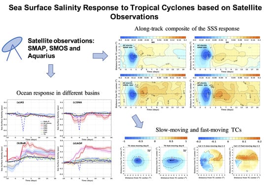
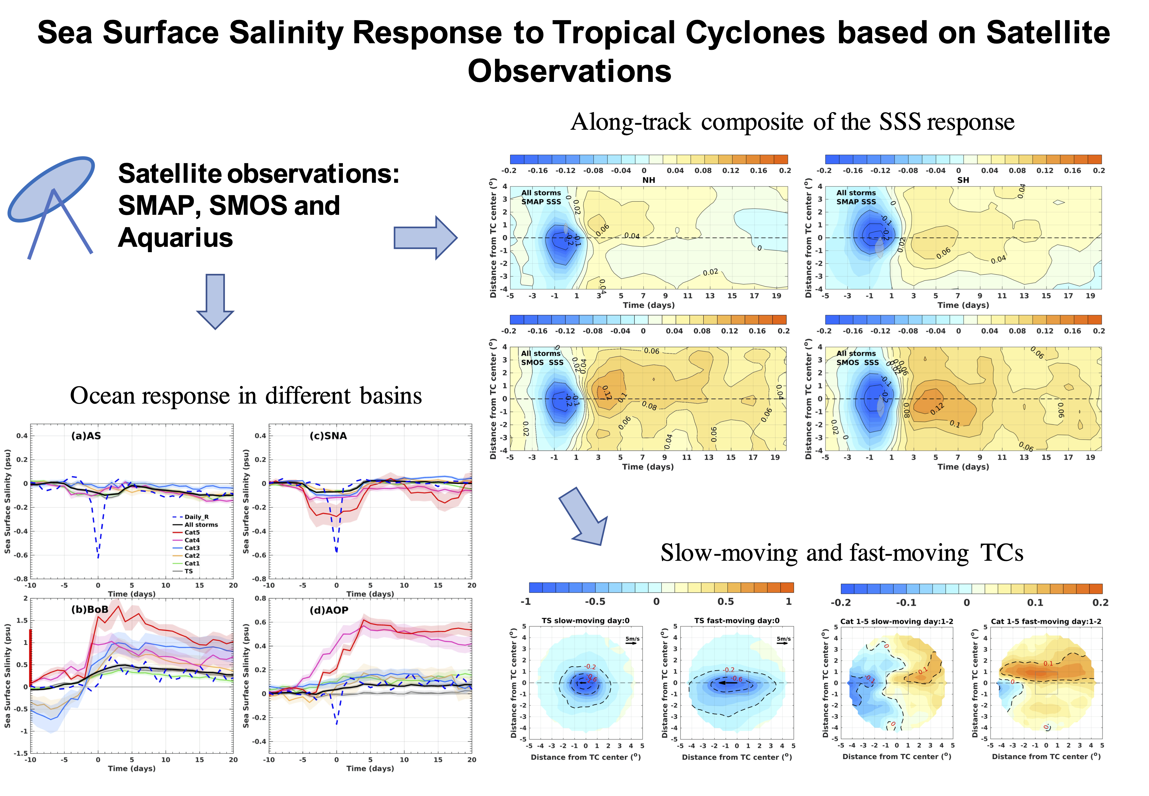
Sea Surface Salinity Response to Tropical Cyclones Based on Satellite Observations

1
Department of Geosciences, Princeton University, Princeton, NJ 08544, USA
2
High Meadows Environmental Institute, Princeton University, Princeton, NJ 08544, USA
3
Atmospheric and Oceanic Sciences Program, Princeton University, Princeton, NJ 08540, USA
4
Rosenstiel School of Marine and Atmospheric Science, University of Miami, Miami, FL 33149, USA
*
Author to whom correspondence should be addressed.
Remote Sens. 2021, 13(3), 420; https://doi.org/10.3390/rs13030420
Submission received: 18 December 2020 / Revised: 15 January 2021 / Accepted: 22 January 2021 / Published: 26 January 2021
(This article belongs to the Special Issue Moving Forward on Remote Sensing of Sea Surface Salinity)

Abstract

:
Multi-year records of satellite remote sensing of sea surface salinity (SSS) provide an opportunity to investigate the climatological characteristics of the SSS response to tropical cyclones (TCs). In this study, the influence of TC winds, rainfall and preexisting ocean stratification on SSS evolution is examined with multiple satellite-based and in-situ data. Global storm-centered composites indicate that TCs act to initially freshen the ocean surface (due to precipitation), and subsequently salinify the surface, largely through vertical ocean processes (mixing and upwelling), although regional hydrography can lead to local departure from this behavior. On average, on the day a TC passes, a strong SSS decrease is observed. The fresh anomaly is subsequently replaced by a net surface salinification, which persists for weeks. This salinification is larger on the right (left)-hand side of the storm motion in the Northern (Southern) Hemisphere, consistent with the location of stronger turbulent mixing. The influence of TC intensity and translation speed on the ocean response is also examined. Despite having greater precipitation, stronger TCs tend to produce longer-lasting, stronger and deeper salinification especially on the right-hand side of the storm motion. Faster moving TCs are found to have slightly weaker freshening with larger area coverage during the passage, but comparable salinification after the passage. The ocean haline response in four basins with different climatological salinity stratification reveals a significant impact of vertical stratification on the salinity response during and after the passage of TCs.

Graphical Abstract

1. Introduction

Tropical cyclones (TCs) are one of the most destructive natural hazards, in terms of human and financial costs. So, understanding the mechanisms behind and improving predictions of TC evolution are of key scientific and societal concern. Due to strong winds and intense heat, momentum and freshwater fluxes, TCs can have a profound impact on the thermal and salinity structure of the upper ocean. These upper ocean changes can feed back onto the evolution of the TC [1,2,3,4,5,6] and may impact the large-scale climate [7]. Therefore, characterizing and understanding the upper ocean response to TCs are important steps for understanding the air-sea interaction during the passage of TCs and consequently the improvement of TC intensity forecasts.
Both observational and modeling studies have shown that TCs drive strong vertical mixing and upwelling, which leads to surface cooling by entrainment of colder subsurface waters [8,9,10,11,12,13]. The TC-induced cooling decreases the heat fluxes from the ocean to the storm, providing a negative feedback with the potential to influence TC intensification [3,4,5,14,15,16]. It has been suggested that subsurface warming driven by TC-induced mixing may impact the mean climate [17,18,19].
Although there is now substantial literature to provide a global perspective on the sea surface temperature (SST) response to TCs and its impact on TC evolution, the interaction between sea surface salinity (SSS) and TCs is less explored. However, studying the surface salinity response provides an additional perspective on the upper-ocean response to TCs, and may be important for understanding the ocean hydrologic cycle and biogeochemical dynamics [20,21,22]. A combined exploration of SSS and SST evolution will provide a more complete understanding of upper ocean dynamics and the ocean density response to TCs.
Because of the sparsity of ocean salinity observations, previous observational analyses have tended to focus on individual case studies. Maneesha et al. [23] found SSS increased up to 0.74 psu on the right of the storm track due to Bay of Bengal (BoB) TC Nargis (2008) with in-situ data. The BoB has the freshest surface and great vertical salinity gradients in the Indian Ocean due to oceanic rainfall and river discharges. A more synoptic view of SSS response to another BoB TC (Vardah 2016) with satellite observations suggests significant increase of SSS (up to 1.5 psu) on the right of the storm and slight decrease on the left [24]. Chaudhuri et al. [25] also reveals the SSS increase of 1.5–3 psu over an area of nearly one million square kilometers after the passage of TC Phailin (2013) in the BoB. Like the BoB, the spreading of the Amazon–Orinoco River plume (AOP) formed a low salinity region in the northwestern tropical Atlantic. Various case studies indicate that the passages of hurricanes in the AOP region can leave a high haline wake with more than 1 psu salinity increase over large areas. However, the SSS change is much weaker outside the plume region [26,27]. Domingues et al. [28] found that the vertical mixing during Hurricane Gonzalo (2014) caused a ~0.6 psu salinity increase in above 20 m and a salinity decrease of 0.4 psu in the layer between 20 and 130 m using underwater gliders situated north of Puerto Rico. The large positive SSS anomaly induced by TCs reflects a strong haline stratification before the passage of TCs. Although these TCs induced large surface salinification, the existence of the strong haline stratification acts as a barrier layer, restricting vertical mixing and amplitude of surface cooling [29,30,31]. A consequence of a strong pre-TC near-surface fresh layer is a reduction of the negative feedback of SST cooling. For example, Androulidakis et al. [32] investigated the interaction between the AOP and three successive hurricanes in 2011. It is found that the existence of a barrier layer during the first storm increased the resistance of the upper ocean to cooling, while the effect was missing in the subsequent two storms as the barrier layer was eroded after the passage of the first hurricane. Observations and model studies have revealed that TC intensification rates can be significantly higher over regions with barrier layers [33,34,35].
In addition to strong vertical mixing and upwelling, intense rainfall and evaporation from the strong TC winds drive surface freshwater fluxes that would act to impact surface and upper-ocean salinity. Although many case studies have revealed a net positive SSS anomaly following a TC, as vertical mixing tends to entrain the subsurface saltier water to the surface, it does not mean that the influence of rainfall on freshening the ocean surface can be neglected. Robertson and Ginis [36] investigated the impact of TC rainfall on ocean salinity with idealized TC forcing and found that the inclusion of rain induced surface negative anomalies in front of the storm center. With underwater gliders, Hsu and Ho [37] found that TCs with heavy rainfall tended to dilute the SSS during TCs, freshening both surface and subsurface. Jourdain et al. [38] found that the positive buoyancy flux due to TC rainfall strengthens the vertical stratification, reduces the vertical mixing and decreases the salty wake left by the passage of a TC. Therefore, TC rainfall acts to reduce the mixed layer depth after the TC passage, hence reducing cold water entrainment [38,39,40]. A slightly fresher mixed layer was observed due to intense rainfall by a moored station south of Kuroshio Extension as typhoon Choi-Wan (2009) was approaching [41]. Kil et al. [42] also found that using satellite data the higher precipitation during Hurricane Isaac (2012) was associated with the lower SSS. A case study designed by Steffen and Bourassa [43] indicates that precipitation by hurricane Gonzalo (2014) produced near-surface freshening of about 0.3 psu and developed a barrier layer during its approach and passage. Lin and Oey [20] reported stronger negative salinity anomalies on the left-hand side of the storms in the western North Pacific because of the leftward asymmetric TC rainfall. Subsurface freshening due to rainfall and vertical mixing is also clearly identified through case and composite studies with in-situ observations [44,45]. As will be shown below, looking across many TCs, the surface salinity response is initially dominated by the TC rainfall and subsequently by vertical ocean processes.
To complement these case studies, we seek to describe the climatological characteristics of the ocean haline response to TCs and compare the salinity changes with the ocean temperature response, through a combined analysis of satellite and in-situ observations. The advent of satellite remote sensing of SSS starting in 2010 opens the possibility to systematically explore the climatology of the SSS response to TCs, with an aim to provide insights into the climatological ocean haline response to TCs that can complement previous case studies (e.g., [24]). Through a series of observational composite analyses, we will describe the response of ocean salinity to TCs, which help elucidate the processes controlling this ocean salinity response. In particular, the present study tries to answer the following questions: 1. What is the typical impact of TC rainfall, evaporation and winds on ocean salinity in terms of climate characteristics? 2. How do TC intensity and translation speed affect the ocean response? 3. What is the difference in ocean response between different basins, and how does it depend on the initial vertical salinity gradients? A recently published paper by Reul et al. [46] characterized the SSS response after TC passage with different methods using 10-year satellite SSS data. The influence of TC intensity, translation speed and vertical salinity gradient on the SSS response during relaxation stage was investigated. Although the SSS response during the forced stage of the TCs and the impact of the balance between precipitation and evaporation are not considered in their study, the climatological SSS response to TCs was studied for the first time at global scale. The consistency and differences between Reul et al. [46] and our study will also be discussed below.
The remainder of this paper is organized as follows. Section 2 introduces data and methods used in the study. Section 3 presents the global averaged ocean salinity response to TCs and evaluates the impact of TC intensity, translation speed, and initial ocean salinification on ocean haline response to TCs. A conclusion and discussion are given in Section 4.

2. Data and Methods

2.1. Data

The center locations and maximum sustained wind speed data of TCs from 2002 to 2019 are obtained from International Best Track Archive for Climate Stewardship (IBTrACS; [47]). TC intensity is defined by 1-minute sustained 10-m wind speed, grouped by TC category on the Saffir-Simpson scale. Supplementary Figure S1 shows the global TC tracks and the intensity category of track positions during the period 2010–2019. The counts of TC track positions for each TC intensity category are present in Table 1. TCs with maximum wind speed of 17 m s−1 or less are excluded. The large-scale wind field from National Center Environmental Prediction (NCEP) daily reanalysis data [48] is used to calculate the vertical wind shear during TCs, which is defined as the difference in wind vectors between 200 and 850 hPa averaged over an annulus region of 200–800 km from the TC center.
Aquarius/SAC-D and Soil Moisture Active-Passive (SMAP) satellite SSS provided by National Aeronautics and Space Administration (NASA) and the European Space Agency’s (ESA) Soil Moisture Ocean Salinity (SMOS) satellite SSS are used to calculate the SSS response to TCs [49,50,51]. The satellite observations have been widely used to investigate the interaction between ocean and TCs (e.g., [25,26,27]). The Aquarius data (version 5.0) covers 2011-08-25 to 2015-06-07 with 150 km spatial resolution. Both level 3 (L3) weekly running mean daily data with horizontal resolution 1° × 1° and level 2 (L2) swath daily data are applied in this study. SMAP satellite data provided by Remote Sensing Systems (version 4.0) are available since 2015-03-27 with a higher resolution (70 km). The SMAP L3 product provides eight-day running meaning daily SSS with horizontal resolution 0.25° × 0.25° while the L2C product contains the validated SSS swath daily data. The L3 eight-day running mean and L2C swath daily data during the period 2015-03-27 to 2019-12-31 are applied in later calculation. We have also included the daily swath data (L2) and ten-day running mean daily data (L3) from SMOS with resolution about 50 km as a complement for our study. The SMOS L2 data obtained from ESA are generated by version 662 of the Level 2 ocean salinity operational processor. The SMOS L3 ten-day running mean data are obtained from Centre Aval de Traitement des Données SMOS (CATDS). The salinity is based on L2Q products, corrected from land-sea contamination and latitudinal bias. SMOS L2 and L3 satellite data from 2010-06-01 to 2019-12-31 are used in this study. For the seven-, eight- or ten-day running daily mean satellite data, the daily SSS is the average between 3, 3.5 or 4.5 days before and after, respectively. SMAP and SMOS satellite data are analyzed to present both the time series and distribution of the SSS response to TCs. However, the Aquarius satellite data are only applied to calculate the time series of the TC related SSS response due to the relatively coarse horizontal resolution.
As we will focus on the ocean surface salinity response during and after the passage of TCs mainly based on satellite observations, the accuracy of satellite SSS retrievals under high surface wind speeds is important to our results. Surface wind is used to estimate the sea surface roughness and its contribution to the brightness temperature during SSS retrievals [52]. However, the surface wind speed used in SSS retrievals is often underestimated for intense TCs, which would therefore make the retrieved SSS less accurate. For example, Meissner et al. [53] indicate that the retrieved SMAP L2C SSS may have moderate degradation when the surface wind speed is larger than 15 m s−1. SSS retrievals are also flagged as moderate degradation when surface wind speed is larger than 15 m s−1 and severe degradation when surface wind speed exceeds 20 m s−1 for Aquarius L2 data. Therefore, to decrease the uncertainty of satellite SSS L3 data, the retrieved L2 SMAP and Aquarius SSS under wind speed higher than 20 m s−1 are discarded during the gridding for the satellite L3 running mean data [53]. The SMOS L2 SSS associated with larger surface wind speed (>12 m s−1) are also removed before averaging to create L3 data due to inaccurate surface roughness for high surface wind speeds. In this study, we will do composite analysis using L2 SSS with and without removing SSS associated with surface wind speed larger than 15 m s−1.
The microwave and infrared (MR_IR) optimally interpolated (OI) SST daily products, provided by the Remote Sensing Systems, from 2010 to 2019 are applied to study the SST response to TCs. Microwave measurements permit retrieval of SST even under overcast conditions and has been widely used in previous studies [4,54,55]. Daily SST observations with 9 km × 9 km are used in this study to calculate the TC related SST change before and after the storm passage. The SST cooling after the TC passage provides a proxy for the TC-induced mixing.
Daily precipitation data are from NASA Global Precipitation Measurement (GPM; [56]) satellite observations with 0.1° horizontal resolution and 0.25° daily evaporation data are obtained by ERA5 reanalysis data [57]. The daily accumulated precipitation and evaporation from 2015 to 2019 are applied to estimate the surface net freshwater flux induced by TCs at daily intervals. In-situ Argo [58] profiles from 2002 to 2019 are also collected during the reference period (pre-storm) and post-storm within the 2° × 2° gridded box centered at a TC position to present the ocean stratification before TCs and the ocean haline response after the TC passage.

2.2. Methods

The SSS, SST, precipitation and evaporation in a 10° × 10° gridded box centered at the TC position from 40 days (day −40) before the TC passed over until 40 days (day 40) after the TC passed are collected. Day 0 indicates the time the TC reaches the position. Every 10° × 10° gridded box is rotated so that the TC translation direction is along the x-axis and pointing to the left. Two examples are shown in Figure 1, where the tracks of hurricane Florence (2018) and Helene (2018) are overlaid on the distribution of SMAP L2C swath daily SSS on 12 September 2018.
The Lagrangian composite method performed to compute the evaluation and distribution of the SSS and SSS response before, during and after the passage of a TC follows that of Lloyd and Vecchi [4]. The SSS and other variables were sampled for a 2° × 2° and 10° × 10° gridded box centered on the TC position (Figure 1). The seasonal cycles were removed to obtain the anomaly for each variable. In order to examine the ocean response to TCs, days −12 to −2 are defined as reference periods for all the satellite swath data, while days −20 to −10 are the reference periods for seven-, eight- or ten-day running mean data. The reference SSS and SST were calculated by averaging the SSS and SST anomaly during the reference period, respectively. The SSS (SST) anomaly relative to the reference SSS (SST) in the same day relative to day 0 were then averaged over all the TC positions to compute the composite SSS and SST anomalies. The composite anomalies were also computed separately by intensity category and translation speed. We define slow (fast)-moving TCs as those with translation speeds half standard deviation smaller (larger) than the group mean TC translation speed. To estimate the uncertainty in the composite mean, standard error is also calculated with s/√n, where s is the sample standard deviation, n is the number of TC track points.

3. Results

3.1. Impact of TC Rainfall and Winds on Ocean Salinity

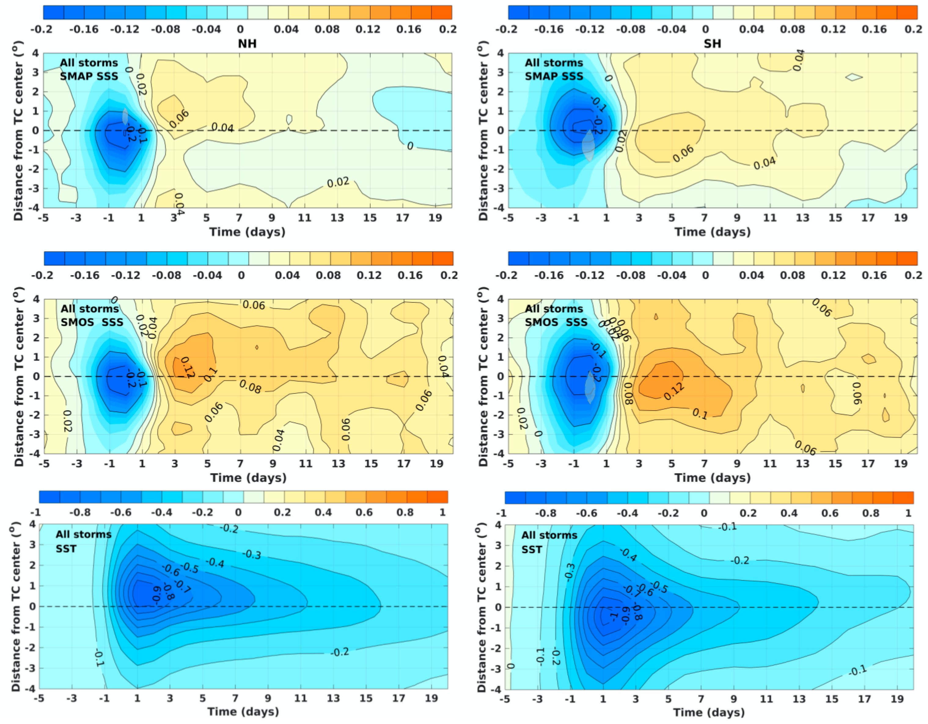
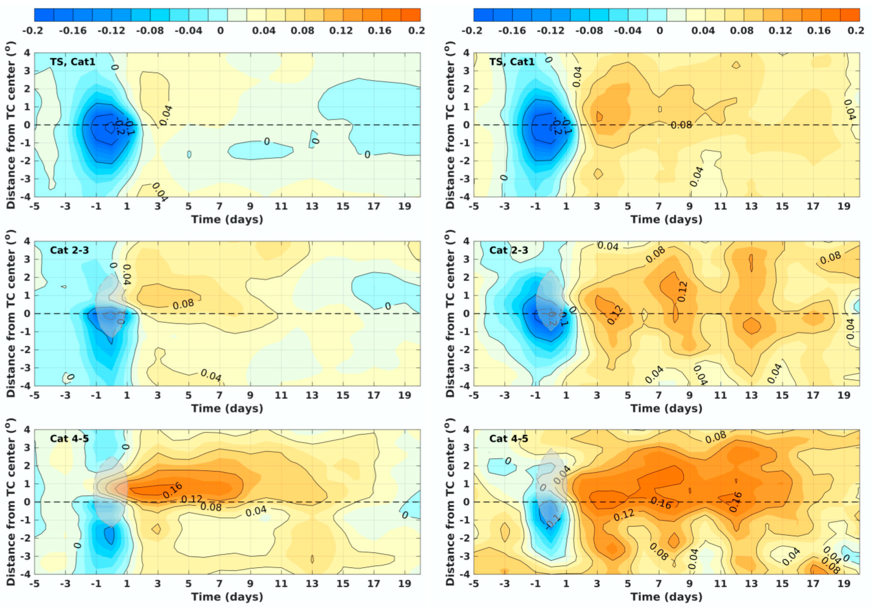
3.1.1. Time Evolution of Ocean Surface Response

Using SMAP swath daily raw data (without removing the SSS associated with high surface wind speeds), the Lagrangian composite SSS anomaly (relative to the reference SSS) shows that on average, as the TC approaches day 0, ocean surface freshens rapidly, with a maximum decrease of mean SSS of more than 0.65 psu (Figure 2b). Freshening varies with TC intensity with a maximum freshening (~0.9 psu) on day 0 for Category 3 TCs (Figure 2a). Due to the degradation of the retrieved SSS under strong surface wind speeds, the SSS response on day 0 has larger uncertainty than in other days, especially for intense TCs; this uncertainty on day 0 will also impact multi-day averages that include it. The impact of the possible contamination of SSS at high wind speeds will be discussed in Section 3.1.2.
The local freshening of the surface lasts approximately one day and is rapidly replaced by a smaller but longer-lasting surface salinification. The largest mean positive SSS response (~0.05 psu) to all storms is observed on day 2. The weaker surface salinification after TCs have passed is observed across the different intensity categories, although the average magnitude of salinification differs. The passage of Category 5 TCs results in the strongest positive SSS response (~0.2 psu) on day 2 and 3 (Figure 2a). The SSS response to different intensity during and after TCs will be further compared in Section 3.2.
The composite SSS response to TCs is also analyzed using SMAP L3 eight-day running mean daily data (Figure 2b). The TC-induced initial freshening and the subsequent salinification are also observed with the smoothed data. Stronger surface salinification after the passage of TCs is clearly evident for intense TCs, although the initial freshening becomes very weak in the smoothed data. As expected, the maximum surface salinification using the L3 eight-day running mean data is observed on day 5, three days later than that calculated with L2C daily data. Despite the delayed response, the magnitude of the positive SSS response is comparable, indicating that the SMAP L3 eight-day running mean SSS data can still capture aspects of the TC-induced SSS response after the storm passage.
Similar behavior is revealed when the analysis above is also applied to Aquarius and SMOS satellite data (Figure 3). On average, the stronger negative SSS response during TCs is followed by weaker but longer-lasting surface salinification after the passage of TCs. The magnitude of the composite mean surface freshening computed with Aquarius swath daily data is 0.25 psu weaker than that of SMAP swath daily data, probably due to the coarse resolution. With similar horizontal resolution, the composite mean surface freshening calculated with SMOS swath daily data is about 0.1 psu larger than that of SMAP data, which may be attributed to different sensors, sampling or data processing of SSS retrievals between these two data products. The reduced salinity response obtained with the seven-/ten-day running mean data on day 0 is also found (Figure 3b,d). Stronger TCs tend to induce larger surface salinification after the passage of TCs, which is consistent with composite analysis results using SMAP data and the results from Reul et al. [46].
The peak in surface freshening on day 0 reflects that the maximum rainfall under a TC is observed on the day the TC passes (day 0; Figure 2c). Figure 2c shows that stronger TCs tend to produce greater precipitation. The daily mean evaporation rate shows similar characters, yet its magnitude only about 10% of the precipitation rate (Supplementary Figure S2). Table 2 compares the values of the daily accumulated precipitation and evaporation on day 0 for different intensity categories, revealing a monotonically increasing relationship between TC intensity and net freshwater flux. Unlike rainfall, the TC induced cooling, which is primarily driven by turbulent mixing and upwelling, reaches its maximum one or two days after a TC has passed (Figure 2d; [4]). The mean SST recovery time after the passage of TCs is more than 20 days for the storms considered here.

3.1.2. Impact of the Possible Contamination of SSS at High Wind Speeds

The composite mean SSS response with SMAP swath daily data after removing the SSS associated with surface wind speed larger than 15 m s−1 is also presented in Figure 2b (dashed blue line). Although surface freshening on day 0 is slightly weaker (~0.05 psu) compared to that with the raw data, the TC related SSS evolution is still characterized with the strong surface freshening and subsequent surface salinification. Similar to SMAP data, after removing the potentially contaminated SSS retrievals due to the high surface winds (>15 m s−1), the SSS negative response on day 0 calculated with Aquarius and SMOS is still evident, with a slightly reduced magnitude (dashed blue lines in Figure 3b,d).
In order to assess the impact of high wind speeds (and their contamination of SSS retrievals) to uncertainty in the SSS response to TCs, the spatial distribution of the percentage of pixels retained from days −1 to 3 for different intensity categories is presented in Supplementary Figures S3 and S4. As expected, more SSS pixels are removed on day 0 compared to days 1 to 3. Also, more SSS pixels are removed during the passage of stronger TCs than with weaker TCs. Therefore, the largest uncertainties of the SSS response to TCs is likely to occur on day 0 for the most intense TCs. The impact of the uncertainty due to SSS retrievals due to high surface wind on tropical storms is likely smaller, with more than 70% of SSS pixels retained in the SSS response to tropical storms on day 0 (Supplementary Figure S3). Therefore, the strong mean negative response on day 0 computed with the high surface wind associated SSS removed satellite L2 data (dashed blue line in Figure 2 and Figure 3) is mainly the average of SSS response to tropical storms. Although significant surface freshening is also observed in relatively intense TCs (Category 1–5) with satellite L2 raw data, the uncertainties arising from stronger wind speeds are more pronounced.

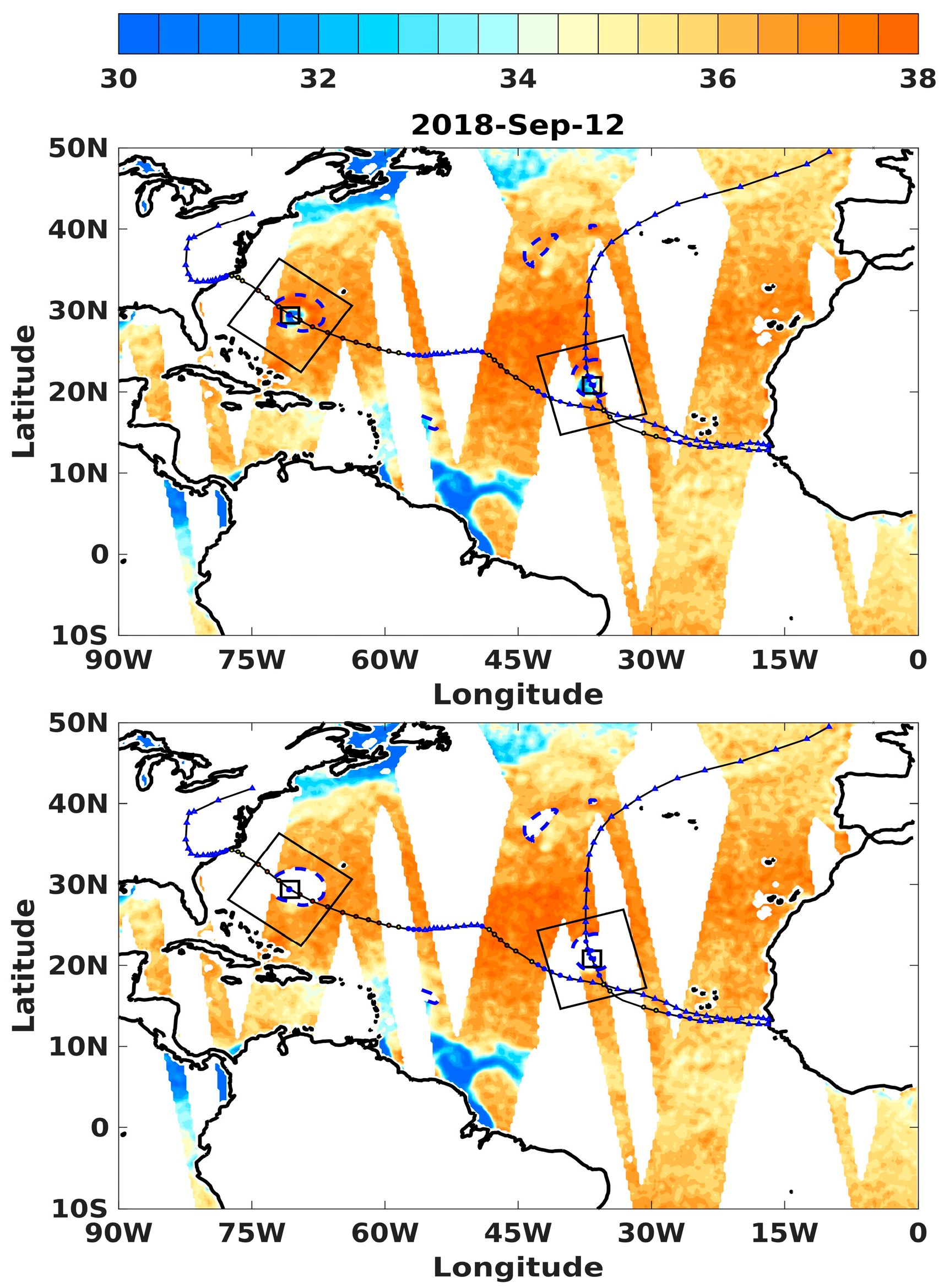
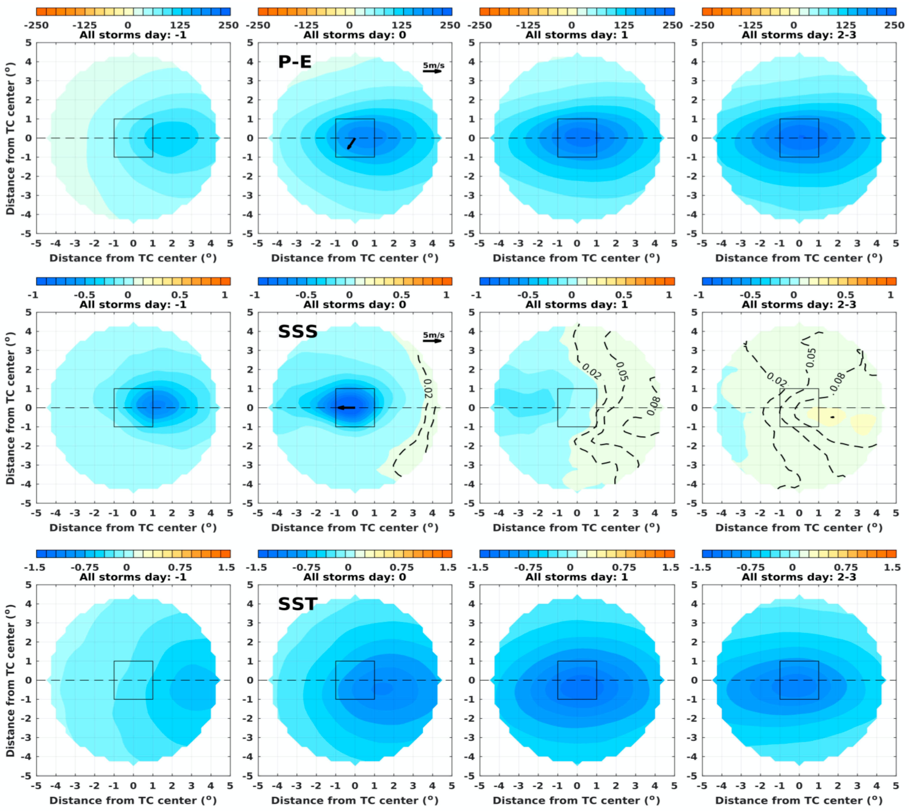
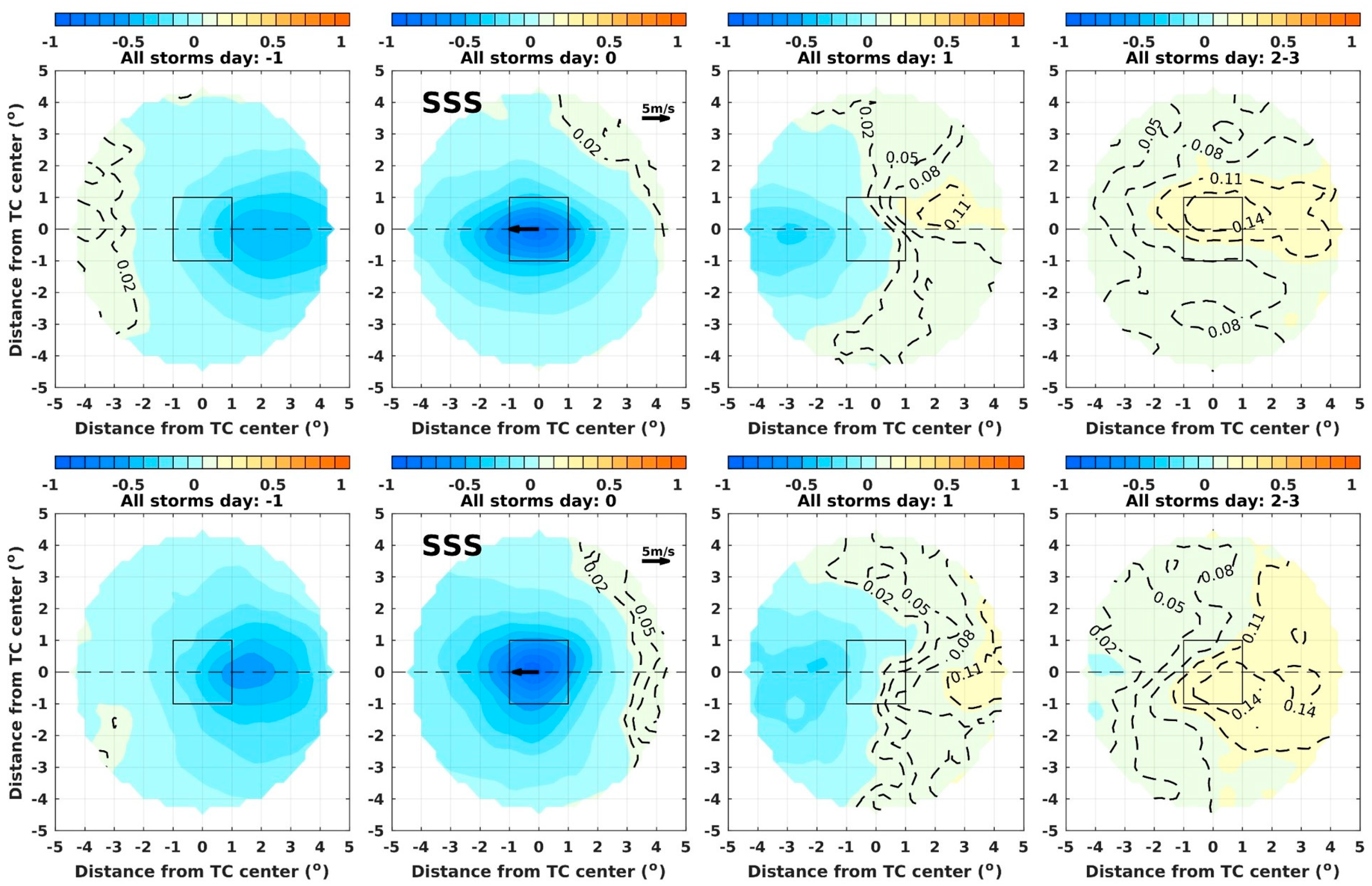
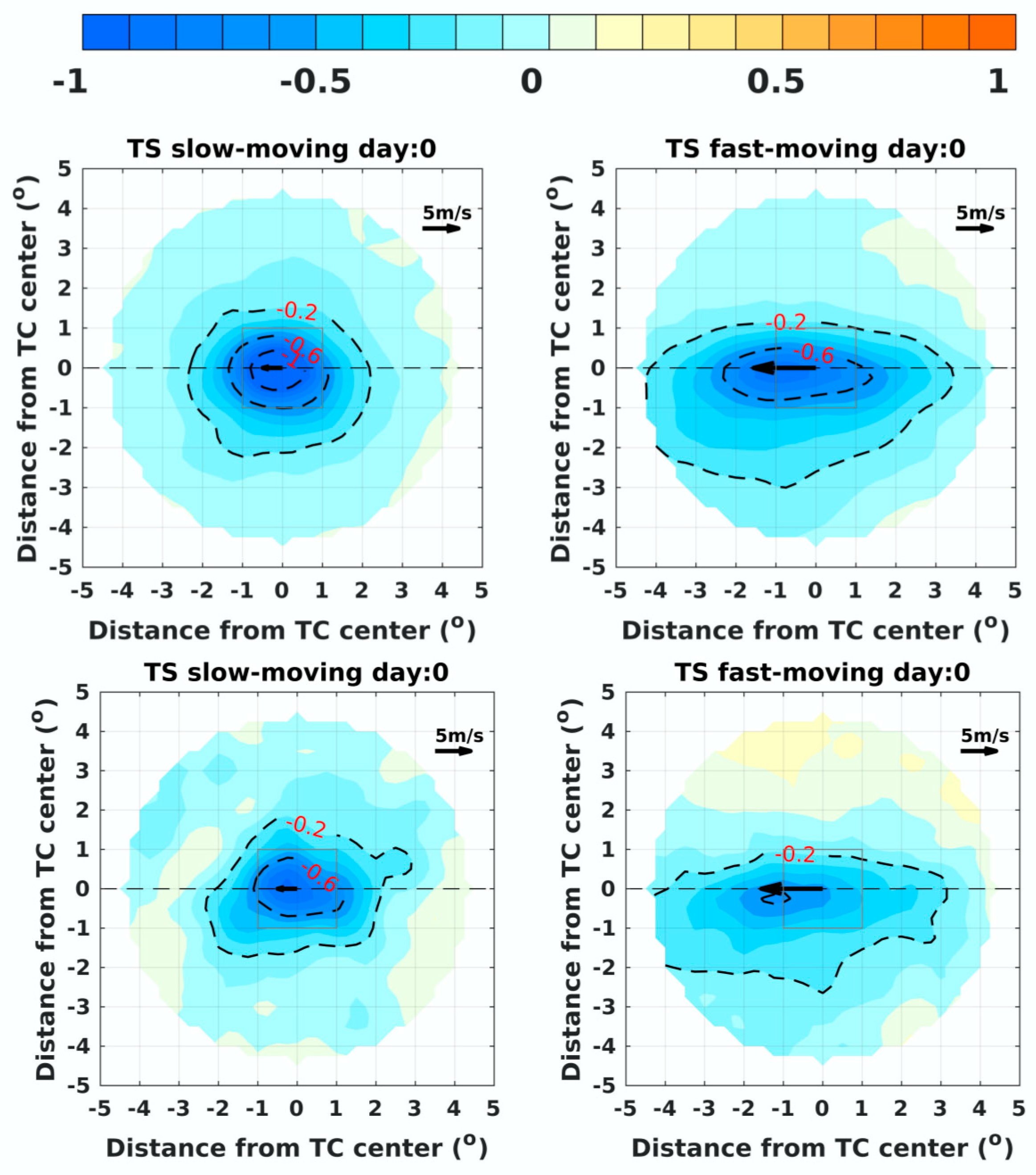
3.1.3. Spatial Distribution of Ocean Surface Response

The spatial distribution of the accumulated precipitation–evaporation (P-E) and SSS (and SST) anomalies relative to reference SSS (and SST) in the Northern Hemisphere from days −1 to 3 are presented in Figure 4. The accumulated P-E is computed starting from day −2. The spatial pattern of accumulated P-E is similar to the pattern of the precipitation since the magnitude of evaporation in the TC center is much smaller than that of precipitation. This is consistent with Gao et al. [59] and indicates a substantial large scale atmospheric convergence of moisture is needed to supply the TC rainfall. The accumulated P-E is distributed symmetrically across the track of the storms. Chen et al. [60] point out that the maximum TC rainfall is on the downshear left (right) side of the storms in the Northern (Southern) Hemisphere when the vertical wind shear is more than 5 m s−1. The composite vertical wind shear on day 0 is only 1.45 m s−1, resulting in a relatively symmetric rainfall pattern; ongoing work explores the dependence on the shear direction of the ocean response to TCs.
The spatial distribution of composited SSS response in Figure 4 is calculated using SMAP L2C swath daily data after removing the SSS associated with the high surface wind. The pattern of SSS response one day before the TCs pass resembles the pattern of P-E, indicating that the net freshwater flux drives the freshening of the ocean surface on day −1. Although more freshwater is accumulated in the rear quadrants of the storms by day 0, the sea surface freshening is concentrated in the center of the TCs. Meanwhile, stronger SST cooling is observed on the rear right quadrant. We hypothesize that the difference between the pattern of P-E and SSS response is caused by the TC-induced vertical mixing.
By days 1 to 3, the spatial pattern of SSS response no longer resembles the pattern of accumulated P-E. After the TC passes, there is an overall tendency towards salinification, resulting in a weaker surface freshening (salinification) is found in the front (rear) quadrants on day 1. The mean surface salinification on days 2–3 shows a pronounced right-hand side bias, which coincides with the stronger right-hand side cooling resulting from TC induced vertical mixing. The TC-induced mixing results in stronger right-hand side cooling and salinification after the passage of TCs in the Northern Hemisphere because on the right-hand side the storm wind vector rotates clockwise, which is in the same sense as inertial current vector, and consequently tends to result in resonance [11,61,62].
The distribution of the composited accumulated P-E, and SST response in the Southern Hemisphere resembles that of the Northern Hemisphere, except that the TC-induced mixing in the Southern Hemisphere is biased to the left of the storm’s tracks (Figure 5). Consistent with our interpretations of the role of mixing on salinification, surface cooling and salinification after the passage of TCs are stronger on the left-hand side, a feature expected due to the resonance between inertial oscillations and wind on the left-hand side. In addition, the mean SSS salinification for the Southern Hemisphere storms on days 2–3 is slightly stronger than that of the Northern Hemisphere storms. The rightward (leftward) peaking surface salinification in the Northern (Southern) Hemisphere is also found by Reul et al. [46], although their post-storm SSS response is averaged from days 0 to 5. They have also pointed that the maximum salinification of the globally-averaged SSS response is at around twice the maximum wind radius. The spatial distribution of SSS response during and after TCs in the Northern and Southern Hemisphere is consistent with the results of composite SSS response evolution shown in Figure 2. The SSS response is initially dominated by the rainfall, leading to a freshening surface. The impact of vertical mixing and upwelling overwhelms rainfall afterwards, offsetting the fresher surface by a longer-lasting salinification through bringing saltier and colder subsurface water to the surface.
The spatial pattern of SSS responses to TCs is also examined with SMOS swath daily data (Figure 6). The SSS associated with the surface wind more than 15 m s−1 is removed. Initial surface freshening on days −1 to 0 and the subsequent salinification in both Northern and Southern Hemisphere are consistent with those seen in the SMAP data. Compared to SMAP, the maximum SSS decrease from SMOS on day 0 is slightly weaker in both Hemispheres. Slightly stronger salinification is also observed on days 1 to 3 with the significant right (left)-hand side biases in the Northern (Southern) Hemisphere. The qualitative consistency between the results with SMAP and SMOS satellite data suggests that the features of the composites represent the actual evolution of SSS following the passage of a TC.
The along-track composite of SSS (SST) response from −4° to +4° to the center between day −5 and day 20 in the Northern and Southern Hemisphere is presented in Figure 7. The SST response is characterized by uniform cooling with the maximum decrease on days 1 to 2. Right (left)-hand side bias is clearly observed in the Northern (Southern) hemisphere, which is consistent with previous studies [11,12,63]. Unlike the SST response, SSS drops primarily during the passage of TCs due to the peak in rainfall. It is worth noting that as the satellite swath SSS pixels under high surface wind are removed, SSS response to relatively intense TCs on day 0 may not be fully considered in the composite calculation. Although TCs produce heavy rainfall, the surface freshening is eventually offset by surface salinification caused by vertical mixing and upwelling, which explains the right (left)-hand side bias distribution of the surface salinification in the Northern (Southern) Hemisphere. Ultimately, the passage of TCs over the ocean results in a cooler and saltier surface, with recovery time more than 15 days. Both SMAP and SMOS satellite data reveal similar SSS response features during and after the passage of TCs, which makes the results more reliable, although the magnitude of the salinification after the passage of TCs is higher when SMOS satellite data are used.

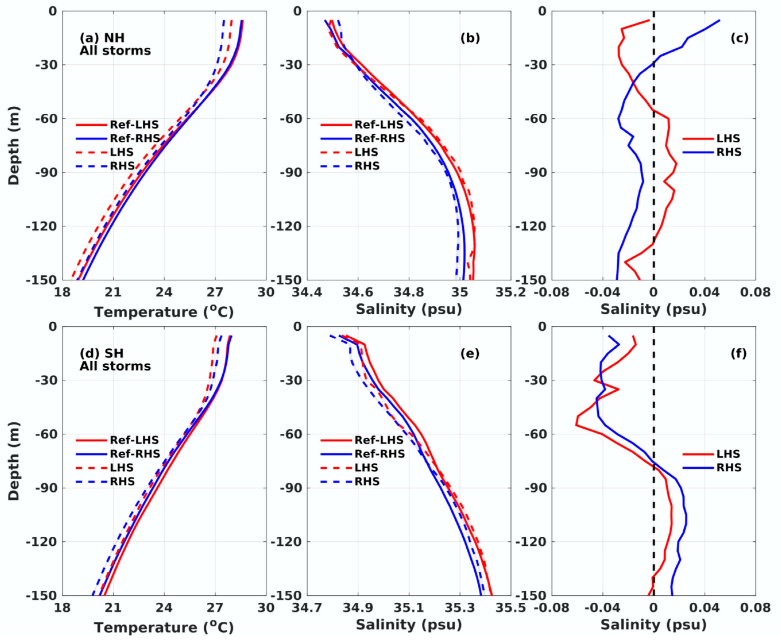
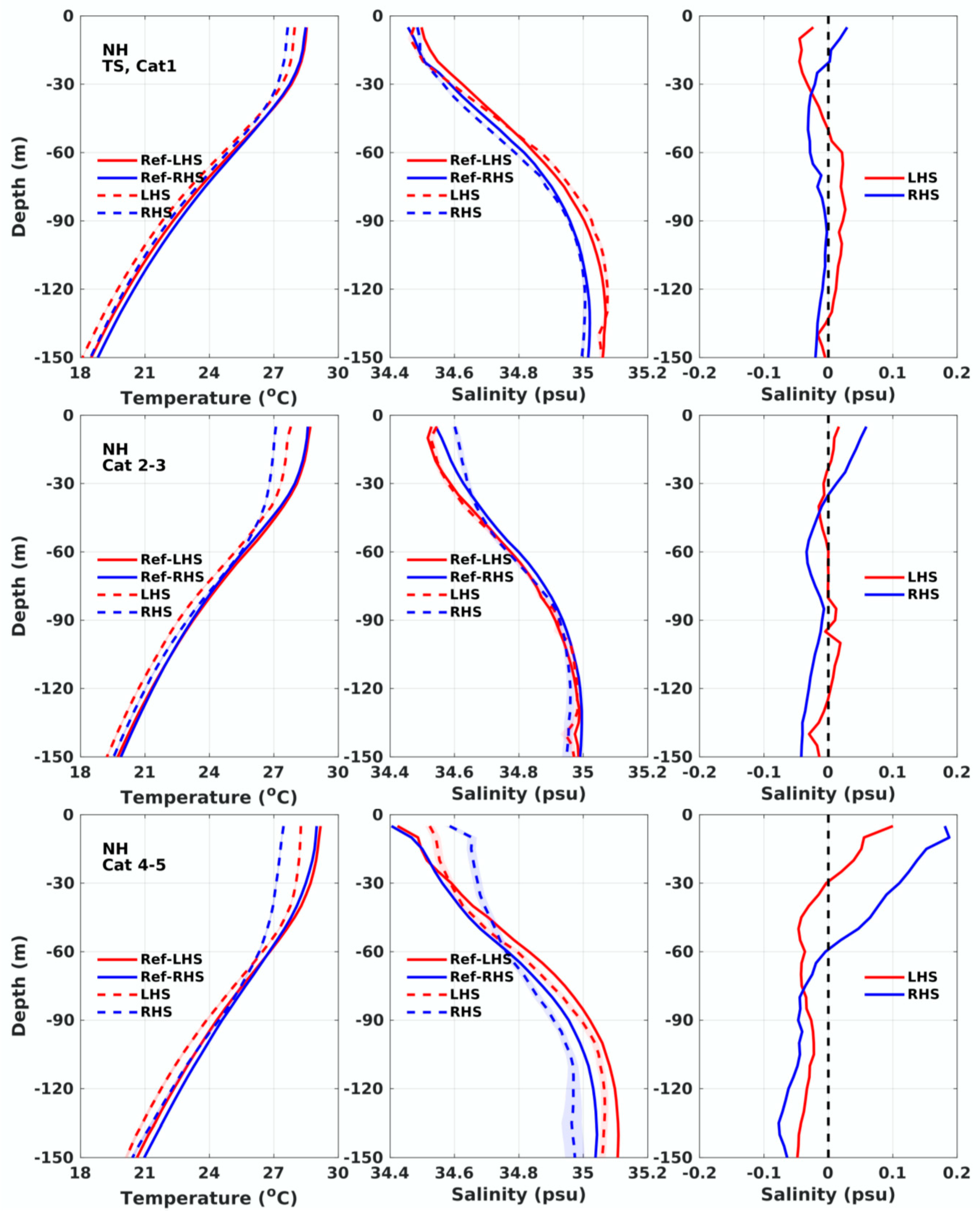
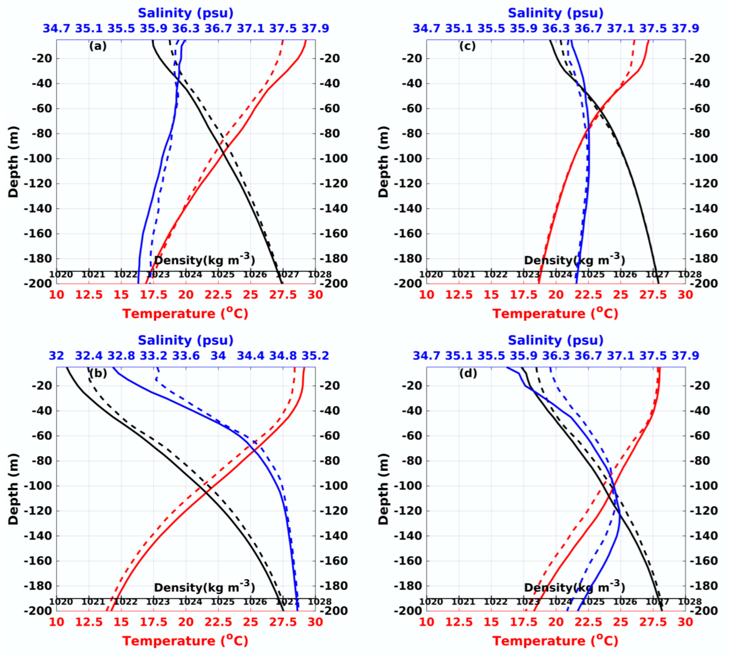
3.1.4. Subsurface Response

The composite vertical stratification with in-situ Argo data during the reference time period (pre-storm) and days 1 to 5 (post-storm) on the right- and left-hand side referenced to the TC heading for both Hemispheres are presented in Figure 8. The salinity (temperature) stratification is defined by the vertical derivation of salinity (temperature), S/z (T/z). Before the passage of TCs, the subsurface water is colder and saltier relative to the surface in both Hemispheres [38]. Therefore, it is expected that the mean vertical stratification of temperature and salinity would result in cooling and salinification, respectively, of the surface from mixing and upwelling (Figure 7). The Argo-derived composite profiles also reveal the subsurface freshening on both sides due to the surface freshwater flux during the TCs. In the Northern Hemisphere, the subsurface freshening on the right (left)-hand side is observed between 30 to 150 m (5 to 55 m) with maximum salinity decrease about 0.03 psu while in the Southern Hemisphere, the subsurface decrease is found in the layer between 5 and 78 m (5 and 76 m) with maximum negative salinity response about 0.06 (0.04) psu on the left (right)-hand side. Stronger and deeper subsurface freshening on the right (left)-hand side is probably attributed to the stronger vertical mixing on the right (left)-hand side in the Northern (Southern) Hemisphere, which could drive more freshwater from the surface to the subsurface.
On average, the passage of TCs is followed by a subsurface salinity increase in the layer between 5 and 30 m on the right-hand side in the Northern Hemisphere. However, the subsurface salinity increase is not found on the left-hand side of the Northern Hemisphere in above 50 m, despite the positive SSS response, indicating that the salinification is confined in the near-surface layer. In the layer between 80 to 150 m in the Southern Hemisphere, we hypothesize that the salinity increase is the result of entrainment and upwelling, which is also observed in the layer between 60 to 130 m on the left-hand side in the Northern Hemisphere. This response, combined with the salinity decrease in the layer between 5 to 80 m, acts to increases the upper ocean density stratification. The ocean haline response to TCs is therefore significantly different from the ocean temperature response: stronger subsurface cooling in above 40 m is followed by weaker cooling in the layer between 40 to 150 m due to turbulent mixing and upwelling, which decreases the ocean stratification (Figure 8a,d). Therefore, the influence of ocean haline response to TCs on the vertical density change after the passage of TCs can be significantly distinct to influence the ocean temperature response due to the existence of surface freshwater flux [64]. Although 11 (5) days of the in-situ Argo profiles are averaged to estimate the pre-storm (post-storm) ocean conditions, the statements above have to be put in light of the poor spatial and temporal sampling of the Argo profiles. The statements can be potentially strengthened by more in-situ observations in the future.

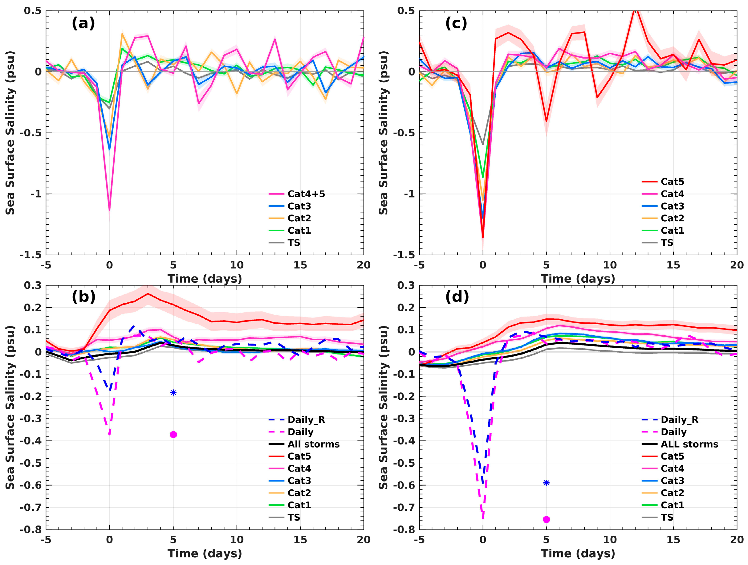
3.2. Influence of TC Intensity and Translation Speed on Ocean Response

To investigate the influence of TC intensity and translation speed on SSS response, the Northern Hemisphere TCs are divided into several groups with different TC intensity categories and translation speeds.

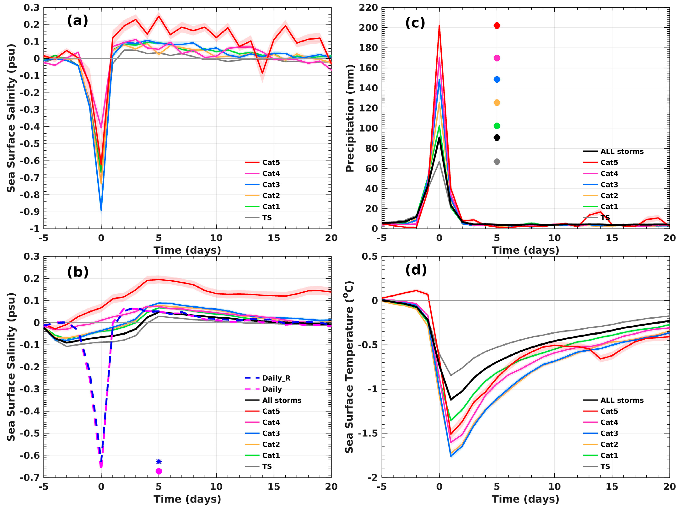
3.2.1. Influence of TC Intensity

The along-track composite of the SSS response from day −5 to day 20 for different intensity categories exhibits similar features with the mean composite of all storms (Figure 9). As the majority of the SSS pixels near the center of relatively intense TCs on day 0 are removed (Supplementary Figure S4), it is difficult to compare the ocean haline response on day 0 to TC-induced precipitation. After the passage of TCs, all TC intensity groups exhibit strong asymmetric surface salinification structure, with the largest positive SSS response on the right-hand side of the storms in the Northern Hemisphere. It is also found that intense TCs tend to drive stronger and longer-lasting surface salinification. The along track ±4° composite with SMAP swath data shows that TS and Category 1 TCs result in mean SSS increase of more than 0.04 psu on the right-hand side of the storms during days 2 to 4. The positive SSS response then slightly decreases. However, the ocean surface response remained positive until day 14. The maximum positive SSS response to Category 2–3 (Category 4–5) TCs reaches more than 0.06 (0.12) psu from days 2 to 8. The positive salinity response of larger than 0.04 psu is maintained until 10 (17) days after the passage of TCs for Category 2–3 (Category 4–5) TCs. When SMOS swath data are used, a similar phenomenon is observed, although the SSS positive response is systematically stronger than that calculated with SMAP data. Both data indicate that although stronger TCs tend to produce more precipitation and consequently input more freshwater into the ocean, the surface freshening is eventually overwhelmed by the more intense vertical mixing. Thus, stronger TCs ultimately induce a saltier surface with a longer recovery time. Consistent with our findings, Reul et al. [46] have also found that more intense storms tend to produce saltier globally-averaged SSS response on days 0 to 5.
The vertical structure under the TC center for different intensity groups is compared using Argo in-situ data (Figure 10). Consistent with the composite of the Argo-derived vertical profiles before the passage of all storms (Figure 8), colder and saltier subsurface water is found for all TC intensity groups on both sides of the storms. The passage of TCs generally results in stronger subsurface cooling above 30 to 60 m and weaker subsurface cooling deeper than that. All the intensity groups exhibit stronger upper layer cooling on the right-hand side.
The ocean haline response shows different features. For group TS and Category 1, although the surface salinification is presented on both sides after the TCs overpass (Figure 9), the subsurface upper layer (the above 30 m) salinification is only found on the right-hand side due to stronger vertical mixing. On the left-hand side, the subsurface layer from 5 m to about 50 m displays a weaker salinity decrease, indicating that the surface salinification exists in a very shallow near-surface layer on the left-hand side. For Category 2–3 and Category 4–5, both sides manifest subsurface upper layer salinification with a larger salinity increase and a deeper upper layer on the right-hand side. For all the intensity groups, below the upper salinification layer, the freshwater flux during the TCs results in a layer of salinity decrease, with greater freshening on the right-hand side. Therefore, compared to the right-hand side, both the temperature and salinity response to TCs lead to a stronger stratification on the left-hand side in the Northern Hemisphere.

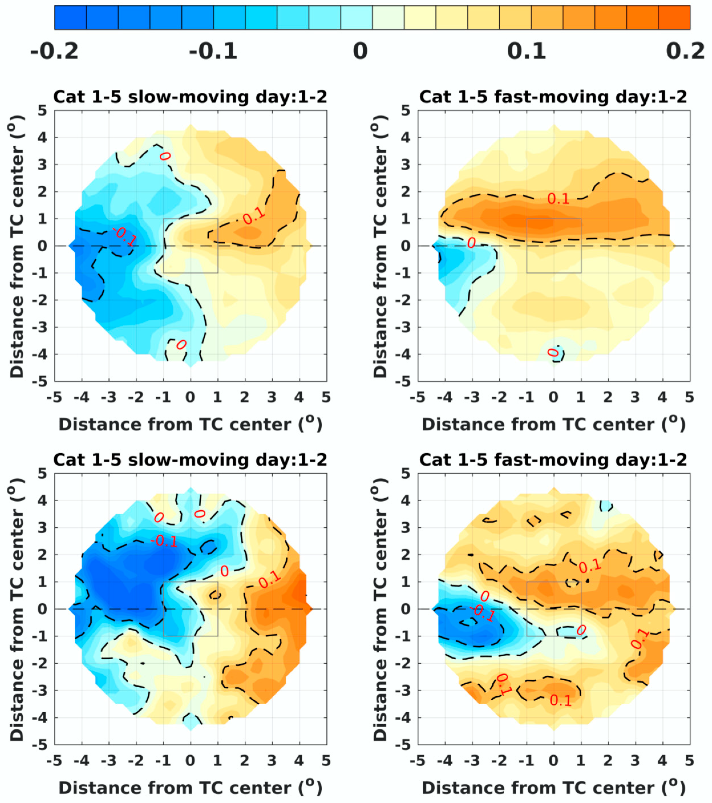
3.2.2. Influence of TC Translation Speed

We further explored the influence of TC translation speed on surface salinity response. Slow-moving TCs could increase the amount of TC-related daily accumulated rainfall and consequently result in stronger freshwater flux (Supplementary Figure S5). In addition, slow-moving TCs also tend to input more momentum flux into the ocean, leading to enhanced vertical mixing and SST cooling [65,66]. The composites of SSS response to tropical storms on day 0 in two groups of translation speed (see Method) are shown in Figure 11. The mean translation speed of slower and faster cases is 2.48 m s−1 and 7.80 m s−1, respectively.
To compare the ocean haline response to different translation speed on day 0, SSS response to tropical storms is used because more SSS pixels are retained for tropical storms (Supplementary Figure S3). The degradation of SSS retrievals under high wind speeds makes it hard to compare the SSS response on day 0 to relatively intense TCs. The SMAP satellite data show that the surface freshening induced by slow-moving tropical storms covers a smaller area and concentrates near the composite center of the tropical storms, while the surface freshening for fast-moving tropical storms covers a much larger area with the maximum decrease (~0.6 psu) weaker than that (~1 psu) of the slow-moving groups. Similar results are noted with SMOS satellite data, indicating that fast (slow)-moving tropical storms tend to result in a weaker (stronger) surface freshening with larger (smaller) area coverage.
After the passage of TCs, the positive SSS response on days 1–2 for slower storms is concentrated near the center and rear quadrants, while greater negative SSS response is observed in the front quadrants (Supplementary Figure S6 and Figure 12). As more freshwater is accumulated for slower cases (Supplementary Figure S5), the salinity stratification is enhanced, which inhibits the vertical mixing and surface salinification. Compared to slower cases, faster-moving TCs lead to weaker negative SSS anomalies with smaller area coverage in the front quadrants because of the less freshwater accumulation. Although slower-moving TCs tend to have larger momentum and evaporative fluxes and induce cooler SST, the value of the maximum positive SSS response is comparable to the faster-moving TCs, as there is more freshwater accumulated and stronger surface freshening during TCs, offsetting the effect of enhanced evaporation and mixing.

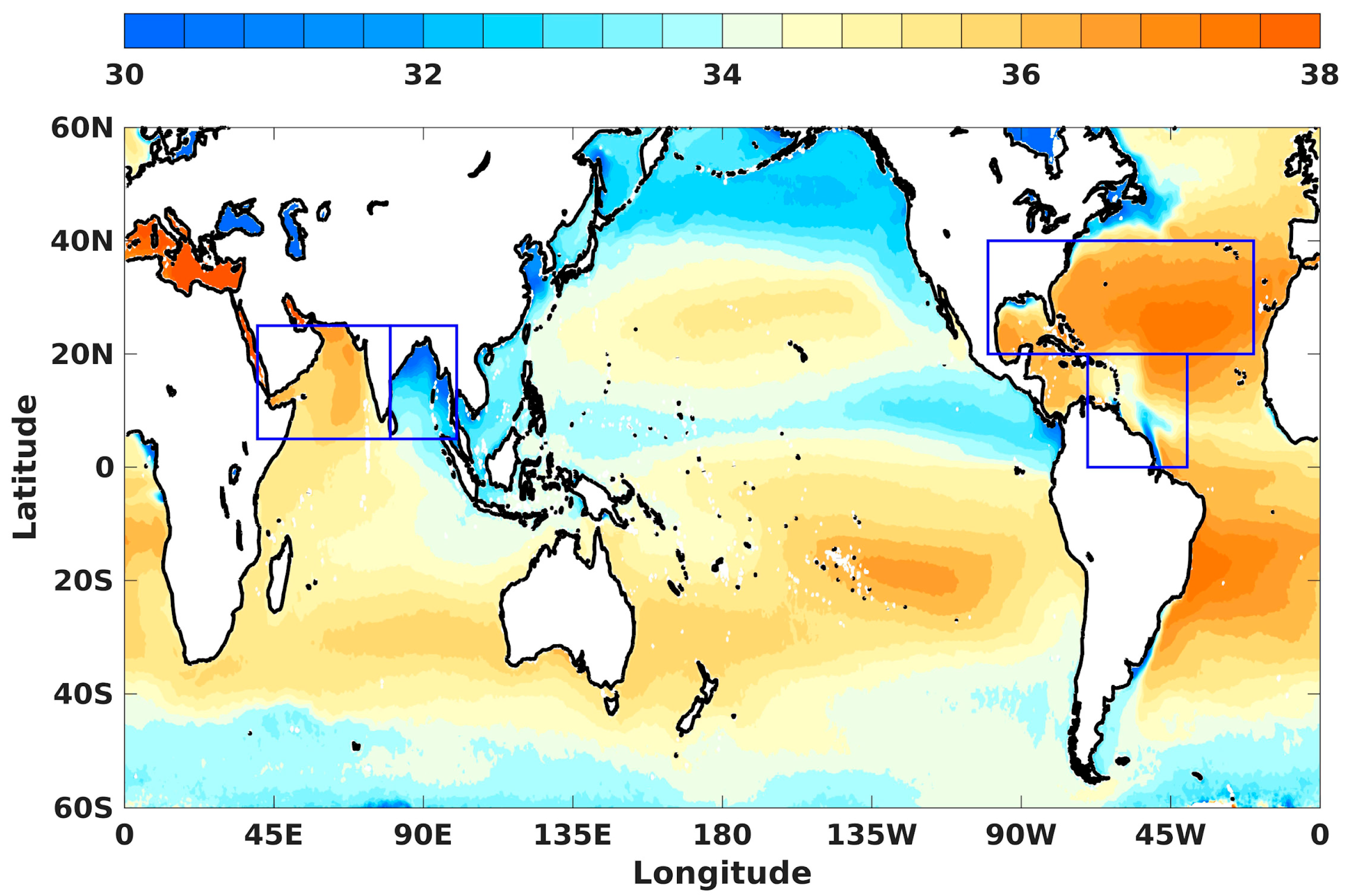
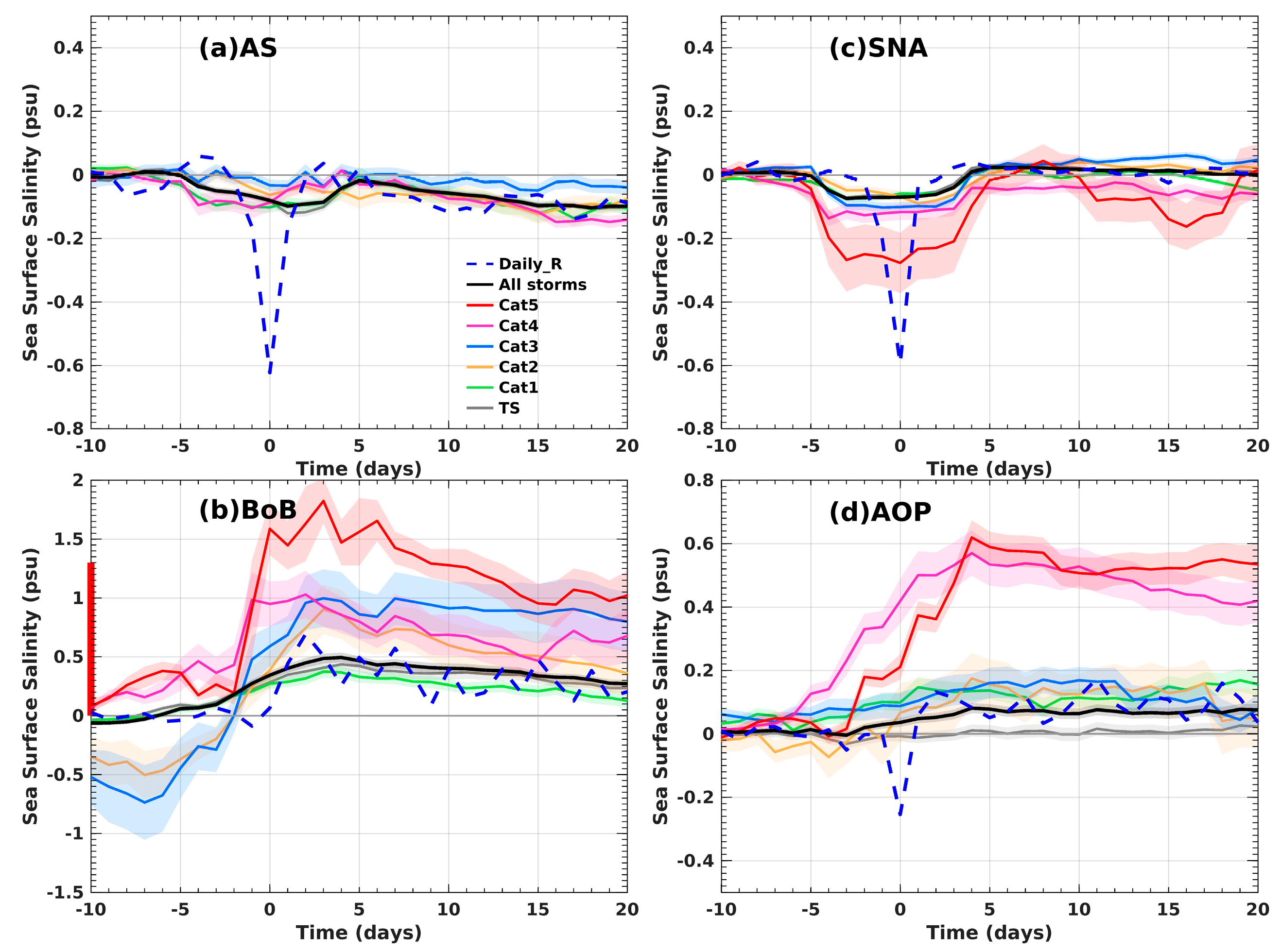
3.3. Ocean Response in Different Basins

The mean ocean tropical salinity and temperature stratification is characterized with fresher and warmer surface water and saltier and cooler subsurface water in both Northern and Southern Hemisphere during the reference period (Figure 8). However, the surface salinity and salinity stratification differ markedly between different basins, and we choose four basins to investigate and illustrate the influence of background salinity and temperature stratification on ocean response to TCs (Figure 13). The Arabian Sea (AS) and the Bay of Bengal (BoB) are two basins in the northern Indian Ocean, each with distinct surface salinity and salinity stratification. The BoB is one of the freshest regions in tropics as a result of oceanic rainfall and river runoff. Compared to the BoB, the AS SSS is higher mainly due to enhanced evaporation and vertical mixing of surface water with subsurface water [67]. The Atlantic presents two other contrasting subbasins. The Subtropical North Atlantic (SNA) exhibits the highest SSS values worldwide with mean SSS exceeding 37 psu [68,69]. Lower surface salinity in the Amazon–Orinoco Plume (AOP) region is attributed to the spreading of freshwater plumes from the Amazon and Orinoco River.
Figure 14 compares the Argo-derived temperature, salinity, and density stratification before the passage of TCs during the reference time period in four regions. BoB and AOP display greater salinity and density stratification, resulting in an approximately 20–30 m mean barrier layer, while the ocean preconditions in the AS and SNA are characterized by weaker stratification and higher surface salinity. On average, the subsurface water in the SNA (AS) is slightly saltier (fresher) than the surface.
The composite evolution of SSS anomalies for each of the four basins are presented in Figure 15. To obtain more samples, both Aquarius and SMAP satellite data are used (Figure 15). The SSS response time series for these four basins calculated with SMOS satellite data (Supplementary Figure S7) shows similar features. The SSS anomaly calculated with satellite swath daily data exhibits great surface freshening on day 0 in both AS and SNA but much smaller freshening in the AOP. The initial surface freshening due to precipitation is not obvious during the passage of TCs in the BoB. As the SSS under high surface wind is removed from the swath daily data, the surface response on day 0 to intense TCs may not be well displayed. Because of the small sample size in each basin, the Aquarius and SMAP seven-/eight-day running mean data (Figure 15) and SMOS ten-day running mean data (Supplementary Figure S7) are applied to investigate the SSS response to different intensity categories after TCs overpass. It is found that the TC-induced mixing produces a weaker positive response even for intense TCs due to weaker salinity stratification in the SNA. The composite SSS response after TC passage is negative in the AS because of the fresher subsurface salinity (Figure 14), thus TCs in the AS eventually result in a fresher surface. In contrast, TCs in the BoB lead to strong surface salinification. Note that the y-axis of Figure 15b is modified to −1.5 to 2 psu (−1.5 to 3 psu in Supplementary Figure S7b). The mean salinification reaches the maximum on day 2 with the positive SSS response exceeding 0.5 psu, 10 times of the global mean SSS response on day 2. Relatively intense TCs (Category 3–5) in the BoB caused extremely large surface salinification. The amplitude of the positive SSS response after the passage of TCs is as high as 1.5 psu for Category 5 TCs, consistent with the dependence of SSS response amplitude to TCs on vertical salinity gradients and storm intensity shown in Reul et al. (their Figure 3c, [46]). The mean salinification after the passage of TCs in AOP is approximately 0.1 psu, two times of the global mean. However, Category 4–5 TCs exhibit much higher surface salinification (~0.6 psu) than the mean salinification in AOP, which is consistent with the case studies mentioned in the introduction. A possible interpretation is that the most intense TCs (Category 4–5) tend to develop after a strong river plume, and we hypothesize that fresher surface results in stronger vertical stratification, reduces the SST cooling, and facilitates the TC intensification.
The along-track composite of SSS response during and after the passage of TCs are compared in Figure 16. The distribution of the along-track SSS response in the SNA is similar to the mean SSS response to all storms in the Northern Hemisphere (Figure 7). However, the surface response in the AS shows a notably different pattern: the stronger surface freshening on day 0 is followed with weaker surface freshening after the passage of TCs. As a result of the higher surface salinity, the vertical mixing induces subsurface salinification in the AS after the passage of TCs (Figure 14a). The subsurface response in the AS is therefore distinct from the subsurface response in the SNA (Figure 14c) and the composite mean subsurface response in the Northern Hemisphere (Figure 8), where strong mixing brings surface freshwater to the subsurface, and reduces the subsurface salinity.
It is also confirmed in Figure 16 that the surface salinity response to TCs in the SNA and AS is much weaker than that of the BoB and AOP, as would be expected from the weaker salinity stratification in the SNA and AS basins. In the BoB and AOP, entrainment acting on the strong salinity stratification makes the initial surface freshening weaker but is conducive to substantial salinification of the sea surface after TCs pass. The asymmetric pattern for the average response is also remarkable. The SSS positive response spans over a large area and mainly on the right-hand side of storm motion in BoB and AOP. Besides the surface salinification, subsurface salinification is also significant in the upper 80 m owing to the strong salinity stratification in these two basins (Figure 14b,d).

4. Discussion and Conclusions

In this study, the spatial and temporal signatures of ocean salinity response to TCs are investigated with Aquarius, SMAP, and SMOS satellite SSS data and in-situ Argo profiles, which show distinct characteristics from the ocean temperature response. The storm-following composites of ocean haline response are also analyzed for different TC intensity, translation speed, and basins.
On average, as a TC passes over a position, rapid surface cooling is induced with maximum SST response reaching one or two days after the TC passes ([4,5]; Figure 2 and Figure 7). The passage of TCs produces a cold wake that is enhanced to the right (left) of 2storm motion in the Northern (Southern) Hemisphere, and the recovery time is more than 20 days. Typically, strong winds cause a negative air-sea enthalpy flux and drive the cold water from below entrain into the mixed layer, cooling the surface. In addition, TC rainfall may also lead to surface cooling as rainfall is often colder than the surface ocean. Previous studies estimated a no more than 10% contribution of surface heat loss by TC rainfall [70,71].
The response of the SSS to TCs exhibits significantly different features from the SST response. Our results show that the SSS response to TCs is initially dominated by the TC induced rainfall and subsequently controlled by wind driven vertical mixing and upwelling. The dominance of precipitation over evaporation in the net salinity budget near the storm indicates that much of the atmospheric moisture necessary to sustain the storm rainfall is evaporated at a distance of at least several hundred kilometers away from the storm center. On average, SSS decreases significantly on day 0 due to the net surface freshwater flux (positive P-E), with negative SSS anomaly averaged over the TC-centered 2° box more than 0.60 psu when SMAP swath data are used. Strong surface freshening is followed by weaker and longer-lasting surface salinification after the passage of TCs. Vertical mixing and upwelling act to entrain the saltier subsurface water, leaving behind a right (left) biased wake of higher SSS in the Northern (Southern) Hemisphere with recovery time more than 15 days after the passage of TCs, as the storm wind vector on the right (left)-hand side rotates clockwise (anticlockwise) in the same sense as the inertial oscillation. With combined SMAP and SMOS satellite data, Reul et al. [46] also found that the passing hurricanes induced surface salinification with maximum positive anomaly on the right (left)-hand side in the Northern (Southern) Hemisphere at around twice the maximum wind radius. The comparable recovery time of SSS and SST is somewhat perplexing since surface heat fluxes would tend to damp SST anomalies, but net surface salinity fluxes are not fundamentally dependent on background salinity. The mechanisms for the relaxation of the storm induced SSS signal merit further exploration.
The Argo-derived composite profiles reveal that the ocean temperature response to TCs is characterized by stronger subsurface cooling in above 40 m and weaker cooling in the layer below, which would act to decrease ocean temperature and density stratification. However, subsurface freshening is observed on both sides of storms with stronger and deeper freshening on the right (left)-hand side in the Northern (Southern) Hemisphere. The ocean haline response on TCs may therefore act to increase the vertical density stratification.
The influence of TC intensity and translation speed on the surface response is also examined by dividing the Northern Hemisphere TCs into different groups. Although more intense TCs tend to input more freshwater flux into the ocean, the surface negative response of different intensity categories is eventually replaced by the surface salinification. It is found that longer-lasting and greater surface salinification is induced by stronger TCs due to stronger vertical mixing and upwelling. The saltier surface response for more intense TCs is also presented by Reul et al. [46]. It is distinct from the nonmonotonic SST response to different intensity categories: maximum cooling is observed in Category 3 TCs as extreme TCs tend to occur in the ocean with weaker upper-ocean stratification and larger ocean heat content (Figure 2d; [4,5]). Besides stronger surface salinification, stronger TCs account for the larger and deeper subsurface upper layer salinity increase, especially on the right-hand side of storm motion in the Northern Hemisphere.
As to the ocean response to TCs with different translation speed, satellite observations indicate stronger (weaker) surface freshening during TCs but comparable surface salinification on days 1–2 after the passage of TCs for slow (fast)-moving TCs due to the negative effect of the TC-induced rainfall on vertical mixing. However, surface cooling after the passage of TCs tends to be larger for slow-moving than fast-moving TCs (e.g., Figure 2, [4]). Reul et al. [46] investigated the averaged SSS response on days 0–5 to TCs with different translation speed. The nondimensional storm translation speed τ is used in their study, which is defined by the ratio of local inertial period to the TC residence time. The surface salinification for TCs with smaller τ (τ < 1) is found two times larger than that of larger τ (τ > 1) because of the longer storm residence and stronger vertical mixing [4].
The ocean response in four illustrative basins with different ocean climatological salinity stratification are compared. Strong salinity stratification enhances the positive SSS response following the passage of a TC in the BoB and AOP region. In contrast, the weaker salinity stratification in the AS and SNA results in a more muted response of salinity after the TC passage and a greater tendency for freshening during the TC. Previous case studies have found similar results to these composite analyses. For example, Grodsky et al. [26] found that the passage of Hurricane Katia (2011) resulted in a 1.5 psu positive salinity wake with weekly averaged Aquarius and SMOS satellite data in the AOP region. Based on ten-day averaged SMOS satellite data, a similarly strong surface salinification was also observed after Hurricane Igor (2011) in the AOP region [27]. Chacko [24] reported that BoB TC Vardah (2016) induced a significant increase of SSS (up to 1.5 psu) on the right of the storm with eight-day running SMAP data. These results are consistent with the composite salinity response to TCs in the AOP and the BoB region, in which the ocean response is characterized by strong positive salinity anomaly while surface freshening is hardly observed. Reul et al. [46] have also found that the vertical salinity stratification before TCs significantly contributes to the regional variability of SSS response to TCs. Consistent with our study, striking surface salinification is found in the BoB and AOP region due to the fresh surface river plume and stronger vertical salinity stratification. Besides BoB and AOP, river plume regions of Mississippi, Pearl, and Yangtze are also characterized with strong salinification after the passage of TCs. On the contrary, in the AS and SNA the mean SSS response is dominated by surface freshening on days 0–5. The negative surface response after the TC passage in the AS is consistent with our results. In the SNA, our results show striking surface freshening on day 0 and very weak surface salinification during days 2–8. Both the results in our study and that of Reul et al. [46] emphasize the significant dependency of ocean salinity response on the pre-storm ocean salinity stratification.

Supplementary Materials

The following are available online at https://www.mdpi.com/2072-4292/13/3/420/s1, Figure S1: Global TC tracks during the period 2010–2019, from IBTrACS data. Colors indicate the TC category based on the Saffir-Simpson scale from Tropical Depression to Category 5. Figure S2: Lagrangian composite of daily accumulated evaporation during the same period with Figure 2, from ERA5. Figure S3: The percentage of the SSS pixels retained for TS, Category 1 and Category 2 TCs after removing the SSS associated with the surface wind speed higher than 15 m s−1 from the SMAP L2 swath daily data. Figure S4: The percentage of the SSS pixels retained for Categories 3 to 5 TCs after removing the SSS associated with the surface wind speed higher than 15 m s−1 from the SMAP L2 swath daily data. Figure S5: Distribution of daily accumulated P-E (mm) on day 0 in the Northern Hemisphere based on translation speed during the same time period with Figure 11. The mean translation speed in upper (lower) panels is 2.48 (2.67) and 7.80 (7.44) m s−1, respectively. Figure S6: Distribution of SSS response (psu) to tropical storms on days 1–2 based on translation speed in the Northern Hemisphere, with SMAP (upper panels) and SMOS (lower panels) swath daily data. Same time period with Figure 12 is used for both SMAP and SMOS satellite data. Figure S7: The same with Figure 15, but with SMOS satellite data. The range of y-axis is 1.3 psu for (a), (c) and (d) while 4.5 psu for (b).

Author Contributions

Conceptualization, J.S. and G.V.; methodology, J.S., G.V. and B.S.; validation, J.S., G.V. and B.S.; formal analysis, J.S.; writing—original draft preparation, J.S.; writing—review and editing, J.S., G.V. and B.S.; visualization, J.S.; project administration, G.V.; funding acquisition, G.V. All authors have read and agreed to the published version of the manuscript.

Funding

This work was funded in part by Award 80NSSC19K0482 from the National Aeronautics and Space Administration and by the Carbon Mitigation Initiative at Princeton University.

Institutional Review Board Statement

Not applicable.

Informed Consent Statement

Not applicable.

Data Availability Statement

All Aquarius and SMAP satellite data created or used during this study are openly available from Physical Oceanography Distributed Active Archive Center at https://podaac.jpl.nasa.gov/datasetlist. SMOS satellite salinity data used during this study are openly available from ESA SMOS Online Dissemination Service at https://smos-diss.eo.esa.int/smos/faq.html. OISST used in this study is openly available from http://www.remss.com/measurements/sea-surface-temperature/. NCEP reanalysis data used in this study are openly available from NOAA Physical Sciences Laboratory at https://psl.noaa.gov/data/gridded/data.ncep.reanalysis.html. GPM precipitation data used in this study are openly available from https://disc.gsfc.nasa.gov/datasets/GPM_3IMERGDF_06/summary. ERA5 evaporation data used during this study are openly available from Copernicus Climate Change Service at https://www.ecmwf.int/en/forecasts/datasets/reanalysis-datasets/era5. Argo in-situ data used in this study are openly available from North Carolina Government Data Analytics Center at ftp://ftp.ifremer.fr/ifremer/argo.

Acknowledgments

The authors want to thank all the satellite groups participating in Aquarius, SMAP, SMOS, etc. for producing and sharing the satellite remote sensing data.

Conflicts of Interest

The authors declare no conflict of interest.

References

  1. Emanuel, K.; DesAutels, C.; Holloway, C.; Korty, R. Environmental control of tropical cyclone intensity. J. Atmos. Sci. 2004, 61, 843–858. [Google Scholar] [CrossRef]
  2. Jacob, S.D.; Shay, L.K. The role of oceanic mesoscale features on the tropical cyclone–induced mixed layer response: A case study. J. Phys. Oceanogr. 2003, 33, 649–676. [Google Scholar] [CrossRef]
  3. Kaplan, J.; DeMaria, M. Large-scale characteristics of rapidly intensifying tropical cyclones in the North Atlantic basin. Weather Forecast. 2003, 18, 1093–1108. [Google Scholar] [CrossRef] [Green Version]
  4. Lloyd, I.D.; Vecchi, G.A. Observational evidence for oceanic controls on hurricane intensity. J. Clim. 2011, 24, 1138–1153. [Google Scholar] [CrossRef]
  5. Lloyd, I.D.; Marchok, T.; Vecchi, G.A. Diagnostics comparing sea surface temperature feedbacks from operational hurricane forecasts to observations. J. Adv. Model. Earth Syst. 2011, 3, M11002. [Google Scholar] [CrossRef]
  6. Sun, J.; Oey, L.-Y. The Influence of the Ocean on Typhoon Nuri (2008). Mon. Weather Rev. 2015, 143, 4493–4513. [Google Scholar] [CrossRef]
  7. Emanuel, K. The Hurricane—Climate connection. Bull. Am. Meteorol. Soc. 2008, 89, ES10–ES20. [Google Scholar] [CrossRef]
  8. D’Asaro, E.A. The ocean boundary layer below Hurricane Dennis. J. Phys. Oceanogr. 2003, 33, 561–579. [Google Scholar] [CrossRef]
  9. Mcphaden, M.J.; Foltz, G.R.; Lee, T.; Murty, V.; Ravichandran, M.; Vecchi, G.A.; Vialard, J.; Wiggert, J.D.; Yu, L. Ocean-atmosphere interactions during cyclone nargis. Eos Trans. Am. Geophys. Union 2009, 90, 53–60. [Google Scholar] [CrossRef]
  10. Monaldo, F.M.; Sikora, T.D.; Babin, S.M.; Sterner, R.E. Satellite imagery of sea surface temperature cooling in the wake of Hurricane Edouard (1996). Mon. Weather Rev. 1997, 125, 2716–2721. [Google Scholar] [CrossRef]
  11. Price, J.F. Upper ocean response to a hurricane. J. Phys. Oceanogr. 1981, 11, 153–175. [Google Scholar] [CrossRef] [Green Version]
  12. Sun, J.; Oey, L.-Y.; Chang, R.; Xu, F.; Huang, S.-M. Ocean response to typhoon Nuri (2008) in western Pacific and South China Sea. Ocean Dyn. 2015, 65, 735–749. [Google Scholar] [CrossRef]
  13. Zedler, S.; Dickey, T.; Doney, S.; Price, J.; Yu, X.; Mellor, G. Analyses and simulations of the upper ocean’s response to Hurricane Felix at the Bermuda Testbed Mooring site: 13–23 August 1995. J. Geophys. Res. Ocean. 2002, 107, 25-1–25-29. [Google Scholar] [CrossRef] [Green Version]
  14. Cione, J.J.; Uhlhorn, E.W. Sea surface temperature variability in hurricanes: Implications with respect to intensity change. Mon. Weather Rev. 2003, 131, 1783–1796. [Google Scholar] [CrossRef] [Green Version]
  15. Emanuel, K.A. Thermodynamic control of hurricane intensity. Nature 1999, 401, 665–669. [Google Scholar] [CrossRef]
  16. Schade, L.R.; Emanuel, K.A. The ocean’s effect on the intensity of tropical cyclones: Results from a simple coupled atmosphere-ocean model. J. Atmos. Sci. 1999, 56, 642–651. [Google Scholar] [CrossRef] [Green Version]
  17. Emanuel, K. Contribution of tropical cyclones to meridional heat transport by the oceans. J. Geophys. Res. Atmos. 2001, 106, 14771–14781. [Google Scholar] [CrossRef]
  18. Fedorov, A.V.; Brierley, C.M.; Emanuel, K. Tropical cyclones and permanent El Niño in the early Pliocene epoch. Nature 2010, 463, 1066–1070. [Google Scholar] [CrossRef] [PubMed] [Green Version]
  19. Sriver, R.L. Tropical cyclones in the mix. Nature 2010, 463, 1032–1033. [Google Scholar] [CrossRef] [PubMed]
  20. Lin, Y.-C.; Oey, L.-Y. Rainfall-enhanced blooming in typhoon wakes. Sci. Rep. 2016, 6, 31310. [Google Scholar] [CrossRef] [Green Version]
  21. Reul, N.; Grodsky, S.; Arias, M.; Boutin, J.; Catany, R.; Chapron, B.; d’Amico, F.; Dinnat, E.; Donlon, C.; Fore, A. Sea surface salinity estimates from spaceborne L-band radiometers: An overview of the first decade of observation (2010–2019). Remote Sens. Environ. 2020, 242, 111769. [Google Scholar] [CrossRef]
  22. Schmitt, R.W. Salinity and the global water cycle. Oceanography 2008, 21, 12–19. [Google Scholar] [CrossRef]
  23. Maneesha, K.; Murty, V.; Ravichandran, M.; Lee, T.; Yu, W.; McPhaden, M. Upper ocean variability in the Bay of Bengal during the tropical cyclones Nargis and Laila. Prog. Oceanogr. 2012, 106, 49–61. [Google Scholar] [CrossRef]
  24. Chacko, N. Insights into the haline variability induced by cyclone Vardah in the Bay of Bengal using SMAP salinity observations. Remote Sens. Lett. 2018, 9, 1205–1213. [Google Scholar] [CrossRef]
  25. Chaudhuri, D.; Sengupta, D.; D’Asaro, E.; Venkatesan, R.; Ravichandran, M. Response of the salinity-stratified Bay of Bengal to cyclone Phailin. J. Phys. Oceanogr. 2019, 49, 1121–1140. [Google Scholar] [CrossRef]
  26. Grodsky, S.A.; Reul, N.; Lagerloef, G.; Reverdin, G.; Carton, J.A.; Chapron, B.; Quilfen, Y.; Kudryavtsev, V.N.; Kao, H.Y. Haline hurricane wake in the Amazon/Orinoco plume: AQUARIUS/SACD and SMOS observations. Geophys. Res. Lett. 2012, 39, L20603. [Google Scholar] [CrossRef] [Green Version]
  27. Reul, N.; Quilfen, Y.; Chapron, B.; Fournier, S.; Kudryavtsev, V.; Sabia, R. Multisensor observations of the Amazon-Orinoco river plume interactions with hurricanes. J. Geophys. Res. Ocean. 2014, 119, 8271–8295. [Google Scholar] [CrossRef] [Green Version]
  28. Domingues, R.; Goni, G.; Bringas, F.; Lee, S.K.; Kim, H.S.; Halliwell, G.; Dong, J.; Morell, J.; Pomales, L. Upper ocean response to Hurricane Gonzalo (2014): Salinity effects revealed by targeted and sustained underwater glider observations. Geophys. Res. Lett. 2015, 42, 7131–7138. [Google Scholar] [CrossRef]
  29. Neetu, S.; Lengaigne, M.; Vincent, E.M.; Vialard, J.; Madec, G.; Samson, G.; Ramesh Kumar, M.; Durand, F. Influence of upper-ocean stratification on tropical cyclone-induced surface cooling in the Bay of Bengal. J. Geophys. Res. Ocean. 2012, 117, C12020. [Google Scholar] [CrossRef] [Green Version]
  30. Yu, L.; McPhaden, M.J. Ocean preconditioning of Cyclone Nargis in the Bay of Bengal: Interaction between Rossby waves, surface fresh waters, and sea surface temperatures. J. Phys. Oceanogr. 2011, 41, 1741–1755. [Google Scholar] [CrossRef]
  31. Wang, X.; Han, G.; Qi, Y.; Li, W. Impact of barrier layer on typhoon-induced sea surface cooling. Dyn. Atmos. Ocean. 2011, 52, 367–385. [Google Scholar] [CrossRef]
  32. Androulidakis, Y.; Kourafalou, V.; Halliwell, G.; Le Hénaff, M.; Kang, H.; Mehari, M.; Atlas, R. Hurricane interaction with the upper ocean in the Amazon-Orinoco plume region. Ocean Dyn. 2016, 66, 1559–1588. [Google Scholar] [CrossRef]
  33. Balaguru, K.; Chang, P.; Saravanan, R.; Leung, L.R.; Xu, Z.; Li, M.; Hsieh, J.-S. Ocean barrier layers’ effect on tropical cyclone intensification. Proc. Natl. Acad. Sci. USA 2012, 109, 14343–14347. [Google Scholar] [CrossRef] [PubMed] [Green Version]
  34. Balaguru, K.; Foltz, G.R.; Leung, L.R.; Emanuel, K.A. Global warming-induced upper-ocean freshening and the intensification of super typhoons. Nat. Commun. 2016, 7, 13670. [Google Scholar] [CrossRef] [Green Version]
  35. Balaguru, K.; Foltz, G.R.; Leung, L.R.; Kaplan, J.; Xu, W.; Reul, N.; Chapron, B. Pronounced impact of salinity on rapidly intensifying tropical cyclones. Bull. Am. Meteorol. Soc. 2020, 101, E1497–E1511. [Google Scholar] [CrossRef] [Green Version]
  36. Robertson, E.J.; Ginis, I. The upper ocean salinity response to tropical cyclones. In Proceedings of the 25th Conference on Hurricanes and Tropical Meteorology, San Diego, CA, USA, 29 April–3 May 2002; p. 14D.15. [Google Scholar]
  37. Hsu, P.-C.; Ho, C.-R. Typhoon-induced ocean subsurface variations from glider data in the Kuroshio region adjacent to Taiwan. J. Oceanogr. 2019, 75, 1–21. [Google Scholar] [CrossRef]
  38. Jourdain, N.C.; Lengaigne, M.; Vialard, J.; Madec, G.; Menkes, C.E.; Vincent, E.M.; Jullien, S.; Barnier, B. Observation-based estimates of surface cooling inhibition by heavy rainfall under tropical cyclones. J. Phys. Oceanogr. 2013, 43, 205–221. [Google Scholar] [CrossRef] [Green Version]
  39. Jacob, S.D.; Koblinsky, C.J. Effects of precipitation on the upper-ocean response to a hurricane. Mon. Weather Rev. 2007, 135, 2207–2225. [Google Scholar] [CrossRef]
  40. Liu, F.; Zhang, H.; Ming, J.; Zheng, J.; Tian, D.; Chen, D. Importance of Precipitation on the Upper Ocean Salinity Response to Typhoon Kalmaegi (2014). Water 2020, 12, 614. [Google Scholar] [CrossRef] [Green Version]
  41. Bond, N.A.; Cronin, M.F.; Sabine, C.; Kawai, Y.; Ichikawa, H.; Freitag, P.; Ronnholm, K. Upper ocean response to Typhoon Choi-Wan as measured by the Kuroshio Extension Observatory mooring. J. Geophys. Res. Ocean. 2011, 116. [Google Scholar] [CrossRef]
  42. Kil, B.; Burrage, D.; Wesson, J.; Howden, S. Sea surface signature of tropical cyclones using microwave remote sensing. In Proceedings of the Ocean Sensing and Monitoring V, Baltimore, MD, USA, 30 April–2 May 2013; p. 872413. [Google Scholar]
  43. Steffen, J.; Bourassa, M. Upper-Ocean Response to Precipitation Forcing in an Ocean Model Hindcast of Hurricane Gonzalo. J. Phys. Oceanogr. 2020, 50, 3219–3234. [Google Scholar] [CrossRef]
  44. Lin, S.; Zhang, W.-Z.; Shang, S.-P.; Hong, H.-S. Ocean response to typhoons in the western North Pacific: Composite results from Argo data. Deep Sea Res. Part I Oceanogr. Res. Pap. 2017, 123, 62–74. [Google Scholar] [CrossRef]
  45. Zhang, H.; Chen, D.; Zhou, L.; Liu, X.; Ding, T.; Zhou, B. Upper ocean response to typhoon Kalmaegi (2014). J. Geophys. Res. Ocean. 2016, 121, 6520–6535. [Google Scholar] [CrossRef]
  46. Reul, N.; Chapron, B.; Grodsky, S.A.; Guimbard, S.; Kudryavtsev, V.; Foltz, G.R.; Balaguru, K. Satellite observations of the sea surface salinity response to tropical cyclones. Geophys. Res. Lett. 2020. [Google Scholar] [CrossRef]
  47. Knapp, K.R.; Kruk, M.C.; Levinson, D.H.; Diamond, H.J.; Neumann, C.J. The international best track archive for climate stewardship (IBTrACS) unifying tropical cyclone data. Bull. Am. Meteorol. Soc. 2010, 91, 363–376. [Google Scholar] [CrossRef]
  48. Kalnay, E.; Kanamitsu, M.; Kistler, R.; Collins, W.; Deaven, D.; Gandin, L.; Iredell, M.; Saha, S.; White, G.; Woollen, J. The NCEP/NCAR 40-year reanalysis project. Bull. Am. Meteorol. Soc. 1996, 77, 437–472. [Google Scholar] [CrossRef] [Green Version]
  49. Entekhabi, D.; Njoku, E.G.; O’Neill, P.E.; Kellogg, K.H.; Crow, W.T.; Edelstein, W.N.; Entin, J.K.; Goodman, S.D.; Jackson, T.J.; Johnson, J. The soil moisture active passive (SMAP) mission. Proc. IEEE 2010, 98, 704–716. [Google Scholar] [CrossRef]
  50. Lagerloef, G.; Colomb, F.R.; Le Vine, D.; Wentz, F.; Yueh, S.; Ruf, C.; Lilly, J.; Gunn, J.; Chao, Y.; Decharon, A. The Aquarius/SAC-D mission: Designed to meet the salinity remote-sensing challenge. Oceanography 2008, 21, 68–81. [Google Scholar] [CrossRef] [Green Version]
  51. Reul, N.; Tenerelli, J.; Boutin, J.; Chapron, B.; Paul, F.; Brion, E.; Gaillard, F.; Archer, O. Overview of the first SMOS sea surface salinity products. Part I: Quality assessment for the second half of 2010. IEEE Trans. Geosci. Remote Sens. 2012, 50, 1636–1647. [Google Scholar] [CrossRef]
  52. Meissner, T.; Wentz, F.J.; Le Vine, D.M. The salinity retrieval algorithms for the NASA Aquarius version 5 and SMAP version 3 releases. Remote Sens. 2018, 10, 1121. [Google Scholar] [CrossRef] [Green Version]
  53. Meissner, T.; Wentz, F.; Manaster, A.; Lindsley, R. NASA/RSS SMAP salinity: Version 4.0 validated release. Remote Sens. Syst. Tech. Rep. 2019, 82219, 55. [Google Scholar]
  54. Chelton, D.B.; Esbensen, S.K.; Schlax, M.G.; Thum, N.; Freilich, M.H.; Wentz, F.J.; Gentemann, C.L.; McPhaden, M.J.; Schopf, P.S. Observations of coupling between surface wind stress and sea surface temperature in the eastern tropical Pacific. J. Clim. 2001, 14, 1479–1498. [Google Scholar] [CrossRef] [Green Version]
  55. Pan, J.; Sun, Y. Estimate of ocean mixed layer deepening after a typhoon passage over the South China Sea by using satellite data. J. Phys. Oceanogr. 2013, 43, 498–506. [Google Scholar] [CrossRef]
  56. Huffman, G.J.; Bolvin, D.T.; Braithwaite, D.; Hsu, K.; Joyce, R.; Xie, P.; Yoo, S.-H. NASA global precipitation measurement (GPM) integrated multi-satellite retrievals for GPM (IMERG). Algorithm Theor. Basis Doc. (ATBD) Version 2015, 4, 26. [Google Scholar]
  57. Copernicus Climate Change Service. ERA5: Fifth Generation of ECMWF Atmospheric Reanalyses of the Global Climate. 2017. Available online: https://cds.climate.copernicus.eu/cdsapp#!/dataset/reanalysis-era5-single-levels?tab=overview (accessed on 19 February 2020).
  58. Argo. Argo float data and metadata from global data assembly centre (Argo GDAC). SEANOE 2000. [Google Scholar] [CrossRef]
  59. Gao, S.; Zhai, S.; Chen, B.; Li, T. Water budget and intensity change of tropical cyclones over the western North Pacific. Mon. Weather Rev. 2017, 145, 3009–3023. [Google Scholar] [CrossRef]
  60. Chen, S.S.; Knaff, J.A.; Marks, F.D., Jr. Effects of vertical wind shear and storm motion on tropical cyclone rainfall asymmetries deduced from TRMM. Mon. Weather Rev. 2006, 134, 3190–3208. [Google Scholar] [CrossRef]
  61. Chang, S.W.; Anthes, R.A. Numerical simulations of the ocean’s nonlinear, baroclinic response to translating hurricanes. J. Phys. Oceanogr. 1978, 8, 468–480. [Google Scholar] [CrossRef] [Green Version]
  62. Wang, D.-P.; Oey, L.-Y. Hindcast of waves and currents in Hurricane Katrina. Bull. Am. Meteorol. Soc. 2008, 89, 487–496. [Google Scholar] [CrossRef] [Green Version]
  63. Ginis, I. Tropical cyclone-ocean interactions. Adv. Fluid Mech. 2002, 33, 83–114. [Google Scholar]
  64. Steffen, J.; Bourassa, M. Barrier Layer Development Local to Tropical Cyclones based on Argo Float Observations. J. Phys. Oceanogr. 2018, 48, 1951–1968. [Google Scholar] [CrossRef]
  65. Bender, M.A.; Ginis, I.; Kurihara, Y. Numerical simulations of tropical cyclone-ocean interaction with a high-resolution coupled model. J. Geophys. Res. Atmos. 1993, 98, 23245–23263. [Google Scholar] [CrossRef]
  66. Mei, W.; Pasquero, C.; Primeau, F. The effect of translation speed upon the intensity of tropical cyclones over the tropical ocean. Geophys. Res. Lett. 2012, 39. [Google Scholar] [CrossRef] [Green Version]
  67. Kumar, P.; Mathew, B. Salinity distribution in the Arabian Sea. Indian J. Mar. Sci. 1997, 26, 271–277. [Google Scholar]
  68. Boyer, T.P.; Levitus, S. Harmonic analysis of climatological sea surface salinity. J. Geophys. Res. Ocean. 2002, 107, SRF 7-1–SRF 7-14. [Google Scholar] [CrossRef]
  69. Hernandez, O.; Boutin, J.; Kolodziejczyk, N.; Reverdin, G.; Martin, N.; Gaillard, F.; Reul, N.; Vergely, J.-L. SMOS salinity in the subtropical North Atlantic salinity maximum: 1. Comparison with Aquarius and in situ salinity. J. Geophys. Res. Ocean. 2014, 119, 8878–8896. [Google Scholar] [CrossRef] [Green Version]
  70. Black, P.G. Ocean Temperature Changes Induced by Tropical Cyclones. Ph.D. Thesis, The Pennsylvania State University, State College, PA, USA, 1983. [Google Scholar]
  71. Jacob, S.D.; Shay, L.K.; Mariano, A.J.; Black, P.G. The 3D oceanic mixed layer response to Hurricane Gilbert. J. Phys. Oceanogr. 2000, 30, 1407–1429. [Google Scholar] [CrossRef]
Figure 1. Distribution of sea surface salinity (psu) on 2018 September 12, from SMAP swath daily data (L2C) with (lower panel) and without (upper panel) the high surface wind (>15 m s−1; dashed blue line) associated SSS removed. Two TC tracks are Florence (left) and Helene (right), respectively. The larger (smaller) squares show the 10° × 10° (2° × 2°) TC-centered boxes. Larger squares are rotated so that the translation direction is along the x-axis and pointing to the left.
Remotesensing 13 00420 g001
Figure 2. Lagrangian composites relative to TC passage for: (a) daily SSS, (b) eight-day running mean SSS, (c) daily precipitation and (d) daily SST. Panel (a) shows SSS anomaly relative to the reference SSS for the composite average of different intensity categories during the period 2015–2019, from SMAP swath daily raw data (L2C). Panel (b) is as in (a) but using SMAP eight-day running mean data (L3). The dashed blue (purple) line is calculated using SMAP swath daily data with (without) the high surface wind (>15 m s−1) associated SSS removed. The blue and purple dots indicate the maximum negative SSS anomaly for the composite average of all storms with and without the high surface wind associated SSS removed, respectively. Panel (c) shows composite daily accumulated precipitation during the same period with (a). The corresponding dots are the accumulated precipitation on day 0 for different categories. Panel (d) shows composite SST anomaly response relative to the reference SST during the same period with (a). The composited variables are averaged over a 2° × 2° region centered over TC track positions from days −20 to 20. Color shading indicates the standard error of each variable.
Remotesensing 13 00420 g002
Figure 3. (a) The same with Figure 2a, but with Aquarius L2 swath daily data from 2011 to 2015. (b) As in Figure 2b but using Aquarius seven-day running mean data (L3) and L2 swath daily data during the same period with (a). (c) The same with Figure 2a, but with SMOS L2 swath daily data from 2010 to 2019. (d) As in Figure 2b but using SMOS ten-day running mean data (L3) and L2 swath daily data during the same period with (c).
Remotesensing 13 00420 g003
Figure 4. (upper panels) Distribution of the accumulated P-E (mm; precipitation-evaporation) from day −2. The vector on day 0 shows the composite vertical wind shear, which is 1.54 m s−1. (middle panels) Distribution of the SSS anomaly (psu), using SMAP swath daily data (L2C) with surface wind higher than 15 m s−1 associated SSS removed. The composite translation speed is 5.18 m s−1 shown on day 0. Contours show the positive SSS anomaly with contour interval 0.03 psu. (lower panels) Distribution of the SST anomaly (°C). All TCs in the Northern Hemisphere from March 2015 to December 2019 are used for composite analysis.
Remotesensing 13 00420 g004
Figure 5. The same as Figure 4, but in the Southern Hemisphere. The composite vertical wind shear in upper panel day 0 is 3.32 m s−1. The composite translation speed in middle panel day 0 is 4.23 m s−1.
Remotesensing 13 00420 g005
Figure 6. Distribution of the SSS anomaly using SMOS swath daily data (L2) from 2010 to 2019 with surface wind higher than 15 m s−1 associated SSS removed in the Northern (upper panels) and Southern (lower panels) Hemisphere.
Remotesensing 13 00420 g006
Figure 7. Along-track averaged composites of SSS anomaly relative to the reference SSS calculated with SMAP swath daily data (psu; upper panels) and SMOS swath daily data (psu; middle panels) and SST anomaly relative to the reference SST (°C; lower panels) for Northern (left panels) and Southern (right panels) Hemisphere. Both the SMAP and SMOS SSS associated with high surface wind are removed. The gray shading indicates the region where more than 30% of the SSS pixels are removed. The y-axis is the cross-track direction ±4° to the right and left of the track. Composite SSS (SST) anomaly relative to the reference SSS (SST) along-track ±4° to the center is averaged from days −5 to 20.
Remotesensing 13 00420 g007
Figure 8. Composite temperature and salinity profiles during the reference time period (solid line) and averaged 1–5 days after the passage of the TCs (dashed line) for all storms during 2002 to 2019 in the Northern (a,b) and Southern (d,e) Hemisphere, with in-situ data from Argo floats. The salinity difference between the composite average during reference time period and days 1 to 5 in the Northern and Southern Hemisphere is presented in (c,f), respectively. LHS (RHS) shows the composite profiles within the left (right) 2° × 1° box of the center. Color shading indicates the standard error of each variable.
Remotesensing 13 00420 g008
Figure 9. Along-track averaged composite of SSS anomaly (psu) relative to the reference SSS for different intensity categories (TS to Category 1, Category 2–3 and Category 4–5) using SMAP (left panels) and SMOS (right panels) swath daily data. Both the SMAP and SMOS SSS under high surface wind speed are removed. The gray shading indicates the region where more than 30% of the SSS pixels are removed. The y-axis is the cross-track ±4° to the right and left of the track. Composite SSS response along track ±4° to the center is averaged from days −5 to 20.
Remotesensing 13 00420 g009
Figure 10. The same with the upper panels of Figure 8, except that the Argo profiles during TS and Category 1 TCs (upper panels), Category 2–3 (middle panels) and Category 4–5 (lower panels) in the Northern Hemisphere are composited.
Remotesensing 13 00420 g010
Figure 11. Distribution of SSS response (psu) to tropical storms on day 0 in the Northern Hemisphere based on translation speed, with SMAP (upper panels) and SMOS (lower panels) swath daily data. Same time period from March 2015 to December 2019 is used for both SMAP and SMOS satellite data. The mean translation speed is 2.48 and 7.80 m s−1, respectively.
Remotesensing 13 00420 g011
Figure 12. Distribution of SSS response (psu) to Category 1–5 TCs on days 1–2 in the Northern Hemisphere based on translation speed, with SMAP (upper panels) and SMOS (lower panels) swath daily data. Same time period from March 2015 to December 2019 is used for both SMAP and SMOS satellite data. The mean translation speed is 2.67 and 7.44 m s−1, respectively.
Remotesensing 13 00420 g012
Figure 13. Distribution of the mean SSS (psu) during the Northern Hemisphere TC seasons (June to November), with SMAP swath daily data. Four basins are highlighted with blue boxes: Arabian Sea (AS; 5°–25°N, 40°–80°E); Bay of Bengal (BoB; 5°–25°N, 80°–100°E); Subtropical North Atlantic (SNA; 20°–40°N, 100°–20°W) and Amazon–Orinoco plume region (AOP; 0°–20°N, 70°–40°W).
Remotesensing 13 00420 g013
Figure 14. Composite temperature, salinity and density profiles during the reference time period (solid line) and averaged 1–5 days after the passage of the TCs (dashed line) for all storms averaged within the centered 2° × 2° box during 2002 to 2019 in the (a) AS, (b) BoB, (c) SNA and (d) AOP, with in-situ data from Argo floats.
Remotesensing 13 00420 g014
Figure 15. Lagrangian composite SSS anomaly relative to the reference SSS during the period 2011–2019, from Aquarius and SMAP seven/eight-day running mean daily data (L3) for the (a) AS, (b) BoB, (c) SNA, and (d) AOP. The dashed blue lines are Lagrangian composite SSS response for all storms calculated with Aquarius and SMAP swath daily data (L2) with high surface wind raised SSS removed. The range of y-axis is 1.3 psu for (a), (c) and (d) while 3.5 psu for (b). For reference, the 0 to 1.3 psu range is marked in red line in panel (b).
Remotesensing 13 00420 g015
Figure 16. Along-track averaged composite of SSS anomaly relative to the reference SSS calculated with SMAP swath daily data (psu) and SMOS swath daily data (psu) for basin AS, BoB, SNA and AOP. Both the SMAP and SMOS SSS associated with high surface wind are removed. The gray shading indicates the region where more than 30% of the SSS pixels are removed. The y-axis is the cross-track ±4° to the right and left of the track. Composite SSS anomaly along-track ±4° to the center is averaged from days −5 to 20.
Remotesensing 13 00420 g016
Table 1. TC track position counts for each TC intensity category. The IBTrACS data from August 2011 to June 2015 (Aquarius), March 2015 to December 2019 (SMAP) and June 2010 to December 2019 (SMOS) are used.
SatelliteTSCat 1Cat 2Cat 3Cat 4Cat 5
Aquarius 9157210389989458197
SMAP11,7252710150115331045215
SMOS23,0605266256126281725320
Table 2. Composite mean and standard error of daily accumulated precipitation and evaporation on day 0 for different TC intensity categories during March 2015 to December 2019. The composite variables are averaged over a 2° × 2° TC-centered box.
TSCat 1Cat 2Cat 3Cat 4Cat 5
Precipitation (mm)66.87 ± 0.61102.39 ± 1.43125.46 ± 1.94148.49 ± 2.05169.84 ± 2.95202.06 ± 6.73
Evaporation (mm)−5.37 ± 0.02−7.38 ± 0.07−8.96 ± 0.11−9.63 ± 0.11−10.22 ± 0.12−12.38 ± 0.21
Publisher’s Note: MDPI stays neutral with regard to jurisdictional claims in published maps and institutional affiliations.

