Abstract
Soil moisture is one of the essential variables of the water cycle, and plays a vital role in agriculture, water management, and land (drought) and vegetation cover change as well as climate change studies. The spatial distribution of soil moisture with high-resolution images in Mongolia has long been one of the essential issues in the remote sensing and agricultural community. In this research, we focused on the distribution of soil moisture and compared the monthly precipitation/temperature and crop yield from 2010 to 2020. In the present study, Soil Moisture Active Passive (SMAP) and Moderate Resolution Imaging Spectroradiometer (MODIS) data were used, including the MOD13A2 Normalized Difference Vegetation Index (NDVI), MOD11A2 Land Surface Temperature (LST), and precipitation/temperature monthly data from the Climate Research Unit (CRU) from 2010 to 2020 over Mongolia. Multiple linear regression methods have previously been used for soil moisture estimation, and in this study, the Autoregressive Integrated Moving Arima (ARIMA) model was used for soil moisture forecasting. The results show that the correlation was statistically significant between SM-MOD and soil moisture content (SMC) from the meteorological stations at different depths (p < 0.0001 at 0–20 cm and p < 0.005 at 0–50 cm). The correlation between SM-MOD and temperature, as represented by the correlation coefficient (r), was 0.80 and considered statistically significant (p < 0.0001). However, when SM-MOD was compared with the crop yield for each year (2010–2019), the correlation coefficient (r) was 0.84. The ARIMA (12, 1, 12) model was selected for the soil moisture time series analysis when predicting soil moisture from 2020 to 2025. The forecasting results are shown for the 95 percent confidence interval. The soil moisture estimation approach and model in our study can serve as a valuable tool for confident and convenient observations of agricultural drought for decision-makers and farmers in Mongolia.
1. Introduction
Soil moisture (SM) plays an important role in the terrestrial water cycle and has been assessed in many field studies, e.g., in water management, agricultural irrigation management, crop production, vegetation cover, drought, and global climate change [1,2,3,4]. In addition, soil moisture indicates groundwater conditions and links the exchange of water and energy between the atmosphere and land surface. There are many ways to estimate soil moisture, including direct and indirect methods. The most accurate method is direct measurement in the field (gravimetric method) to estimate soil moisture by point measurement [5], but this is costly [6]. Therefore, remote sensing techniques have become popular for estimating soil moisture at a regional scale due to the sensing ability of the regional SM with low-resolution images. Microwave remote sensing methods have been used at the global and regional scale to establish models [7,8]. To date, some highly advanced SM products have been developed, e.g., soil moisture active passive (SMAP) from the National Aeronautics and Space Administration (NASA), soil moisture ocean salinity (SMOS), and climate change initiative (CCI) from European Space Agency (ESA). In optical and thermal remote sensing, many researchers have established methods based on the relationships between SM and soil reflection/soil temperature and vegetation cover [9,10,11]. Using a combined microwave and optical remote sensing data can give more precise information on soil moisture rather than estimation based only on data from one type of remote sensing.
Remote sensing technology is a powerful method for soil moisture monitoring at the regional level. Many studies have established that SMAP products generate accurate in situ measurements and can be used in various fields of study, such as agriculture, environmental monitoring, and hydrology [12]. They have also been intensively validated by several studies over the past few years [13,14,15]. For instance, Zeng et al. [16] approved a SMAP product for the preliminary evaluation of soil moisture compared to in situ measurements from the three networks that cover different climatic and land surface conditions; moreover, the results show that the SMAP product is in good agreement with in situ measurements. However, it has limited application to agricultural studies because SMAP products only provide 3, 9, or 36 km spatial resolution data at the global or regional scale. In this paper, we used SMAP products at a spatial resolution of 9 km for the development of a soil moisture model by combining SMAP and optical/thermal satellite images. The combination of optical/thermal and microwave remote sensing potentially expands the application possibilities [7].
In previous studies, various researchers have investigated and developed methods based on LST/NDVI, in view of vegetation types and topography and climate parameters, among other factors [9,17,18,19,20]. These approaches have mainly used reflectance to estimate SM in visible/thermal infrared sensors. Chelsea et al. [21] used LST/NDVI data to obtain an enhanced spatial resolution of soil moisture from SMAP at 9 km down to 1 km. Natsagdorj et al. [5] developed a model for soil moisture using multiple regression analysis, and the model showed that the type of soil moisture index from the satellite measurements depends on the LST, NDVI, elevation, slope, and aspect. The results indicate a good correlation between the developed model and ground truth measurements in the subprovinces of Mongolia. The lack of field measurements for SM makes it challenging to validate remote sensing SM estimates in Mongolia because the territory is so widespread (1565 million km2).
Due to the characteristics of the Mongolian climate, agricultural production is strongly limited by a short growing season (generally 80 to 100 days, but varies from 70 to 130 days depending on the altitude and location), low precipitation, and high evaporation [22]. Mongolian steppe ecosystems are crucial for relieving regional and even global climate variation through their interaction with the atmosphere [23]. Many studies have shown that in Mongolia, due to the harsh continental climate and the distance from the sea, the processes of soil drying, desertification, and degradation are intensifying due to the loss of vegetation and changes in soil moisture due to global warming. Therefore, to study the impacts of climate change, there is an urgent need to consider soil moisture as one of its indicators. Few studies of soil moisture have been conducted with point-scale measurements [24,25]. In Mongolia, SM distribution data with a higher resolution are needed for practical applications such as agricultural management, water management, and flood and drought monitoring. Therefore, time series analysis of long-term soil moisture was conducted using the autoregressive integrated moving average (ARIMA) model [26].
Few previous studies have examined soil moisture and river flow forecasting [27]; on the other hand, various reviews have addressed drought monitoring [28,29,30,31]. The SM forecast data support farmers in organizing their resources for crop production. The ARIMA model is commonly used in time series models. There are many methods and criteria for ranking and selecting the autoregressive (AR), moving average (MA), or ARIMA models for a given purpose. These models are suitable for limited data values and short-term forecasting [27]. However, the main advantages of ARIMA model forecasting is that it only requires time series data [28]. In this study, we use the ARIMA model to investigate the time series analysis of soil moisture dynamics between 2010 and 2020 based on SMAP and MODIS satellite images. Remarkably, this research focused on that to have a higher spatial resolution (1 km) soil moisture map than SMAP (9 km) provide us then the SMAP data periods 2015–2020 was used in order to build a model. From the model, spatially distributed monthly soil moisture data will contribute return back into time (2010–2020), and it is towards the future by ARIMA model.
The main objectives of this research are to estimate a monthly soil moisture distribution map and to build appropriate models to forecast future trends. Because of the stochastic nature of monthly soil moisture, we used time series analysis for monthly soil moisture forecasting. A process is considered stationary if its statistical properties, such as the average and variance, do not change over time. The monthly soil moisture map was estimated from remote sensing data in Mongolia. The modeling and prediction of soil moisture were done through statistical methods based on ARIMA. In this paper, soil moisture modeling and forecasting was performed by means of the conventional method, the Box‒Jenkins time series model. The monthly soil moisture distribution map has not yet been considered in previous studies in Mongolia and is expected to be useful for agriculture, hydrology, and climate science.
2. Study Area and Data Preprocessing
2.1. Study Area
Mongolia is a landlocked country situated in Central Asia, bordered by Russia and China and located between the latitudes of 41°35′ N and 52°09′ N and the longitudes of 87°44′ E and 119°56′ E, with a total area of 1565 million km2 (Figure 1). Mongolia is covered by 73% agricultural land, 0.5% villages, and other settlements, with 0.35% land representing roads and networks, 9.2% forest and forest resources, 0.4% water and water resources, and 16.1% land for special needs (protected, historical and monumental natural beauty) [32].
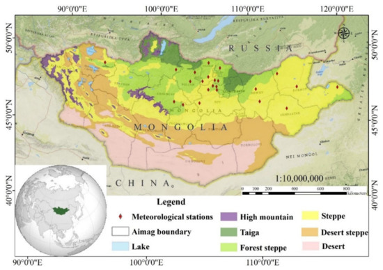
Figure 1.
Locations of soil moisture meteorological stations and six vegetation zones.
The Mongolian climate is highly continental, with arid and semi-arid conditions [33], and has four distinct seasons, high temperature fluctuations, and little precipitation. About 85% of the total precipitation falls from April to September, of which about 50–60% falls during July and August [34]. The mean annual temperature is −8 °C in the northern areas and 6 °C in southern regions [34]. The total soil moisture decreases, going from the north to the south of Mongolia [35] due to the different regions of Mongolian vegetation [36]. The annual precipitation is 300–400 mm in the taiga, high mountain, and forest steppe zones: 150–250 mm in the steppe, 100–150 mm in the desert steppe, and 50–100 mm in the desert (Gobi) region. Most of the cropland is located in the north of Mongolia, which encompasses the forest steppe and steppe zones.
2.2. Remote Sensing Data
2.2.1. SMAP
On 31 January 2015, NASA launched SMAP, which has an initial L-band with both radar and radiometer to assess soil moisture [37]. The daily coverage started on 31 March 2015 at a spatial resolution of 3–36 km. The average monthly SMAP data were obtained using daily SMAP with 9 km resolution. We downloaded daily SMAP L3 Radiometer Global Daily 9 km EASE-Grid Soil moisture data (SPL3SMP_E.003) through the Application for Extracting and Exploring Analysis Ready Samples (AppEEARS) between 2015 and 2020 [38]. AppEEARS is a useful tool for time series analysis in specific regions and at certain scales. It provides data by enabling users to download only the information (geospatial datasets using spatial, temporal, and band/layer parameters) needed from several federal archives (https://lpdaacsvc.cr.usgs.gov/appeears/). The downloaded images were preprocessed with the ENVI 5.3 and ArcGIS 10.3 software to obtain the monthly soil moisture data.
2.2.2. MODIS
We used MODIS products over a 10-year period (2010–2020) to observe the dynamic range of the NDVI and LST. Zhang et al. [39] used a similar approach to detect anomalies using MODIS land products via time series analysis. Accordingly, monthly composites of 1 km spatial resolution MOD13A3 [40] and MOD11A2 [41] data from MODIS and the National Aeronautics and Space Administration (NASA) Earth Observing system (https://lpdaac.usgs.gov/product_search/) data were used. The MODIS vegetation indices (MOD13A3) version 6 data are provided monthly at 1 km spatial resolution in the sinusoidal projection [40]. The MOD11A2 version 6 product provides an average eight-day-per-pixel Land Surface Temperature and Emissivity (LST&E) with a 1 km spatial resolution [41]. We calculated eight-day LST as monthly averages using product version 6 (MOD11A1). The Application for Extracting and Exploring Analysis Ready Samples (AppEEARS) tool offers vegetation and LST products of MODIS for long-term data [42].
2.3. CRU Data and Meteorological Data
CRU TS (Climatic Research Unit gridded Time Series) data are broadly used in climate studies and are available at 0.5 × 0.5 degrees over the whole surface of the Earth. It provides a monthly land-based gridded high-resolution dataset from 1901. The CRU dataset is derived by the interpolation of monthly weather station observations of extensive networks. The database is updated annually [43]. The CRU TS global data freely downloadable and accessible online (https://crudata.uea.ac.uk/cru/data/). We applied CRU TS v4 to this research for available temperature and precipitation data between 2010 and 2019.
The meteorological station data were provided by the Information and Research Institute of Meteorology, Hydrology and Environment (IRIMHE) of Mongolia website (http://tsag-agaar.gov.mn/). There were limited stations for soil moisture measurement in croplands over Mongolia. Soil moisture content was acquired at depths of 0–20 cm and 0–50 cm at monthly intervals (the 7th, 17th, and 27th days of each month) from April to September due to seasonal conditions [44]. Soil moisture content was averaged over the monthly intervals from May to August (2015–2020). The selected meteorological stations are shown in Figure 1, and the locations of the stations have been categorized into two vegetation zones (Table 1).

Table 1.
Location of the agricultural meteorological stations of soil moisture.
2.4. Crop Yield Statistical Data
Soil moisture is one of the most important factors in the agricultural sectors of Mongolia. The National Statistical Organization (NSO) website (http://nso.mn/) of Mongolia provides information on crop yields every year in the subprovinces. The NSO has been accumulating data on croplands and harvests collected from agricultural enterprises and local farmers through the statistical departments and offices of each province. Crop yield information was applied for the validation of soil moisture distribution in Mongolia from 2010 to 2019. The total harvest includes the amount of potatoes, fodder crops, cereals, fruits, vegetables, etc. (in thousands of tons), and the crop yield information is averaged every year. Crop yield is shown as the amount of agricultural production per unit area (from 1 hectare). The crop yield per hectare is estimated as the ratio of total harvest to total sown area [45].
3. Methodology
In this study, the structure of the spatial distribution of the soil moisture and time series analysis based on SMAP and MODIS products is given in the flowchart in Figure 2.
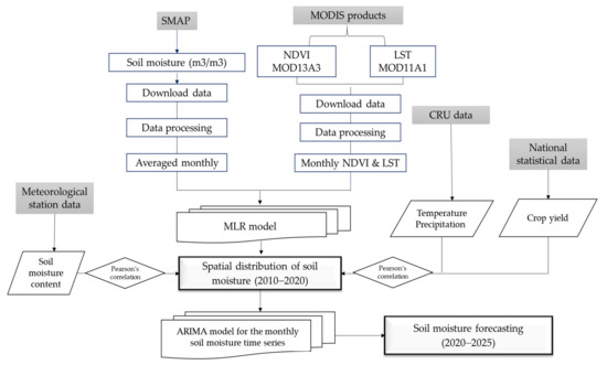
Figure 2.
Flowchart of the soil moisture distribution of Mongolia based on satellite images.
The first involved downloading the data and processing it, e.g., by the SMAP satellite, NDVI, and LST from the MODIS satellite. After data processing, a multiple linear regression model was developed. Prepared monthly soil moisture content from the station, temperature/precipitation of CRU data, and yearly crop yield information from the NSO were applied for validation of the estimated soil moisture over Mongolia. Finally, time series analysis and forecasting model were used for the prediction of estimated monthly soil moisture.
3.1. Multiple Linear Regression—SM-MOD
Multiple linear regression models have often been used in natural resource studies, and these involve calculating the dependent variable Y by applying a linear combination of independent variables Xi. The linear regression form is shown in the following equation [46]:
where β0, βm (m > 0) are constant terms corresponding to the connection, the regression coefficients, and the model error, Xm,i, respectively. The input variables (Xi) describe the output variable (Yi) according to the results of the multiple regression model. Therefore, each input variable has different information that means all input variables should not be collinear. We used p-value statistics to estimate the significance of each variable for input variable selection [46]. The variance inflation factor (VIF) is applied to detect collinearity (also called multicollinearity) among predictors in regression models [47,48]. The VIF values are between 1 and 10, which means that there is no multicollinearity for the regression model. After these analyses, a combination of p-value and VIF measures was used. Additionally, the independent variables are normally distributed for the assumptions of the linear regression model. Table 2 shows the statistical variables computed from satellite images.
Table 2.
Statistical variables of inputs, minimum (Min), maximum (Max), mean, and standard deviation (SD).
3.2. ARIMA Model
The Box‒Jenkins time series models are named after the statisticians George Box and Gwilym Jenkins [49]. These models generate forecast values based on the statistical parameters of observed time series data and are used in many fields. The Box‒Jenkins Autoregressive Integrated Moving Average (ARIMA) model is a combination of the Autoregressive (AR), Integrated (I), and Moving Average (MA) terms. The Box‒Jenkins model describes a wide class of models forecasting univariate time series that can be made stationary by applying transformations such as differencing of nonstationary series one or more times to achieve stationarity [50,51].
A seasonal ARIMA model is denoted by ARIMA (p, d, q), where p is the number of autoregressive terms, q is the number of moving average terms, and d represents the number of differences applied to the series [52].
The AR (p) model is defined as
where φ1, φ2, …, φn are the autoregressive coefficients, c is a constant, and ut is white noise. In the autoregressive model of order p, the value of the time series at t, Xt depends upon its previous p-values and a random disturbance (the stochastic part).
The MA (p) model is defined as
where θ1, θ2, …, θq are the moving average coefficients and {zt} is a white noise process with mean 0 and variance σ2. Combing autoregressive and moving average models, we get Equation (4):
where xt denotes the dth difference of Xt.
This defines the autoregressive moving average (ARIMA) process of p and q order and difference d, or ARIMA (p, q) [26].
There are many methods and criteria for selecting the order of an AR, MA, or ARIMA model. One of them is based on the so-called information criteria and computes the values of Akaike’s information criterion (AIC) and the Bayesian information criterion (BIC) or Schwarz criterion, with smaller values of AIC and BIC preferred [53,54]. The most commonly used approach for checking the model’s adequacy is to examine the residuals by using the autocorrelation function (ACF) and partial autocorrelation function (PACF) graphs. If the selected model is appropriate, the residual graphs of both correlation functions should be white noise, indicating no remaining correlation.
3.3. Model Validation
The model was implemented to evaluate the next step. Pearson’s correlation (r) [55] values were applied for the comparison for estimated soil moisture and observed soil moisture and crop yield values. The coefficients of the Pearson’s correlation (r) are given in Equation (5):
where Xi and Yi are the individual derivations and measurements of variables X and Y, respectively. and are the means of X and Y, respectively. The correlation coefficient (r) ranges between −1 and 1. If r is equal to zero, this means that there is no linear association between the variables. If r is equal to 1, there is a perfect positive linear relationship between the variables, and all individuals sampled would be exactly on the same straight line with a positive slope. If 0 < r < 1, this means a positive linear trend, but sampled individuals would be scattered around this common trend line; the smaller the absolute r value, the less well the data can be characterized by a single linear relationship. If r is positive and r values are close to 1, this describes a valuable relationship between variables [56]. Linear Pearson’s correlation (r) was determined at a monthly timescale [44,55] for the satellite-derived and meteorological station/NSO data.
4. Results
4.1. SM-MOD—Multiple Linear Regression Model
The linear regression model in Equation (1) was applied to estimate soil moisture in Mongolia, with 1 km resolution. The multicollinearity tests for all variables (NDVI and LST) were determined as in Table 3. The VIF values were lower than five, which shows that there was no multicollinearity for the regression model. Also, histogram normality test has been checked by the Jarque-Bera test for the linear regression model. In this test, if the probability of Jarque-Bera greater than 0.05% or 5%, then we accepted the null hypothesis, which means that the residuals were normally distributed. Table 3 summarizes the multiple linear regression model coefficients, p-values, standard error, t-statistics, VIF statistics. The monthly NDVI and LST explained 78% of the variation in soil moisture. The F-statistic was less than 0.05, which means that this model can be used for soil moisture analysis.
Table 3.
Result of the linear regression model.
In this research, we assume that SM is derived from the satellite and depends on the independent variables NDVI and LST, while SMAP is the dependent variable. From the assumption, a multiple regression model has been developed. Finally, the MLR model resulted in Equation (6):
where SMMOD is the modeled soil moisture; constant coefficients were estimated from Table 3. Figure 3 shows graphs of the actual, fitted, and residual values of the linear regression. The figure suggests that in most of the studied months, the correlation between the real-life situation and the model was high.
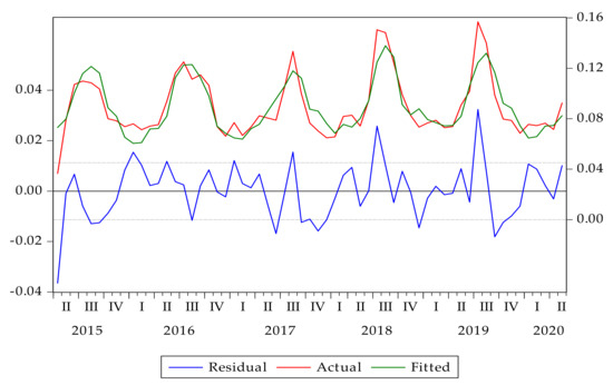
Figure 3.
Actual, fitted, and residual values of the multiple regression model.
Soil moisture (SM-MOD) was calculated using Equation (6), with values in m3/m3. The lowest value of 0 indicates dry areas and the highest value of 0.35 m3/m3 indicates wet areas. Figure 4 represents the spatial distribution of monthly soil moisture over Mongolia. Monthly SM maps were averaged by month between 2010 and 2020. During the years 2010–2020, the winter had the lowest soil moisture (November, December, and January), and spring also had low soil moisture (February, March, and April). The summer showed high soil moisture in May, June, and July. However, the autumn showed the highest soil moisture in August, September, and October (Figure 4). Apparently, increased soil moisture is observed in the northern part, which is taiga, forest steppe, and steppe zones, while low soil moisture is restricted to the southern part of Mongolia, which is mostly desert steppe and desert vegetation.
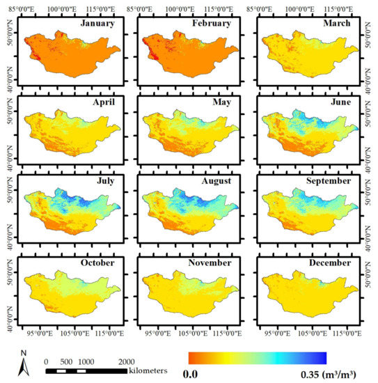
Figure 4.
Spatial distribution of soil moisture content from the model (SMMOD) (averaged monthly from 2010 to 2020).
4.2. Comparison between MLR Model and SMC from the Meteorological Station
In general, the estimation of soil moisture from the model was reasonably accurate, as confirmed by applying satellite images. Figure 5a–d describe the correlation between SMAP and SM-MOD with the SMC from the meteorological station at 0–20 and 0–50 cm depths. Table 4 shows the correlations of the SMAP and SM-MOD with the SMC from the meteorological stations at different depths. The correlation coefficients (r) between SMAP and SMC from meteorological stations were 0.279 (Figure 5a) and 0.181 (Figure 5b) at 0–20 and 0–50 cm depths, respectively. This was statistically significant, with root mean square error (RMSE) values of 0.094 m3/m3 and 0.098 m3/m3, as shown in Table 4a. Table 4b indicates that the values of correlation coefficients (r) were 0.191 between SM-MOD and SMC at 0–20 cm depth from the meteorological station, which was statistically significant, with an RMSE of 0.090 m3/m3 (p < 0.0001; Figure 5c), and 0.126 between SM-MOD and SMC at 0–50 cm depth from the meteorological station, which was also statistically significant, with an RMSE of 0.091 m3/m3 (p < 0.005; Figure 5d). The confidence intervals of 95% were between SM-MOD and SMC at 0–20 cm depth from the meteorological station from 0.104 to 0.276, and with SMC at 0–50 cm from the meteorological station from 0.038 to 0.213.
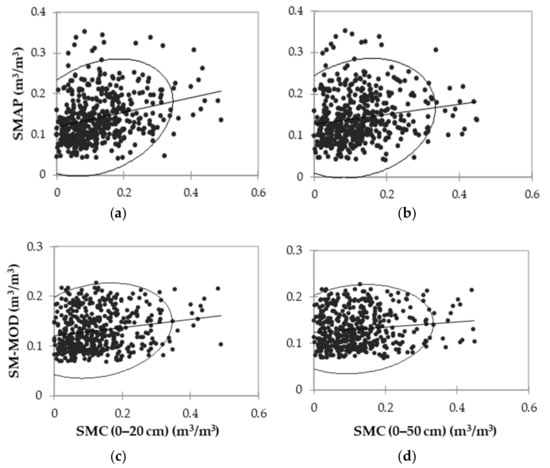
Figure 5.
Scatter diagram of SMAP and SM-MOD with SM measurements from the meteorological stations for different depths from May to August of 2015–2020 over the study area: (a) SMAP and SMC from the meteorological stations at 0–20 cm depth; (b) SMAP and SMC from the meteorological stations at 0–50 cm depth; (c) SM-MOD and SMC from the meteorological stations at 0–20 cm depth; (d) SM-MOD and SMC from the meteorological stations at 0–50 cm depth.
Table 4.
Correlation between (a) SMAP and (b) SM-MOD with the SMC from the meteorological stations at the different depths from May to August of 2015–2020.
4.3. Comparison between SM-MOD and CRU Data
We also examined the trends of monthly precipitation and temperature from the CRU data. Figure 6 displays the time series of monthly precipitation, temperature, and SM-MOD from 2010 to 2020 in Mongolia. The highest precipitation was observed in July 2018, and the highest SM-MOD value was in August 2018. From the comparison, when the precipitation was high, then the following month’s soil moisture was high, which means that in Mongolia, the soil moisture directly depends on precipitation.
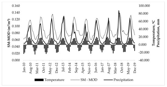
Figure 6.
Comparison between monthly precipitation (mm), temperature (°C), and SM-MOD (m3/m3) from January 2010 to December 2019 in Mongolia.
Figure 7a–c describes the correlation between SM-MOD and the temperature and precipitation. Table 5 shows the correlations of the SM-MOD with the temperature and precipitation from the CRU data over Mongolia. It indicates that the values of correlation coefficients (r) were 0.802 between SM-MOD and temperature, which was statistically significant (p < 0.0001; Figure 7b), and 0.826 between SM-MOD and precipitation, which was also statistically significant (p < 0.0001; Figure 7c). The confidence intervals of 95% were between SM-MOD from the model and monthly temperature from 0.728 to 0.858, and with monthly precipitation from 0.759 to 0.876 over Mongolia.
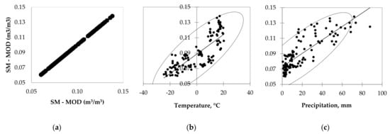
Figure 7.
Scatter diagram of the monthly SM-MOD (m3/m3), monthly temperature (°C), and monthly precipitation (mm) from 2010 to 2020 over the study area: (a) SM-MOD and SM-MOD; (b) SM-MOD and temperature (°C); (c) SM-MOD and precipitation (mm).
Table 5.
Correlation among the monthly SM-MOD with the monthly temperature (°C) and monthly precipitation (mm) from the CRU data between 2010 and 2020.
4.4. Comparison between SM-MOD and Crop Yield
We considered the crop yield information for every year to correlate with SM-MOD from the model. The National Statistical Organization (NSO) provides every province’s crop yield information since 2010. Figure 8 shows the trends of averaged SM-MOD from May to September of 2010–2019 and the observed total crop yield data for each year (2010–2019).
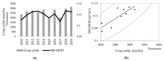
Figure 8.
Comparison of the SM-MOD and crop yield information: (a) yearly crop yield (ton/ha) and averaged SM-MOD from May to September (2010–2019); (b) scatter diagram of SM-MOD and crop yield information.
To apply the model to the use, we examined the relationship between SM-MOD and crop yield over Mongolia. The results show that there is a significant trend in the SM-MOD. It was statistically significantly (p < 0.003) correlated with the crop yield, with r = 0.835 (Table 6).
Table 6.
Correlation between the averaged SM-MOD from May to September for 2010–2019 and the yearly crop yield from NSO for 2010–2019.
4.5. ARIMA Model of Soil Moisture
We selected the most appropriate model for the time series from the possible models. We selected our model using these criteria: first, the most significant coefficients; second, the lowest volatility; third, the highest adjusted R-squared; and last, the lowest Akaike’s information criterion (AIC)/Schwarz information criterion (SIC). Since the theory behind ARMA estimation is based on a stationary time series, we first used the transformation based on a logarithm and considered the first difference of the soil moisture time series. According to the unit root test, the differenced series is a stationary series, so we applied the plots of ACF and PACF to identify the structure of the model. The plots and statistical tests showed that the ARIMA (12, 1, 12) model was suitable for the log time series of soil moisture. The estimation results and the actual, fitted residual graphs of the model are shown in Table 7 and Figure 9, respectively. The residual diagnostics tests suggest that the estimation residuals are white noise. The final results indicate the good performance of the model, and we can say that about 82% of the variability in the soil moisture was predicted by the selected model (Table 7).
Table 7.
Results of the time series analysis for soil moisture.
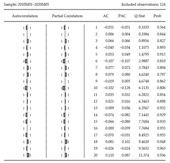
Figure 9.
Correlogram of residuals squared of the autocorrelation function (ACF) and partial autocorrelation function (PACF).
The selected model is written as follows:
or, equivalently, as
where is the log values of soil moisture at time and is the error term at time .
The above model shows that the soil moisture at time depends on the value of soil moisture of previous months and also on the error terms of 12 months ago.
Partial autocorrelation (PAC) measures the correlation between observations that are p periods apart after controlling for correlations at intermediate lags (i.e., lags less than p). The correlogram of the residuals is flat, which indicates that all information has been captured (Figure 9). A flat correlogram of the residuals is ideal. Therefore, the forecast will be based on this model.
One of the main purposes of the ARMA and ARIMA models is to provide short-term forecasts. Hence, we have predicted the values of soil moisture from 2020 to 2025 using the selected model. Figure 10 shows the forecasting results for soil moisture from 2020 to 2025 with a 95% confidence interval, which is the range within which the actual dependent value should fall a given percentage of the time (the level of confidence). For forecasting, the root mean squared error was 0.002, and the bias proportion was 0.044. Figure 11 compares the actual soil moisture and soil moisture forecasting (in m3/m3) from January to May 2020. The prediction from February and April is almost the same as the actual soil moisture and there were slight deviations when predicting March and May. Overall, the model demonstrated accurate forecasting of soil moisture.
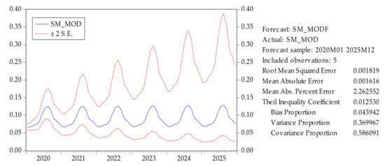
Figure 10.
Soil moisture forecasting from the ARIMA model (m3/m3).
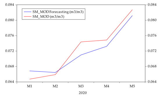
Figure 11.
Comparison graph of the real soil moisture and soil moisture forecasting.
The essence of an appropriate ARIMA model is to forecast the future trends of series. Hence, we used the past information of the soil moisture series itself. The forecast was based on the final selected model, ARIMA (12, 1, 12).
The forecasting values of soil moisture are given in Figure 12, with the kernel density of the values on the y axis.
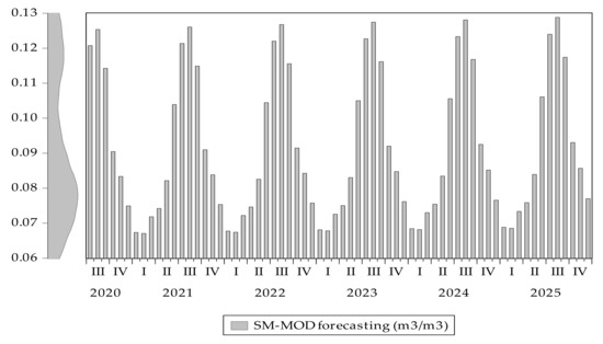
Figure 12.
Predicting soil moisture trend until December 2025.
5. Discussion
In the present study, we used a linear regression model to estimte the spatial distribution of soil moisture over Mongolia by considering satellite images (SMAP and MODIS). We estimated the monthly (January–December) soil moisture during the period 2010–2020 in Mongolia. The SM model performance was validated by comparison with SMC from the agricultural meteorological stations, with data on precipitation, temperature, crop yield, etc. The correlation has shown that the model (SM-MOD) gives accurate information on the soil moisture for each month. Moreover, the present model has the advantage of recognizing soil moisture spatial distribution with a high spatial resolution (1 km); this is the first time such information has been gathered for Mongolia. Therefore, we established the ARIMA model for soil moisture forecasting based on estimated soil moisture between 2010 and 2020. The results provide the monthly spatial distribution of soil moisture, which is valuable data for use in numerous contexts, including agricultural management, drought monitoring, assessment of climate change, flooding, determining pasture and land degradation. Land degradation in central Mongolia is mostly caused by overgrazing; however, changes in summertime precipitation have also occurred [57]. Mongolian grassland is decreasing, and drought is increasing [58]. Our research on time series analysis for monthly SM-MOD forecasting is vital for the monitoring of land degradation and drought.
The results of correlation coefficients are low because of limited data availability at the agricultural meteorological station. However, the correlation was statistically significant at p < 0.0001 (0–20 cm) and p < 0.005 (0–50 cm), respectively, between SM-MOD and SMC from the meteorological stations at different depths. From Figure 6, we see that the previous month’s precipitation directly impacted the soil moisture during the growing season (June–September). The correlation between SM-MOD and temperature had correlation coefficients (r) of 0.80 (statistically significant at p < 0.0001) and 0.83 (statistically significant at p < 0.0001). However, SM-MOD compared with the crop yield for each year (2010–2019) had a correlation coefficient (r) of 0.84.
Therefore, the time series analysis for monthly soil moisture forecasting was developed over Mongolia based on the established ARIMA model. From the study, we selected the ARIMA (12, 1, 12) model, which was most suitable for the SM-MOD time series, for prediction, in which the values of soil moisture (SM-MOD) were predicted from 2020 to 2025 using the selected model. Forecasting results are shown with a 95% confidence interval. Time series SM-MOD data will provide valuable information for decision-makers and researchers. SM-MOD time series and forecasting data are good sources of data for long-term agricultural management, planning, and climate change and drought monitoring.
In terms of applications, this multiple linear regression model is a practical tool for the reliable and timely monitoring of droughts; thus, the advantage of this research lies in providing valuable information for decision-makers and farmers. In further studies, we will investigate seasonal soil moisture in different vegetation zones using this method along with field measurements.
6. Conclusions
Soil moisture is an important factor for the agricultural land in Mongolia. The model used in this paper is suitable for use in agricultural areas and has useful applications for agricultural management (irrigation, pasture, and hayfield yield) and drought monitoring in Mongolia. Time series analysis is one of the main tools for analyzing and predicting future trends of soil moisture. Most previous studies have examined soil moisture by comparing it with climate factors that were analyzed based on correlation analysis and multilinear regression [7,59,60]. The LST/NDVI combination method may prove to be a robust method for estimating SM; this combination is easy to operate and has a strong physical basis [7].
In general, the model’s performance in determining soil moisture was practically assessed using satellite images. This study took Mongolia as the study area, divided into six vegetation zones. The linear regression method was applied in soil moisture estimation using SMAP and MODIS satellite images. From the model, the spatial distribution of soil moisture was developed monthly from 2010 to 2020. The soil moisture was high in the north, while low soil moisture was observed in southern Mongolia, especially during the warm season. Then output maps were compared with the soil moisture content from the agricultural meteorological stations and precipitation/temperature from the CRU data. The results show that the estimated soil moisture was statistically significantly correlated with the actual soil moisture content reported by the station. Moreover, the estimated soil moisture (SM-MOD), when compared with the crop yield, showed a high correlation, though there is a need for more accurate, detailed ground-measured data. Finally, we performed a time series analysis of soil moisture from 2010 to 2020 and predicted soil moisture until 2025 in this study area. Overall, the developed SM model and time series method can both be used to investigate the changes in soil moisture in Mongolia, so it is reasonable to use them in agriculture, hydrology, and climate science. However, this linear regression model should be elaborated to suit each vegetation zone or eco-climate regions in the applied study area.
Author Contributions
E.N. analyzed all data with ArcGIS 10.3 & ENVI 4.7 and computed the statistical analysis with E-view 9.0 and XLSTAT2020 software. Also, E.N. wrote the first draft. T.R. and P.D.M. provided useful advice and revised the manuscript. B.D. helped the statistical analysis and time series methods. All authors contributed to the final manuscript. All authors have read and agreed to the published version of the manuscript.
Funding
This research received no external funding.
Institutional Review Board Statement
Not applicable.
Informed Consent Statement
Not applicable.
Acknowledgments
The first author is very grateful to the European Union ERASMUS-IMPAKT-2016 program scholarship, allowing her to pursue her study at the Ghent University, Belgium. Also, very thankful to the Department of Geography for research supports and very thankful to the co-authors, besides special thanks to Frieke Vancoillie of the Ghent University given the specific comments. We are grateful to the Information and Research Institute and Research Institute of Meteorology, Hydrology and Environment (IRIMHE) and National Statistical Office (NSO) of Mongolia for providing us soil moisture measurements and crop yield growth data used in this research. We acknowledge the anonymous reviewers for their valuable comments, which remarkably improved our paper.
Conflicts of Interest
The authors declare no conflict of interest.
References
- Gao, X.; Wu, P.; Zhao, X.; Wang, J.; Shi, Y. Effects of land use on soil moisture variations in a semi-arid catchment: Implications for land and agricultural water management. Land Degrad. Dev. 2014, 25, 163–172. [Google Scholar] [CrossRef]
- Deryng, D.; Sacks, W.J.; Barford, C.C.; Ramankutty, N. Simulating the effects of climate and agricultural management practices on global crop yield. Glob. Biogeochem. Cycles 2011, 25. [Google Scholar] [CrossRef]
- Wang, X.; Wang, B.; Xu, X.; Liu, T.; Duan, Y.; Zhao, Y. Spatial and temporal variations in surface soil moisture and vegetation cover in the Loess Plateau from 2000 to 2015. Ecol. Indic. 2018, 95, 320–330. [Google Scholar] [CrossRef]
- Park, S.; Im, J.; Park, S.; Rhee, J. Drought monitoring using high resolution soil moisture through multi-sensor satellite data fusion over the Korean peninsula. Agric. Forest Meteorol. 2017, 237, 257–269. [Google Scholar] [CrossRef]
- Natsagdorj, E.; Tsolmon, R.; Martin, K.; Batchuluun, T.; Chimgee, D.; Oyunbileg., T.; Ulam-Orgikh, D. An integrated methodology for soil moisture analysis using multispectral data in Mongolia. Geo-Spat. Inf. Sci. 2017, 20, 46–55. [Google Scholar] [CrossRef][Green Version]
- Rahimzadeh-Bajgiran, P.; Berg, A. Soil moisture retrievals using optical/TIR methods. In Satellite Soil Moisture Retrieval: Techniques and Applications; Elsevier Inc.: Amsterdam, The Netherlands, 2016; pp. 47–72. [Google Scholar]
- Zhang, D.; Zhou, G. Estimation of Soil Moisture from Optical and Thermal Remote Sensing: A Review. Sensors 2016, 16, 1308. [Google Scholar] [CrossRef] [PubMed]
- Peng, J.; Loew, A. Recent Advances in Soil Moisture Estimation from Remote Sensing. Water 2017, 9, 530. [Google Scholar] [CrossRef]
- Jung, C.; Lee, Y.; Cho, Y.; Kim, S. A Study of Spatial Soil Moisture Estimation Using a Multiple Linear Regression Model and MODIS Land Surface Temperature Data Corrected by Conditional Merging. Remote Sens. 2017, 9, 870. [Google Scholar] [CrossRef]
- Vani, V.; Pavan Kumar, K.; Ravibabu, M.V. Temperature and vegetation indices based surface soil moisture estimation: A remote sensing data approach. In Springer Series in Geomechanics and Geoengineering; Springer: Berlin/Heidelberg, Germany, 2019; pp. 281–289. [Google Scholar]
- Hong, Z.; Zhang, W.; Yu, C.; Zhang, D.; Li, L.; Meng, L. SWCTI: Surface Water Content Temperature Index for Assessment of Surface Soil Moisture Status. Sensors 2018, 18, 2875. [Google Scholar] [CrossRef]
- Brocca, L.; Crow, W.T.; Ciabatta, L.; Massari, C.; Rosnay, P.D.; Enenkel, M.; Hahn, S.; Amarnath, G.; Camici, S.; Tarpanelli, A.; et al. A Review of the Applications of ASCAT Soil Moisture Products. IEEE J. Sel. Top. Appl. Earth Obs. Remote Sens. 2017, 10, 2285–2306. [Google Scholar] [CrossRef]
- Chan, S.K.; Bindlish, R.; Njoku, E.; Jackson, T.; Colliander, A.; Chen, F.; Burgin, M.; Dunbar, S.; Piepmeier, J.; Yueh, S.; et al. Assessment of the SMAP Passive Soil Moisture Product. IEEE Trans. Geosci. Remote Sens. 2016, 54, 4994–5007. [Google Scholar] [CrossRef]
- Zhang, X.; Zhang, T.; Zhou, P.; Shao, Y.; Gao, S. Validation Analysis of SMAP and AMSR2 Soil Moisture Products over the United States Using Ground-Based Measurements. Remote Sens. 2017, 9, 104. [Google Scholar] [CrossRef]
- Chen, F.; Crow, W.T.; Colliander, A.; Cosh, M.H.; Jackson, T.J.; Bindlish, R.; Reichle, R.H.; Chan, S.K.; Bosch, D.D.; Starks, P.J.; et al. Application of Triple Collocation in Ground-Based Validation of Soil Moisture Active/Passive (SMAP) Level 2 Data Products. IEEE J. Sel. Top. Appl. Earth Obs. Remote Sens. 2017, 10, 489–502. [Google Scholar] [CrossRef]
- Zeng, J.; Chen, K.S.; Bi, H.; Chen, Q. A Preliminary Evaluation of the SMAP Radiometer Soil Moisture Product over United States and Europe Using Ground-Based Measurements. IEEE Trans. Geosci. Remote Sens. 2016, 54, 4929–4940. [Google Scholar] [CrossRef]
- Nemani, R.; Running, S. Land cover characterization using multitemporal Red, Near-Ir, and Thermal-Ir data from NOAA/AVHRR. Ecol. Appl. 1997, 7, 79–90. [Google Scholar] [CrossRef]
- Lambin, E.F.; Ehrlich, D. The surface temperature-vegetation index space for land cover and land-cover change analysis. Int. J. Remote Sens. 1996, 17, 463–487. [Google Scholar] [CrossRef]
- Chae, S.-H.; Park, S.-H.; Lee, M.-J. A Study on the Observation of Soil Moisture Conditions and its Applied Possibility in Agriculture Using Land Surface Temperature and NDVI from Landsat-8 OLI/TIRS Satellite Image. Korean J. Remote Sens. 2017, 33, 931–946. [Google Scholar] [CrossRef]
- Saha, A.; Patil, M.; Goyal, V.C.; Rathore, D.S. Assessment and Impact of Soil Moisture Index in Agricultural Drought Estimation Using Remote Sensing and GIS Techniques. Proceedings 2018, 7, 2. [Google Scholar] [CrossRef]
- Dandridge, C.; Fang, B.; Lakshmi, V. Downscaling of SMAP Soil Moisture in the Lower Mekong River Basin. Water 2019, 12, 56. [Google Scholar] [CrossRef]
- Leary, N. Climate Change and Vulnerability and Adaptation: Two Volume Set; Routledge: Abingdon, UK, 2008. [Google Scholar]
- Yatagai, A.; Yasunari, T. Interannual Variations of Summer Precipitation in the Arid/semi-arid Regions in China and Mongolia: Their Regionality and Relation to the Asian Summer Monsoon. J. Meteorol. Soc. Jpn. Ser. II 1995, 73, 909–923. [Google Scholar] [CrossRef]
- Nandintsetseg, B.; Shinoda, M. Seasonal change of soil moisture in Mongolia: Its climatology and modelling. Int. J. Clim. 2011, 31, 1143–1152. [Google Scholar] [CrossRef]
- Shinoda, M.; Nandintsetseg, B. Soil moisture and vegetation memories in a cold, arid climate. Glob. Planet. Chang. 2011, 79, 110–117. [Google Scholar] [CrossRef]
- Box, G.E.P.; Jenkins, G.M.; Reinsel, G.C. Time Series Analysis Forecasting and Gontrol; John Willey & Sons Inc.: Hoboken, NJ, USA, 2016. [Google Scholar]
- Singh, S.; Kaur, S.; Kumar, P. Forecasting Soil Moisture Based on Evaluation of Time Series Analysis. Lect. Notes Electr. Eng. 2020, 609, 145–156. [Google Scholar] [CrossRef]
- Tian, M.; Wang, P.; Khan, J. Drought Forecasting with Vegetation Temperature Condition Index Using ARIMA Models in the Guanzhong Plain. Remote Sens. 2016, 8, 690. [Google Scholar] [CrossRef]
- Karthika, M.; Thirunavukkarasu, V. Forecasting of meteorological drought using ARIMA model. Indian J. Agric. Res. 2017, 51, 103–111. [Google Scholar] [CrossRef]
- Han, P.; Wang, P.X.; Zhang, S.Y.; Zhu, D.H. Drought forecasting based on the remote sensing data using ARIMA models. Math. Comput. Model. 2010, 51, 1398–1403. [Google Scholar] [CrossRef]
- Mishra, A.K.; Desai, V.R. Drought forecasting using stochastic models. Stoch. Environ. Res. Risk Assess. 2005, 19, 326–339. [Google Scholar] [CrossRef]
- Otgonbayar, M.; Atzberger, C.; Chambers, J.; Amarsaikhan, D.; Böck, S.; Tsogtbayar, J. Land Suitability Evaluation for Agricultural Cropland in Mongolia Using the Spatial MCDM Method and AHP Based GIS. J. Geosci. Environ. Prot. 2017, 5, 238–263. [Google Scholar] [CrossRef]
- Nandintsetseg, B.; Greene, J.S.; Goulden, C.E. Trends in extreme daily precipitation and temperature near lake Hövsgöl, Mongolia. Int. J. Clim. 2007, 27, 341–347. [Google Scholar] [CrossRef]
- Batima, P.; Natsagdorj, L.; Gombluudev, P.; Erdenetsetseg, B. Observed climate change in Mongolia. Assess. Imp. Adapt. Clim. Chang. Work Pap. 2005, 12, 1–26. [Google Scholar]
- Natsagdorj, E.; Renchin, T. Determination of moisture in Mongolia using remotely sensned data. In Proceedings of the Asian Conference on Remote Sensing, Hanoi, Vietnam, 1–5 November 2010; p. 921. [Google Scholar]
- Yunatov, A.A. Vegetation Map of the Mongolian Peoples’ Republic 1:1,500,000. Akad. Nauk SSSR Ai MNP 1979. [Google Scholar]
- Entekhabi, D.; Njoku, E.G.; O’Neil, P.E.; Kellogg, K.H.; Crow, W.T.; Edelstein, W.N.; Entin, J.K.; Goodman, S.D.; Jackson, T.J.; Johnson, J.; et al. The soil moisture active passive (SMAP) mission. Proc. IEEE 2010, 98, 704–716. [Google Scholar] [CrossRef]
- O’Neill, J.C.; Chan, S.; Njoku, E.G.; Jackson, T.; Bindlish, R.; NASA National Snow and Ice Data Center Distributed Active Archive Center. SMAP Enhanced L3 Radiometer Global Daily 9 km EASE-Grid Soil Moisture, Version 3. 2019. Available online: https://nsidc.org/data/SPL3SMP_E/versions/3 (accessed on 7 September 2020).
- Zhang, J.; Roy, D.; Devadiga, S.; Zheng, M. Anomaly detection in MODIS land products via time series analysis. Geo-Spat. Inf. Sci. 2007, 10, 44–50. [Google Scholar] [CrossRef]
- Didan, K.; NASA EOSDIS Land Processes DAAC. MOD13A3 MODIS/Terra Vegetation Indices Monthly L3 Global 1 km SIN Grid V006. 2015. Available online: https://lpdaac.usgs.gov/products/mod13a3v006/ (accessed on 8 June 2020).
- Hulley, G.; Wan, Z.; Hook, S.; NASA EOSDIS Land Processes DAAC. MOD11A2 MODIS/Terra Land Surface Temperature/Emissivity 8-Day L3 Global 1km SIN Grid V006. 2015. Available online: https://lpdaac.usgs.gov/products/mod11a2v006/ (accessed on 30 May 2020).
- AppEEARS Team; NASA EOSDIS Land Processes Distributed Active Archive Center (LP DAAC); USGS/Earth Resources Observation and Science (EROS) Center. Application for Extracting and Exploring Analysis Ready Samples (AppEEARS). 2020. Available online: https://lpdaacsvc.cr.usgs.gov/appeears/ (accessed on 1 June 2020).
- Harris, I.; Osborn, T.J.; Jones, P.; Lister, D. Version 4 of the CRU TS monthly high-resolution gridded multivariate climate dataset. Sci. Data 2020, 7, 1–18. [Google Scholar] [CrossRef]
- Natsagdorj, E.; Renchin, T.; de Maeyer, P.; Dari, C.; Tseveen, B. Long-term soil moisture content estimation using satellite and climate data in agricultural area of Mongolia. Geocarto Int. 2019, 34, 722–734. [Google Scholar] [CrossRef]
- NSO. Agriculture. 2020. Available online: http://www.1212.mn/Stat.aspx?LIST_ID=976_L10_2&type=tables (accessed on 7 September 2020).
- Weisberg, S. Applied Linear Regression; John Wiley & Sons, Inc.: Hoboken, NJ, USA, 2005. [Google Scholar]
- Murray, L.; Nguyen, H.; Lee, Y.F.; Remmenga, M.D.; Smith, D.W. Models with variance inflation factors in regression models with dummy variables. In Proceedings of the Conference on Applied Statistics in Agriculture Kansas State University, Manhattan, KS, USA, 29–30 April 2012; pp. 161–177. [Google Scholar] [CrossRef]
- Harrell, F.E. Multivariable modeling strategies. In Regression Modeling Strategies; Springer: Cham, Switzerland, 2001; pp. 53–85. [Google Scholar]
- Box, G.E.P.; Jenkins, G.M. Time Series Analysis: Forecasting and Control.; Holden-Day: San Francisco, CA, USA, 1970. [Google Scholar]
- Box, G.E.P.; Pierce, D.A. Distribution of residual autocorrelations in autoregressive-integrated moving average time series models. J. Am. Stat. Assoc. 1970, 65, 1509–1526. [Google Scholar] [CrossRef]
- Box, G.E.P.; Jenkins, G.M.; MacGregor, J.F. Some Recent Advances in Forecasting and Control. Appl. Stat. 1974, 23, 158. [Google Scholar] [CrossRef]
- Rahman, A.; Hasan, M.M. Modeling and Forecasting of Carbon Dioxide Emissions in Bangladesh Using Autoregressive Integrated Moving Average (ARIMA) Models. Open J. Stat. 2017, 7, 560–566. [Google Scholar] [CrossRef]
- Adnan, R.M.; Yuan, X.; Kisi, O.; Curtef, V. Application of Time Series Models for Streamflow Forecasting. Civ. Environ. Res. 2017, 9, 56–63. [Google Scholar]
- Hyndman, R.J.; Koehler, A.B. Another look at measures of forecast accuracy. Int. J. Forecast. 2006, 22, 679–688. [Google Scholar] [CrossRef]
- Sedgwick, P. Pearson’s correlation coefficient. BMJ 2012, 345, e4483. [Google Scholar] [CrossRef]
- Puth, M.T.; Neuhäuser, M.; Ruxton, G.D. Effective use of Pearson’s product-moment correlation coefficient. Anim. Behav. 2014, 93, 183–189. [Google Scholar] [CrossRef]
- Hilker, T.; Natsagdorj, E.; Waring, R.H.; Lyapustin, A.; Wang, Y. Satellite observed widespread decline in Mongolian grasslands largely due to overgrazing. Glob. Chang. Biol. 2014, 20, 418–428. [Google Scholar] [CrossRef] [PubMed]
- Sternberg, T. Investigating the presumed causal links between drought and dzud in Mongolia. Nat. Hazards 2018, 92, 27–43. [Google Scholar] [CrossRef]
- Xia, L.; Song, X.; Leng, P.; Wang, Y.; Hao, Y.; Wang, Y. A comparison of two methods for estimating surface soil moisture based on the triangle model using optical/thermal infrared remote sensing over the source area of the Yellow River. Int. J. Remote Sens. 2019, 40, 2120–2137. [Google Scholar] [CrossRef]
- Wang, Y.; Yang, J.; Chen, Y.; Wang, A.; de Maeyer, P. The Spatiotemporal Response of Soil Moisture to Precipitation and Temperature Changes in an Arid Region, China. Remote Sens. 2018, 10, 468. [Google Scholar] [CrossRef]


Publisher’s Note: MDPI stays neutral with regard to jurisdictional claims in published maps and institutional affiliations. |
© 2021 by the authors. Licensee MDPI, Basel, Switzerland. This article is an open access article distributed under the terms and conditions of the Creative Commons Attribution (CC BY) license (http://creativecommons.org/licenses/by/4.0/).